Model for erosion-deposition patterns

Abstract

We investigate through computational simulations with a pore network model the formation of patterns caused by erosion-deposition mechanisms. In this model, the geometry of the pore space changes dynamically as a consequence of the coupling between the fluid flow and the movement of particles due to local drag forces. Our results for this irreversible process show that the model is capable to reproduce typical natural patterns caused by well known erosion processes. Moreover, we observe that, within a certain range of porosity values, the grains form clusters that are tilted with respect to the horizontal with a characteristic angle. We compare our results to recent experiments for granular material in flowing water and show that they present a satisfactory agreement.

I Introduction

Nature preservation and environmental protection are important issues on the agendas of governments and non-governmental organizations. Consequently, these issues have been the subject of intense study, where the main concern is to understand how the actions of human beings affect the environment. For example, deforestation and pollutant emissions are related to climate changes resulting in floods and erosion. In particular, erosion can be responsible for diminishing the quality of life, because it affects the soil causing a negative impact on the economy. Aside from its economical and ecological aspects, the erosion problem also attracts the interest of geologists and physicists. In geology, this is an extremely rich area as many of the patterns observed in nature stem from erosion or deposition processes. In physics, the formation of such patterns span a huge range of spatial and temporal scales. This pattern formation process is directly related to the transport of solid granular particles via a fluid and presents a rich phenomenology along with a variety of applications Behringer et al. (1999); Jaeger et al. (1996). Particular applications are fractal river basins, meandering rivers, dune fields, granular avalanches, and ripple marks on sand banks or on coastal continental platforms.

It is notoriously difficult to provide a fully consistent description of particle laden flows either from a one-phase or a two-phase point of view. Most of the practical knowledge of erosion comes from empirical laws often derived from field measurements. This has provoked interest in theoretical descriptions of these systems Kroy et al. (2002); Herrmann (1999); Ertas and Halsey (2002) and visualization of them in computational simulations. Several attempts to understand the dynamics of river basin formation from the statistical physics point of view have been made recently, but many questions are raised when one tries to relate basic transport properties to large-scale pattern forming instabilities Seybold et al. (2007). A fundamental open question is the following: how do objects made of granular materials respond to the action of external factors? Many experiments Daerr et al. (2003); Pouliquen (1999); Aranson et al. (2006); Pouliquen and Vallance (1999); Borzsonyi et al. (2005); Forterre and Pouliquen (2003); Pouliquen (2004); Midi (2004) have been performed in the last few years to answer this question. For example, in Fig. 1, we see a laboratory-scale experiment which reproduces a rich variety of natural patterns with few control parameters Daerr et al. (2003). These patterns are characterized by chevron alignments, what means that the paths created by the fluid present a characteristic angle that depends on the parameters varied in the experiment.

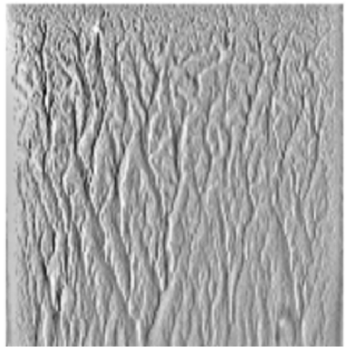
Figure 1: Pattern observed in erosion an experiment with commercial abrasive powder. Angles between $30^{\circ}$ and $90^{\circ}$ were found for different chevron alignments Daerr et al. (2003).

In this paper, we investigate through numerical simulation a physical model that is designed to represent the generic situation of flowing water on a plane composed of erodible sediment layer. This occurs naturally when the sea retreats from the shore or when a reservoir is drained. The flow of granular materials on planes is also of interest within the context of both industrial processing of powders and geophysical instabilities such as landslides and avalanches. These flows have been found to be complex, exhibiting several different flow regimes as well as particle segregation effects and instabilities Pouliquen et al. (1997). This paper is organized as follows. In Section II we describe the model used to simulate the erosion-deposition patterns. These patterns are presented and analysed in Section III, while the conclusions are left for Section IV.

Figure 2: A typical initial configuration of the regularized random network with $64$ grains and its corresponding triangulation.

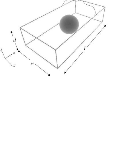
Figure 3: The velocity field is determined in the channel of length $l$ and width $w$ with one sphere of diameter $d$ inside. The mean velocity of the fluid $v_{f}$ is calculated in the rectangular cross-section.

II Model Formulation

We model a system that takes into account the interaction of a granular medium with an incompressible Newtonian fluid flowing through the corresponding pore space. The granular medium is initially considered as a $N\times N$ regularized random network (RRN) on a plane where the sites are the centers of mass of spherical grains with diameter $d$ that are totally submerged in a fluid (e.g., water). We initialize this network as a regular square where the distance between the closest neighbors is $l_{0}$. The points (centers of mass of the grains) are then moved randomly along vectors with arbitrary direction and random magnitude that are smaller than the distance between the points. In this way, the points are distributed randomly, but with a characteristic distance. More precisely, in order to avoid the occurrence of overlapping grains, the maximum value adopted for the modulus of these dislocation vectors is $(l_{0}-d)/2$. Although the lattice construction is made in $2D$, we are actually describing one layer of a three-dimensional system, since the centers of mass of the particles still lay on a $2D$ plane but the grains are considered to be spheres. This association will enable us to generate a network of capillaries representing a complex geometry of the pore space. At this point, the entire system is triangulated considering each grain as a vertex of a Voronoi tesselation. In Fig. 2 we show a typical initial RRN configuration and its corresponding triangulation

Next, we assume that the local pore geometry between each two nearest neighbors grains $i$ and $j$ in this lattice can be modeled as a capillary channel of length $l$ (the distance between barycenters of the corresponding adjacent triangles), height $d$ and width $w$ equal to the distance between their centers. As shown in Fig. 3, if we consider periodic boundary conditions (PBC) in the $x$-direction, such a channel should be equivalent to a parallelepiped of fluid containing in its center a solid sphere of diameter $d$ (grain).

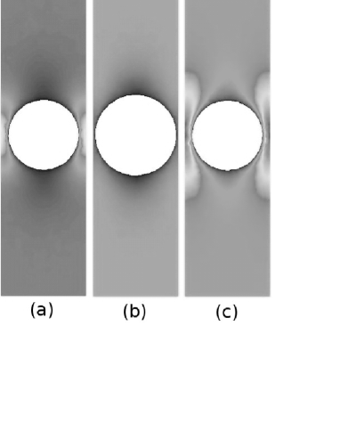
Figure 4: Contour plots of the velocity field obtained numerically for $w/d=1.05$ at three different transverse planes of the channel, namely, (a) $y/d=1/4$, (b) $y/d=1/2$ and (c) $y/d=3/4$. The gray shades ranging from dark to light correspond to low and high velocity magnitudes, respectively.

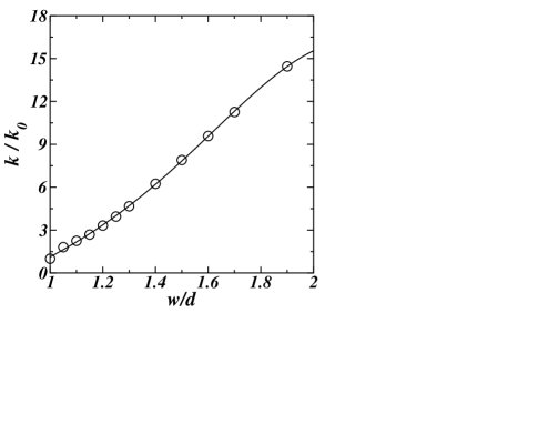
Figure 5: Permeability $\kappa$ versus the ratio $w/d$ for the local channel configuration shown in Fig. (3). Here $\kappa_{0}$ is the permeability for a channel with ratio $w/d=1$. The solid line is the best fit to the data of the fourth degree polynomial used to interpolate the local permeability of the channels in the pore network model.

Here the Navier-Stokes and continuity equations in the three-dimensional channel are solved using the commercial CFD software FLUENT flu . We consider no-slip boundary conditions at the bottom and assume that the top surface is shear-stress free. A pressure gradient $\Delta p$ is imposed between the two ends of the channel in the $z$-direction. Its magnitude is sufficiently small to ensure viscous flow conditions, i.e., a low Reynolds number regime of flow. We adopt a non-structured tetrahedral mesh to discretize the channel and an upwind finite-difference scheme is set to perform the numerical simulations. The steady-state velocity and pressure fields are calculated for different channel geometries by systematically varying the ratio $w/d$ in the range $1.05<w/d<1.9$.

In Figs. 4a-c we show three contour plots of the velocity field computed for a channel with porosity $w/d=1.05$ at heights $y/d=4$, $2$ and $3/4$, respectively. Considering the low Reynolds number conditions used in the simulations, the flow in the channel can be characterized in terms of a permeability index $\kappa$ through the relation,

$$v_{f}=-\frac{\kappa}{\mu}\frac{\Delta p}{\Delta z}~{},$$ (1)

where $\mu$ is the viscosity of the fluid and $v_{f}$ is the average flow velocity. In practical terms, once the velocity and pressure fields are obtained for a channel with a given value of $w/d$, we can compute the mean velocity value $v_{f}$ through a cross-section orthogonal to the flow in the system. By repeating this procedure for different values of the overall pressure drop $\Delta p$, we first confirm the validity of the linear relationship $v_{f}\propto\Delta p$ as expected from Eq. (1), so that the permeability $\kappa$ can be directly calculated from the slope of the corresponding straight line. As shown in Fig. 5, the dependence of $\kappa$ on the ratio $w/d$ can be fully described as $\kappa/\kappa_{0}=f(w/d)$ where $f(w/d)$ is a fourth degree polynomial of $w/d$ and $\kappa_{0}$ is the permeability for a channel with unitary aspect ratio, $w/d=1$.

Once the local geometry and permeability of all capillaries in the system is determined, we proceed by applying a constant pressure drop between the inlet and outlet, i.e., the top and bottom of the entire pore network. Periodic boundary conditions are assumed in the lateral direction of the network, and the following local mass conservation equations are imposed at each of their $N$ nodes to allow water flow throughout the entire pore space:

$$\sum_{j}g_{ij}(p_{i}-p_{j})=0~{}~{}\text{for}~{}~{}i=1,2,...,N~{},$$ (2)

where the index $j$ runs over all the neighbor nodes of node $i$, $g_{ij}\equiv wd\kappa/l$ is the hydraulic conductance of the pore and $p_{i}$ and $p_{j}$ are the pressures at nodes $i$ and $j$, respectively. Equation (2) corresponds to a set of $N^{2}$ coupled linear algebraic equations that are solved in terms of the nodal pressure field by means of a standard subroutine for sparse matrices. From the pressures in the nodes, the velocity magnitude of the fluid in each capillary can be computed.

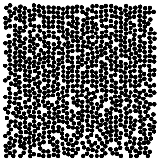
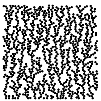
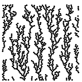
(a) (b) (c)

Figure 6: In (a), (b) and (c) we show the final configurations of the system for porosities $\phi$=$0.57$, $0.71$ and $0.80$, respectively after $11000$, $30000$ and $140000$ time steps. The grains arrange themselves in positions that give rise to characteristic patterns.

After the velocity field in the pore network is calculated, we allow each grain to move in the system. By assuming that there is no friction on the ground and drag is the only relevant force acting on the particles we obtain,

$${m\frac{d^{2}\bf{x}}{dt^{2}}}=3\pi\mu d\sum_{i}({\bf v}_{f}^{i}-{\bf v})~{}$$ (3)

where ${\bf v}_{f}^{i}$ is the fluid velocity at the channel i, $\bf{v}$ is the particle velocity, and the vectorial sum on the right is taken over all $n$ channels surrounding the particle. By straightforward integration of the equation of motion (3), the velocity and displacement caused by the fluid drag to each grain in the system during a time interval $\Delta t$ can be written as,

$${\bf v}=\frac{\sum_{i}{\bf v}_{f}^{i}}{n}-\left(\frac{\sum_{i}{\bf v}_{f}^{i}}{n}-{\bf v}_{0}\right)e^{-nC\Delta t}$$ (4)

$$\Delta{\bf x}=\frac{\sum_{i}{\bf v}_{f}^{i}}{n}\Delta t+\left(\frac{\sum_{i}{\bf v}_{f}^{i}}{n}-{\bf v}_{0}\right)\frac{e^{-nC\Delta t}}{nC}$$ (5)

where $C=18\mu/\rho d^{2}$, $\rho$ is the density of the grain, and ${\bf v}_{0}$ is its velocity in the previous time step.

In our simulations, the center of each grain is displaced by $\Delta{\bf{x}}$ using a time step $\Delta{t}$ that is sufficiently small to numerically ensure that the pattern evolution remains invariant when compared with results performed using even smaller time steps. The distance between the top and bottom lines of the system is kept constant with its center of mass moving according to the mean displacement of all grains. What is crucial for the steadiness of the pattern formation is that one grain cannot overlap with another grain. After computing the movement of all grains at each time step, the pore space is then modified, and we repeat the calculation of the velocity field to move the grains again, and so on. The simulation stops when the system reaches the steady-state, i.e., when the geometry of the aggregate remains unchanged with time.

III Results

We performed simulations on a lattice with $40\times 40$ grains with diameter $d=30\mu m$ and density $\rho=2.75g/cm^{3}$. These particles are surrounded by water, i.e., a fluid of viscosity $\mu=10^{-3}Pa.s$ which flows at small Reynolds conditions ($Re\ll 1$) through a pore space of porosity that can be varied in the range $0.6<\phi<0.8$. For each value of porosity we obtain results for five different realizations of the initial random pore space.

In Figs. 6a-c we show three final stable configurations of the model for different porosities values, $\phi$=$0.57$, $0.71$ and $0.80$, respectively. As can be observed, the steady-state patterns depend strongly on the porosity of the system. For sufficiently large values of $\phi$, the occurrence of particle clusters in the form of dendrites reflects the the strong coupling between fluid dynamics and grain movement, where the aligned preferential channels for flow leads to a high overall permeability of the porous system. For small porosities, however, no characteristic pattern is observed. This is to be expected since in compacted systems the grains do not have much mobility while in loose systems the particles have the freedom to move in almost all directions.

The tendency to form a dendritic pattern in which the particles align in preferential directions can be statistically quantified if we determine for each pair of grains the angle $\alpha$ between the line connecting their centers of mass and the direction orthogonal to the flow (i.e., the $x$-direction shown in Fig. 6a). In Figs. 7a-c we show the histograms of these angles $N(\alpha)$ for $\phi$=$0.57$, $0.71$ and $0.80$. For a low porosity system, $\phi=0.57$, the results shown in Fig. 7a indicate that a significant number of grains are aligned around $\alpha=25^{\circ}$ (and the symmetric direction of $155^{\circ}$), although the most frequent angle lies in the vicinity of $90^{\circ}$. This means that the particles tend to be aligned in the vertical $y$-direction (i.e., the direction of the flux), what is expected as the system cannot change much from its initial configuration. In systems with intermediate porosity values, $0.65<\phi<0.75$, there is a substantial change in the preferred angle of alignment, which is around $\alpha=60^{\circ}$ (and the symmetric direction of $120^{\circ}$). This behaviour, as exemplified here in Fig. 7b, resembles the chevron alignment reported in Ref. Daerr et al. (2003), where the results of the angle histograms are presented for a porosity $\phi=0.71$. In Fig. 7c we show the histogram $N(\alpha)$ for a large porosity system, $\phi=0.80$, where no evident preferential direction can be observed, with the particles aligning themselves in angles between $50^{\circ}$ and $130^{\circ}$, with approximately the same probability.

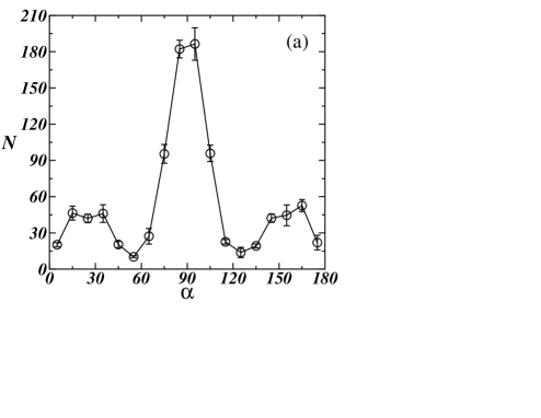
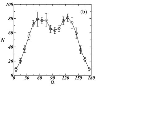
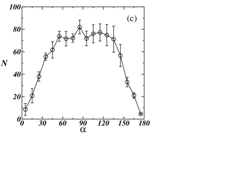
Figure 7: Histograms of pairs of grains that are touching and for which the line joining their centers of mass forms an angle $\alpha$ with the axis $x$. These results represent the average over five realizations of different porosities, namely, (a) $\phi=0.57$, (b) $0.71$ and (c) $0.80$.

Finally, it is important to investigate the flow properties of the porous system in terms of its macroscopic permeability $\kappa$ as a function of porosity. In Fig. 8 we show that, while the permeability increases very slowly with porosity for diluted systems (i.e., for low $\phi$ values), it augments in a rather sharp way at high values of $\phi$ to finally reach a divergent-like behavior in the vicinity of a porosity close to $\phi=0.8$. Interestingly, we find that this behavior can be well described by an inverse-logarithmic relation in the form $\kappa/\kappa_{0}=(a+b\ln{\phi})^{-1}$, as also depicted in Fig. 8.

IV Conclusions

We developed a numerical model to describe the process of erosion-deposition caused by laminar flow with the drag force given by the Stokes law. The results we obtained show the formation of a typical erosion pattern characterized by chevron alignments very similar to the experimental ones presented in Ref. Daerr et al. (2003) (a typical pattern is shown in Fig. 1). Through computational simulations performed with this model, we were able to find dendritic patterns as well as to reproduce the preferential alignment of the chevron structures observed in real experiments.

Our results indicate that these patterns depend substantially on the porosity of the system. Previous studies Geng et al. (2001); Reydellet and Clement (2001); Baxter et al. (1989) have shown that the size and shape of the particles influence dramatically the propagation of the fluid and the stress distribution in the system. Besides, it has been shown experimentally that the pattern geometry must also depend on the flow properties through the porous medium Andrade et al. (1995, 1999), namely, on whether or not the inertial mechanisms of momentum transport play an important role on the dynamics of pattern formation. In the present study we considered only laminar flow. By changing the exponent of the velocity in the drag law, for example, one can reproduce aspects of turbulent flow to increase the complexity in the movement of the particles. This could reveal a variety of new patterns. How the shape and the size distribution of the grains as well as the flow characteristics affect the patterns are natural questions that will be addressed in a future work.

In recent works Aranson et al. (2006); Borzsonyi et al. (2005); Malloggi et al. (2006), many patterns were observed in experiments involving avalanches, where one of the most important parameters is the depth of the substrate. Although the system studied here is related with erosion-sedimentation processes, this suggests that a variety of different patterns may be obtained just when one attempts to simulate them in three dimensions. A simple approximation to a three-dimensional system would be to consider that, depending on the flux, a particle would not stop as it reaches another particle, but could jump over it. With this possibility, the dynamics of the particles changes, as the velocity of them now depends also on the height of their centers of mass.

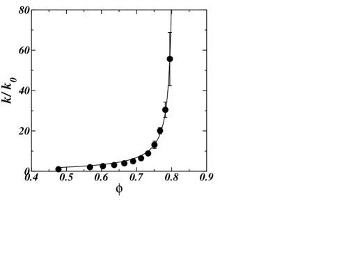
Figure 8: Dependence of the macroscopic permeability $\kappa$ at the steady-state on the porosity $\phi$ of the erosion-deposition system. The solid line is the best fit to the data of the function $\kappa/\kappa_{0}=(a+b\ln{\phi})^{-1}$, with parameters $a=-0.21$ and $b=-1.01$.

V Acknowledgements

We appreciate helpful interactions with A. M. C. Souza, A. A. P. Olarte, A. A. Moreira, and S. McNamara. This work was supported by the Brazilian agencies CNPq, CAPES and FUNCAP and Deutscher Akademischer Austauschdienst (DAAD). H. J. Herrmann thanks the Max-Planck prize.

References

- Behringer et al. (1999) R. Behringer, H. Jaeger, and S. Nagel, Chaos 9, 509 (1999).
- Jaeger et al. (1996) H. M. Jaeger, S. R. Nagel, and R. P. Behringer, Reviews of Modern Physics 68, 1259 (1996).
- Kroy et al. (2002) K. Kroy, G. Sauermann, and H. J. Herrmann, Phys. Rev. Lett. 88, 054301 (2002).
- Herrmann (1999) H. J. Herrmann, Physica A 263, 51 (1999).
- Ertas and Halsey (2002) D. Ertas and T. C. Halsey, Europh. Lett. 60, 931 (2002).
- Seybold et al. (2007) H. Seybold, J. S. Andrade, and H. J. Herrmann, PNAS 104, 16804 (2007).
- Daerr et al. (2003) A. Daerr, P. Lee, J. Lanuza, and E. Clement, Phys. Rev. E 67, 065201(R) (2003).
- Pouliquen (1999) O. Pouliquen, Physics of Fluids 11, 542 (1999).
- Aranson et al. (2006) I. S. Aranson, F. Malloggi, and E. Clement, Phys. Rev. E 73, 050302(R) (2006).
- Pouliquen and Vallance (1999) O. Pouliquen and J. W. Vallance, Chaos 9, 621 (1999).
- Borzsonyi et al. (2005) T. Borzsonyi, T. C. Halsey, and R. E. Ecke, Phys. Rev. Lett. 94, 208001 (2005).
- Forterre and Pouliquen (2003) Y. Forterre and O. Pouliquen, J. Fluid Mech. 486, 21 (2003).
- Pouliquen (2004) O. Pouliquen, Phys. Rev. Lett. 93, 248001 (2004).
- Midi (2004) G. D. R. Midi, Euro Phys. J. E 14, 341 (2004).
- Pouliquen et al. (1997) O. Pouliquen, J. Delour, and S. B. Savage, Letters to Nature 386, 816 (1997).
- (16) The FLUENT (trademark of FLUENT Inc.) fluid dynamics analysis package has been used in this study; http://www.fluent.com.
- Geng et al. (2001) J. Geng, D. Howell, E. Longhi, R. P. Behringer, G. Reydellet, L. Vanel, E. Clement, and S. Luding, Phys. Rev. Lett. 87, 035506 (2001).
- Reydellet and Clement (2001) G. Reydellet and E. Clement, Phys. Rev. Lett. 86, 3308 (2001).
- Baxter et al. (1989) G. W. Baxter, R. P. Behringer, T. Fagert, and G. A. Johnson, Phys. Rev. Lett. 62, 2825 (1989).
- Andrade et al. (1995) J. S. Andrade, D. A. Street, T. Shinohara, Y. Shibusa, and Y. Arai, Phys. Rev. E 51, 5725 (1995).
- Andrade et al. (1999) J. S. Andrade, U. M. S. Costa, M. P. Almeida, H. A. Makse, and H. E. Stanley, Phys. Rev. Lett. 82, 5249 (1999).
- Malloggi et al. (2006) F. Malloggi, J. Lanuza, B. Andreotti, and E. Clement, Europh. Lett. 75, 825 (2006).