Transport through a double-quantum-dot system with noncollinearly polarized leads

Abstract

We investigate linear and nonlinear transport in a double quantum dot system weakly coupled to spin-polarized leads. In the linear regime, the conductance as well as the nonequilibrium spin accumulation are evaluated in analytic form. The conductance as a function of the gate voltage exhibits four peaks of different height, with mirror symmetry with respect to the charge neutrality point. As the polarization angle is varied, due to exchange effects, the position and shape of the peaks change in a characteristic way which preserves the electron-hole symmetry of the problem. In the nonlinear regime various spin-blockade effects are observed. Moreover, negative differential conductance features occur for noncollinear magnetizations of the leads. In the considered sequential tunneling limit, the tunneling magnetoresistance (TMR) is always positive with a characteristic gate voltage dependence for noncollinear magnetization. If a magnetic field is added to the system, the TMR can become negative.

I Introduction

Spin-polarized transport through nanostructures is attracting increasing interest due to its potential application in spintronics Maekawa02 ; NJP07 as well as in quantum computing Awschalom02 . Downscaling magnetoelectronics devices to the nanoscale implies that Coulomb interaction effects become increasingly important Grabert92 ; Sohn97 . In particular, the interplay between spin-polarization and Coulomb blockade can give rise to a complex transport behavior in which both the spin and the charge of the ”information carrying” electron play a role. This has been widely demonstrated by many experimental studies on single-electron transistors (SETs) with ferromagnetic leads, with central element being either a ferromagnetic particle Ono97 ; Schelp97 ; Yakushiji05 , normal metal particles Zhang05 ; Bernand-Mantel06 , a two-level artificial molecule Pioro-Ladriere03 , a $C_{60}$ molecule Pasupathy04 , or a carbon nanotube Sahoo05 , showing the increasing complexity and variety of the investigated systems. Initially, the theoretical work was mainly focused on the difference in the transport properties for parallel or antiparallel magnetizations in generic spin-valve SETs Barnas98 ; Takahashi98 ; Majumdar98 ; Korotkov99 ; Brataas99 ; BrataasWang01 ; WeymannK nig05 ; Gorelik05 ; CottetChoi06 ; Fransson06b ; Weymann07 . More recently, the interplay between spin and interaction effects for noncollinear magnetization configurations has attracted quite some interest both in systems with a continuous energy spectrum Balents01 ; Bena02 ; Pedersen05 ; Wetzels05 , as well as in single-level quantum dots Sergueev02 ; K nig03 ; Braig05 ; Rudzinski05 ; Fransson05 ; Weymann05 ; Mu06 ; WeymannBarnas07 , many-level nanomagnets Parcollet06 and in carbon nanotubes quantum dots Koller07 . In the noncollinear case, a much richer physics is expected than in the collinear one. For example, two separate exchange effects have to be taken into account. On the one hand, there is the non-local interface exchange, in scattering theory for non-interacting systems described by the imaginary part of the spin-mixing conductance Brataas , and which in the context of current-induced magnetization dynamics acts as an effective field Stiles . Such an effective field has been found experimentally to strongly affect the transport dynamics in spin valves with MgO tunnel junctions Tulapurkar . This effect has recently also been involved to explain negative tunneling magnetoresistance effects in carbon nanotube spin valves Sahoo05 and called spin-dependent interface phase shifts Cottet06 ; CottetChoi06 . The second exchange term is an interaction-dependent exchange effect due to virtual tunneling processes that is absent in non-interacting systems Balents01 ; K nig03 ; Wetzels05 ; Koller07 . This latter exchange effect is potentially attractive for quantum information processing, since it allows to switch on and off magnetic fields in arbitrary directions just by a gate electric potential.

Figure 1: (Color online) Schematic picture of the model: A double quantum dot system attached to polarized leads. The significance of the on-site and inter-site interactions $U$ and $V$, respectively, is depicted. The source and drain contacts are polarized and the direction of the magnetizations $\vec{m}_{\alpha}$ is indicated by the arrows.

Recently, there has been increasing interest in double quantum dot systems realized e.g. in semiconducting structures Wiel03 or carbon nanotubes Gr ber06 , as tunable systems attractive for studying fundamental spin correlations. In fact the exchange Coulomb interaction induces a singlet-triplet splitting which can be used to perform logic gates Loss98 . Moreover, Coulomb interaction together with the Pauli principle can be used to induce spin-blockade when the two electrons have triplet correlations Ono02 ; Johnson05 ; Liu05 ; Fransson06 . The Pauli spin-blockade effect can be used to obtain a spin-polarized current even in the absence of spin-polarized leads; it requires a strong asymmetry between the two on-site energies of the left and right dot.

So far transport through a DD system with spin-polarized leads has been addressed in few theoretical Fransson06b ; Weymann07 ; tanaka and experimental Pioro-Ladriere03 works, for the case of collinearly polarized leads only. While Ref. Fransson06b addresses additional Pauli spin-blockade regimes when one lead is half-metallic and one is non-magnetic, Ref. Weymann07 focusses on the effects of higher order processes in symmetric DD systems, which can e.g. yield a zero bias anomaly or a negative tunneling magnetoresistance. In Pioro-Ladriere03 Coulomb blockade spectroscopy is used to measure the energy difference between symmetric and antisymmetric molecular states, and to determine the spin of the transferred electron.

In this work we investigate spin-dependent transport in the so-far unexplored case of a double-dot (DD) system connected to leads with arbitrary polarization direction. Specifically, we focus on the low transparency regime, where a weak coupling between the DD and the leads is assumed. Our model takes into account interface reflections as well as exchange effects due to the interactions and relevant for noncollinear polarization. We focus on the case of a symmetric DD, so that rectification effects induced by Pauli spin-blockade are excluded. In the linear transport regime the conductance is calculated in closed analytic form. This yields four distinct resonant tunneling regimes, but due to the electron-hole symmetry of the DD Hamiltonian, each posses a symmetric mirror with respect to the charge neutrality point. However, by applying an external magnetic field, this symmetry is broken, which can lead to negative tunneling magnetoresistance features. Finally, in the nonlinear regime some excitation lines can be suppressed for specific polarization angles, and negative differential features also occur.

The method developed in this work to investigate charge and spin transport is based on the Liouville equation for the reduced density matrix (RDM) in lowest order in the reflection and tunneling Hamiltonians. The obtained equations of motion are fully equivalent to those that could be obtained by using the Green’s function method K nig03 ; K nig96 in the same weak-tunneling limit. The advantage of our approach is that it is, in our opinion, easier to understand and to apply for newcomers, as it is based on standard perturbation theory and does not require knowledge of the nonequilibrium Green’s function formalism.

The paper is organized as follows. In Sec. II we introduce the model system for the ferromagnetic DD single-electron transistor. In Sec. III the coupled equations of motion for the elements of the DD reduced density matrix are derived. Readers not interested in the derivation of the dynamical equations can directly go to Secs. IV and V, where results for charge and spin transfer in the linear and nonlinear regime, respectively, are discussed. Finally, we present results for the transport characteristics in the presence of an external magnetic field in Sec. VI. Conclusions are drawn in Sec. VII.

II The model

We consider a two-level double-dot (DD), or a single molecule with two localized atomic orbitals, attached to ferromagnetic source and drain contacts and with a capacitive coupling to a lateral gate electrode. The system is described by the total Hamiltonian

$$\hat{H}=\hat{H}_{\odot}+\hat{H_{s}}+\hat{H_{d}}+\hat{H}_{T}+\hat{H}_{R},$$ (1)

accounting for the DD Hamiltonian, the source $(s)$ and drain $(d)$ leads, and the tunneling and reflection Hamiltonians, respectively. The two contacts are considered to be magnetized along an arbitrary, but fixed direction determined by the magnetization vectors $\vec{m}_{\alpha}$. The two magnetization axes enclose an angle $\Theta\in[0^{\circ},180^{\circ}]$ (see figure 1). The spin quantization axis $\vec{z}_{\alpha}$ in lead $\alpha$ is parallel to the magnetization $\vec{m}_{\alpha}$ of the lead. The majority of electrons in each contact will then be in the spin-up state. The Hamiltonians $\hat{H_{s}},\hat{H_{d}}$ that model the source ($s$) and drain ($d$) contacts read ($\alpha=s,d$)

$$\hat{H}_{\alpha}=\sum_{k\sigma_{\alpha}}(\varepsilon_{k\sigma_{\alpha}}-\mu_{\alpha})c^{\dagger}_{\alpha k\sigma_{\alpha}}c^{\phantom{\dagger}}_{\alpha k\sigma_{\alpha}},$$ (2)

where $c^{\dagger}_{\alpha k\sigma_{\alpha}}$ and $c^{\phantom{\dagger}}_{\alpha k\sigma_{\alpha}}$ are electronic lead operators. They create, respectively annihilate, electrons with momentum $k$ and spin $\sigma_{\alpha}$ in lead $\alpha$. The electrochemical potentials $\mu_{\alpha}=\mu_{0\alpha}+eV_{\alpha}$ contain the bias voltages $V_{s}$ and $V_{d}$ at the left and right lead with $V_{s}-V_{d}=V_{bias}$. There is no voltage drop within the DD. We denote in the following $\varepsilon_{k\sigma_{\alpha}}-\mu_{\alpha}:=\varepsilon_{\alpha k\sigma_{\alpha}}$.

Tunneling processes into and out of the DD are described by $\hat{H}_{T}$. We denote with $d^{\dagger}_{\alpha\sigma_{\alpha}}$, $d^{\phantom{\dagger}}_{\alpha\sigma_{\alpha}}$ the creation and destruction operators in the DD. We assume that tunneling only can happen between a contact and the closest dot, so that we can use the convention that to the leads indices $\alpha=s,d$ correspond $\alpha$ = 1,2 for the DD. With $t_{\alpha}$ the tunneling amplitude we find

$$\hat{H}_{T}=\sum_{\alpha k\sigma_{\alpha}}(t_{\alpha}d^{\dagger}_{\alpha\sigma_{\alpha}}c^{\phantom{\dagger}}_{\alpha k\sigma_{\alpha}}+{t_{\alpha}^{\ast}}c^{\dagger}_{\alpha k\sigma_{\alpha}}d^{\phantom{\dagger}}_{\alpha\sigma_{\alpha}}).$$ (3)

The so-called reflection-Hamiltonian $\hat{H}_{R}$ includes reflection events at the lead-molecule-interface Wetzels05 ; Koller07 . For strongly shielded leads the overall effect is the occurrence of a small energy shift $\Delta_{R}$, induced by the magnetic field in the contacts and built up during several cycles of reflections at the boundaries. It reads

$$\hat{H}_{R}=-\Delta_{R}\sum_{\alpha=s,d}(d^{\dagger}_{{\alpha}\uparrow_{\alpha}}d^{\phantom{\dagger}}_{{\alpha}\uparrow_{\alpha}}-d^{\dagger}_{{\alpha}\downarrow_{\alpha}}d^{\phantom{\dagger}}_{{\alpha}\downarrow_{\alpha}}).$$ (4)

Finally, the DD Hamiltonian needs to be specified. As spin quantization axis of the DD, $\vec{z}_{\odot}$, we choose the direction perpendicular to the plane spanned by $\vec{z}_{s}$ and $\vec{z}_{d}$ K nig03 (see Fig. 2). The two remaining basis vectors $\vec{x}_{\odot}$ and $\vec{y}_{\odot}$ are along $\vec{z}_{s}+\vec{z}_{d}$, respectively $\vec{z}_{s}-\vec{z}_{d}$.

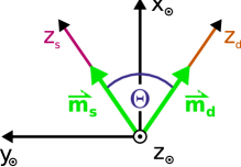
Figure 2: (Color online) The spin quantization axis of the double-dot, $z_{\odot}$, is chosen to be perpendicular to the plane spanned by the magnetization directions $\vec{m}_{s}$, $\vec{m}_{d}$ in the leads. The latter enclose an angle $\Theta$.

The matrices which mathematically describe the above transformations read

$$M_{s\leftrightarrow\odot}=\frac{1}{\sqrt{2}}\left(\begin{array}[]{cc}+e^{+i\Theta/4}&+e^{-i\Theta/4}\\ -e^{+i\Theta/4}&+e^{-i\Theta/4}\end{array}\right)=M_{d\leftrightarrow\odot}^{*}.$$ (5)

We express the DD Hamiltonian in the localized basis, such that e.g. $|+,-\rangle$ describes a state with a spin-up electron on site 1 and a spin down electron on site 2 (with spin directions expressed in the spin-coordinate system of the DD). Such state can be obtained by applying creation operators on the vacuum state, i.e., $|+,-\rangle=d^{\dagger}_{1\uparrow}d^{\dagger}_{2\downarrow}|0\rangle$. In general, the ordering of the creation operators is defined as $d^{\dagger}_{1\uparrow}d^{\dagger}_{2\uparrow}d^{\dagger}_{1\downarrow}d^{\dagger}_{2\downarrow}|0\rangle$. The DD Hamiltonian then reads

$$\hat{H}_{\odot} = \sum_{\alpha\sigma_{\odot}}\varepsilon_{\alpha}d^{\dagger}_{\alpha\sigma_{\odot}}d^{\phantom{\dagger}}_{\alpha\sigma_{\odot}}+b\sum_{\sigma_{\odot}}(d^{\dagger}_{1\sigma_{\odot}}d^{\phantom{\dagger}}_{2\sigma_{\odot}}+d^{\dagger}_{2\sigma_{\odot}}d^{\phantom{\dagger}}_{1\sigma_{\odot}})$$

$$+ (\xi-\frac{U}{2}-V)\sum_{\alpha=1}^{2}\sum_{\sigma_{\odot}}d^{\dagger}_{\alpha\sigma_{\odot}}d^{\phantom{\dagger}}_{\alpha\sigma_{\odot}}$$

$$+ U\sum_{\alpha=1}^{2}n_{\alpha\uparrow_{\odot}}n_{\alpha\downarrow_{\odot}}+V(n_{1\uparrow_{\odot}}+n_{1\downarrow_{\odot}})(n_{2\uparrow_{\odot}}+n_{2\downarrow_{\odot}}),$$

where the spin-index $\odot$ indicates that the operators are expressed in the spin-coordinate system of the DD. The tunneling coupling between the two sites is $b$, while $U$ and $V$ are on-site and inter-site Coulomb interactions. In the remaining we consider a symmetric DD with equal on site energies $\varepsilon_{1}=\varepsilon_{2}$. Thus we can incorporate the on-site energies in the parameter $\xi$ proportional to the applied gate voltage $V_{gate}$.

To understand transport properties of the two-site system in the weak tunneling regime, we have to analyze the eigenstates of the isolated interacting system. These states, expressed in terms of the localized states, and the corresponding eigenvalues are listed in table 1 Bulka04 . The table also indicates the eigenvalues of the total spin operator. The groundstates of the DD with odd particle number are spin degenerate. In contrast, the groundstates with even particle number have total spin $S=0$ and are not degenerate. In the case of the two particles groundstate the parameters $\alpha_{0}$ and $\beta_{0}$ determine whether the electrons prefer two pair in the same dot or are delocalized over the DD structure. Since the eigenstates are normalized to one, the condition $\alpha_{0}^{2}+\beta_{0}^{2}=1$ holds. The energy difference between the $S=0$ groundstate and the triplet is given by the exchange energy

$$J=\frac{1}{2}(\Delta-U+V)=2|b|(R+\sqrt{1+R^{2}})\,,$$

where $\Delta=4|b|\sqrt{1+R^{2}}$ and $R=(U-V)/(4|b|)$.
Besides the triplet, one observes the presence of higher two-particles excited states with total spin $S=0$.

Abbr.	State	Eigenvalue	Spin
$|0\rangle$	$|0,0\rangle$	0	$0$
$|1e\sigma\rangle$	$\frac{1}{\sqrt{2}}\left(|\sigma,0\rangle+|0,\sigma\rangle\right)$	$\xi^{\prime}+b$	$1/2$
$|1o\sigma\rangle$	$\frac{1}{\sqrt{2}}\left(|\sigma,0\rangle-|0,\sigma\rangle\right)$	$\xi^{\prime}-b$	$1/2$
$|2\rangle$	$\begin{array}[]{c}\frac{\alpha_{0}}{\sqrt{2}}\left(|+,-\rangle+|-,+\rangle\right)\\ +\frac{\beta_{0}}{\sqrt{2}}\left(|2,0\rangle+|0,2\rangle\right)\end{array}$	$2\xi^{\prime}+\frac{1}{2}(U+V-\Delta)$	$0$
$|2^{\prime}(1)\rangle$	$|+,+\rangle$
$|2^{\prime}(0)\rangle$	$\frac{1}{\sqrt{2}}\left(|+,-\rangle-|-,+\rangle\right)$	$2\xi^{\prime}+V$	$1$
$|2^{\prime}(-1)\rangle$	$|-,-\rangle$
$|2^{\prime\prime}\rangle$	$\frac{1}{\sqrt{2}}\left(|2,0\rangle-|0,2\rangle\right)$	$2\xi^{\prime}+U$	$0$
$|2^{\prime\prime\prime}\rangle$	$\begin{array}[]{c}\frac{\beta_{0}}{\sqrt{2}}\left(|+,-\rangle+|-,+\rangle\right)\\ -\frac{\alpha_{0}}{\sqrt{2}}\left(|2,0\rangle+|0,2\rangle\right)\end{array}$	$2\xi^{\prime}+\frac{1}{2}(U+V+\Delta)$	$0$
$|3o\sigma\rangle$	$\frac{1}{\sqrt{2}}\left(|2,\sigma\rangle+|\sigma,2\rangle\right)$	$3\xi^{\prime}+U+2V+b$	$1/2$
$|3e\sigma\rangle$	$\frac{1}{\sqrt{2}}\left(|2,\sigma\rangle-|\sigma,2\rangle\right)$	$3\xi^{\prime}+U+2V-b$	$1/2$
$|4\rangle$	$|2,2\rangle$	$4\xi^{\prime}+2U+4V$	$0$

in terms of $R=(U-V)/(4|b|)$:
$\Delta=4|b|\sqrt{1+R^{2}},\quad\alpha_{0}=\frac{1}{\sqrt{2}}\frac{1}{\sqrt{1+R^{2}-R\sqrt{1+R^{2}}}}$

Table 1: Eigenstates of the double-dot system and corresponding eigenvalues and parity. In the limit $|b|\to\infty$, where the inter-dot hopping is unhindered, $R\to 0$ and $\alpha_{0}\to\beta_{0}$. For $|b|\to 0$, i.e. no inter-dot hopping takes place, we find, if $U>V$, that $R\to+\infty$ and $\alpha_{0}\to 1$, $\beta_{0}\to 0$; the state $|2\rangle$ then becomes degenerate to $|2^{\prime}(0)\rangle$, forming a Heitler-London state. In turn, if $U<V$ then $R\to-\infty$ and $\alpha_{0}\to 0$, $\beta_{0}\to 1$.

Finally, we remark that $\hat{H}_{T}$ and $\hat{H}_{R}$ contain operators of the DD, $d^{\dagger}_{\alpha\sigma_{\alpha}}$ and $d^{\phantom{\dagger}}_{\alpha\sigma_{\alpha}}$, with spin quantization axis of the leads, while $\hat{H}_{\odot}$ is already expressed in terms of DD operators $d^{\dagger}_{\alpha\sigma_{\odot}}$ and $d^{\phantom{\dagger}}_{\alpha\sigma_{\odot}}$ with spin expressed in the coordinate system of the DD.

III Dynamical equations for the reduced density matrix

In this section we shortly outline how to derive the equation of motion for the reduced density matrix (RDM) to lowest non vanishing order in the tunneling and reflection Hamiltonians. The method is based on the well known Liouville equation for the total density matrix in lowest order in the tunneling and reflection Hamiltonian. Equations of motion for the reduced density matrix are obtained upon performing the trace over the leads degrees of freedom Blum96 , yielding, after standard approximations, Eqs. (III.1) and (14) below. In the case of spin-polarized leads, however, it is convenient to express the equations of motion for the RDM in the basis which diagonalizes the isolated system’s Hamiltonian and in the system’s spin quantization axis. After rotation from the leads quantization axis to the DD one, Eq. (21), which forms the basis of all the subsequent analysis, is obtained.

Let us start from the Liouville-equation for the total density matrix $\hat{\rho}^{I}(t)$ in the interaction-picture

$$i\hbar\frac{d\hat{\rho}^{I}(t)}{dt}=[\hat{H}^{I}_{T}(t)+\hat{H}^{I}_{R}(t),\hat{\rho}^{I}(t)],$$ (7)

with $\hat{H}_{T}$ and $\hat{H}_{R}$ transformed into the interaction picture by $\hat{H}^{I}_{T/R}(t)=e^{\frac{i}{\hbar}(\hat{H}_{\odot}+\hat{H}_{s}+\hat{H}_{d})(t-t_{0})}\quad\hat{H}_{T/R}\quad e^{-\frac{i}{\hbar}(\hat{H}_{\odot}+\hat{H}_{s}+\hat{H}_{d})(t-t_{0})}$, where $t_{0}$ indicates the time at which the perturbation is switched on. Integrating (7) over time and inserting the obtained expression in the r.h.s. of (7) one finds equivalently

$$\hat{\dot{\rho}}^{I}(t)=-\frac{i}{\hbar}[\hat{H}^{I}_{R}(t),\hat{\rho}^{I}(t_{0})]-\frac{i}{\hbar}[\hat{H}^{I}_{T}(t),\hat{\rho}^{I}(t_{0})]$$

$$- \frac{1}{\hbar^{2}}\int^{t}_{t_{0}}dt^{\prime}[\hat{H}^{I}_{T}(t)+\hat{H}^{I}_{R}(t),[\hat{H}^{I}_{T}(t^{\prime})+\hat{H}^{I}_{R}(t^{\prime}),\hat{\rho}^{I}(t^{\prime})]].$$

The time evolution of the reduced density matrix (RDM)

$$\hat{\rho}^{I}_{\odot}(t):=Tr_{leads}(\hat{\rho}^{I}(t))$$ (9)

is now formally obtained from (III) by tracing out the lead degrees of freedom. To proceed, we make the following standard approximations:

i) The leads are considered as reservoirs of non-interacting electrons which stay in thermal equilibrium at all times. In fact, we only consider weak tunneling and therefore the influence of the DD on the leads is marginal. Hence we can factorize the density matrix of the total system approximatively as

$$\hat{\rho}^{I}(t)\approx\hat{\rho}^{I}_{\odot}(t)\hat{\rho}_{s}\hat{\rho}_{d},$$ (10)

where $\rho_{s}$ and $\rho_{d}$ are time independent and given by the usual thermal equilibrium expression for the contacts $\hat{\rho}_{s/d}=\frac{e^{-\beta\hat{H}_{s/d}}}{Z_{s,d}}$, with $\beta$ being the inverse temperature and $Z_{s/d}$ the partition sums over all states of lead $s/d$.

ii) We consider the lowest non vanishing order in $\hat{H}_{T/R}$.

iii) We apply the Markov approximation, i.e., in the integral in Eq. (III) we replace $\hat{\rho}^{I}_{\odot}(t^{\prime})$ with $\hat{{\rho}}^{I}_{\odot}(t)$. In other words, it is assumed that the system looses all memory of its past due to the interaction with the leads electrons.

Furthermore, being interested in the long term behavior of the system only, we send $t_{0}\rightarrow-\infty$. We finally obtain the generalized master equation (GME) for the reduced density matrix

$$\hat{\dot{\rho}}^{I}_{\odot}(t)=-\frac{i}{\hbar}Tr_{leads}[\hat{H}^{I}_{R}(t),\hat{\rho}^{I}_{\odot}(t)\hat{\rho}_{s}\hat{\rho}_{d}]$$

$$- \frac{1}{\hbar^{2}}\int^{\infty}_{0}dt^{\prime\prime}Tr_{leads}\left([\hat{H}^{I}_{T}(t),[\hat{H}^{I}_{T}(t-t^{\prime\prime}),\hat{\rho}^{I}_{\odot}(t)\hat{\rho}_{s}\hat{\rho}_{d}]]\right).$$

III.1 Contribution from the tunneling Hamiltonian

In the following, we derive the explicit expression for the GME in the basis of the isolated DD. For simplicity we omit the contribution of the reflection Hamiltonian in a first instance. When we shall have obtained the final form of the GME due to the tunneling term, we will see that it is easy to insert the contribution from the reflection Hamiltonian. Let us then start from the tunneling Hamiltonian in the interaction picture

$$\hat{H}_{T}^{I}(t)=\sum_{\alpha k\sigma_{\alpha}}\sum_{i,j}$$

$$t_{\alpha}c^{\dagger}_{\alpha k\sigma_{\alpha}}(d^{\phantom{\dagger}}_{\alpha\sigma_{\alpha}})_{ij}\lvert i\rangle\langle j\lvert\exp\left[i(\varepsilon_{i}-\varepsilon_{j}+\varepsilon_{\alpha k\sigma_{\alpha}})t/\hbar\right]+h.c.$$

where $\big{(}d^{\phantom{\dagger}}_{\alpha\sigma_{\alpha}}\big{)}_{ij}=\langle i|d^{\phantom{\dagger}}_{\alpha\sigma_{\alpha}}|j\rangle$ and $\big{(}d^{\dagger}_{\alpha\sigma_{\alpha}}\big{)}_{ij}=\langle i|d^{\dagger}_{\alpha\sigma_{\alpha}}|j\rangle$ are the electron annihilation- and creation-operators in the spin-quantization axis of lead $\alpha$ expressed in the basis of the energy eigenstates of the quantum dot system. To simplify (III) standards approximations are invoked. i) The first one is the secular approximation: Fast oscillations in time average out in the stationary limit we are interested in, and thus can be neglected. Together with the relation $Tr_{leads}(\hat{\rho}_{s}\hat{\rho}_{d}c^{\dagger}_{\alpha k\sigma_{\alpha}}c_{\alpha^{\prime}k^{\prime}\sigma_{\alpha}^{\prime}})=\delta_{kk^{\prime}}\delta_{\alpha\alpha^{\prime}}\delta_{\sigma\sigma^{\prime}}f_{\alpha}(\varepsilon_{\alpha k\sigma}),$ where $f_{\alpha}(\varepsilon_{\alpha k\sigma})$ is the Fermi function, and the cyclic properties of the trace we get

$$\dot{\hat{\rho}}^{I}_{\odot}(t) = -\frac{1}{\hbar^{2}}\int^{\infty}_{0}dt^{\prime\prime}\sum_{\alpha k\sigma_{\alpha}}|{t_{\alpha}}|^{2}\left\{\right.$$

$$+\sum_{ilm}f_{\alpha}(\varepsilon_{\alpha k\sigma_{\alpha}})(d^{\phantom{\dagger}}_{\alpha\sigma_{\alpha}})_{il}(d^{\dagger}_{\alpha\sigma_{\alpha}})_{lm}\lvert i\rangle\langle m\lvert\hat{\rho}^{I}_{\odot}(t)\exp\left[i(\varepsilon_{m}-\varepsilon_{l}+\varepsilon_{\alpha k\sigma_{\alpha}})t^{\prime\prime}/\hbar\right]$$

$$+\sum_{ilm}(1-f_{\alpha}(\varepsilon_{\alpha k\sigma_{\alpha}}))(d^{\dagger}_{\alpha\sigma_{\alpha}})_{il}(d^{\phantom{\dagger}}_{\alpha\sigma_{\alpha}})_{lm}\lvert i\rangle\langle m\lvert\hat{\rho}^{I}_{\odot}(t)\exp\left[-i(\varepsilon_{l}-\varepsilon_{m}+\varepsilon_{\alpha k\sigma_{\alpha}})t^{\prime\prime}/\hbar\right]$$

$$+\sum_{ilm}f_{\alpha}(\varepsilon_{\alpha k\sigma_{\alpha}})\hat{\rho}^{I}_{\odot}(t)(d^{\phantom{\dagger}}_{\alpha\sigma_{\alpha}})_{il}(d^{\dagger}_{\alpha\sigma_{\alpha}})_{lm}\lvert i\rangle\langle m\lvert\exp\left[-i(\varepsilon_{i}-\varepsilon_{l}+\varepsilon_{\alpha k\sigma_{\alpha}})t^{\prime\prime}/\hbar\right]$$

$$+\sum_{ilm}(1-f_{\alpha}(\varepsilon_{\alpha k\sigma_{\alpha}}))\hat{\rho}^{I}_{\odot}(t)(d^{\dagger}_{\alpha\sigma_{\alpha}})_{il}(d^{\phantom{\dagger}}_{\alpha\sigma_{\alpha}})_{lm}\lvert i\rangle\langle m\lvert\exp\left[+i(\varepsilon_{l}-\varepsilon_{i}+\varepsilon_{\alpha k\sigma_{\alpha}})t^{\prime\prime}/\hbar\right]$$

$$-\sum_{iljm}(1-f_{\alpha}(\varepsilon_{\alpha k\sigma_{\alpha}}))(d^{\phantom{\dagger}}_{\alpha\sigma_{\alpha}})_{ij}\hat{\rho}^{I}_{\odot}(t)_{jl}(d^{\dagger}_{\alpha\sigma_{\alpha}})_{lm}\lvert i\rangle\langle m\lvert\exp\left[+i(\varepsilon_{m}-\varepsilon_{l}+\varepsilon_{\alpha k\sigma_{\alpha}})t^{\prime\prime}/\hbar\right]$$

$$-\sum_{iljm}f_{\alpha}(\varepsilon_{\alpha k\sigma_{\alpha}})(d^{\dagger}_{\alpha\sigma_{\alpha}})_{ij}\hat{\rho}^{I}_{\odot}(t)_{jl}(d^{\phantom{\dagger}}_{\alpha\sigma_{\alpha}})_{lm}\lvert i\rangle\langle m\lvert\exp\left[-i(\varepsilon_{l}-\varepsilon_{m}+\varepsilon_{\alpha k\sigma_{\alpha}})t^{\prime\prime}/\hbar\right]$$

$$-\sum_{iljm}(1-f_{\alpha}(\varepsilon_{\alpha k\sigma_{\alpha}}))(d^{\phantom{\dagger}}_{\alpha\sigma_{\alpha}})_{ij}\hat{\rho}^{I}_{\odot}(t)_{jl}(d^{\dagger}_{\alpha\sigma_{\alpha}})_{lm}\lvert i\rangle\langle m\lvert\exp\left[-i(\varepsilon_{i}-\varepsilon_{j}+\varepsilon_{\alpha k\sigma_{\alpha}})t^{\prime\prime}/\hbar\right]$$

$$-\sum_{iljm}f_{\alpha}(\varepsilon_{\alpha k\sigma_{\alpha}})(d^{\dagger}_{\alpha\sigma_{\alpha}})_{ij}\hat{\rho}^{I}_{\odot}(t)_{jl}(d^{\phantom{\dagger}}_{\alpha\sigma_{\alpha}})_{lm}\lvert i\rangle\langle m\lvert\exp\left[+i(\varepsilon_{j}-\varepsilon_{i}+\varepsilon_{\alpha k\sigma_{\alpha}})t^{\prime\prime}/\hbar\right]\left.\right\}.$$

ii) For the second approximation we notice that we wish to evaluate single components $\langle n\lvert\hat{\rho}_{\odot}^{I}\lvert m\rangle$ of the RDM in the system’s energy eigenbasis. Therefore, we assume that the DD is in a pure charge state with a certain number of electrons $N$ and energy $E_{N}$ . In fact, in the weak tunneling limit the time between two tunneling events is longer than the time where relaxation processes happen. That is, we can neglect matrix elements between states with different number of electrons, and only regard elements of $\hat{\rho}_{\odot}^{I}$ which connect states with same electron number $N$ and same energy $E_{N}$. So we can divide $\hat{\rho}_{\odot}^{I}$ into sub-matrices labelled with $N$ and $E_{N}$ and find

$$\dot{{\rho}}^{E_{N}N}_{{nm}}(t)=-\frac{\pi}{\hbar}\sum_{\alpha\sigma_{\alpha}}\quad\left\{\sum_{l,l^{\prime}\in{\lvert N-1\rangle}},\quad\sum_{j\in\lvert E_{N}N\rangle},\quad\sum_{h,h^{\prime}\in{\lvert N+1\rangle}}\right\}|{t_{\alpha}}|^{2}\left\{\right.$$ (14)

$$\mathrm{(a)} +\left[f_{\alpha}(\varepsilon_{h}-\varepsilon_{j})D_{\alpha\sigma_{\alpha}}(\varepsilon_{h}-\varepsilon_{j})+\frac{i}{\pi}\int^{\prime}d\varepsilon_{k}\frac{f_{\alpha}(\varepsilon_{k})D_{\alpha\sigma_{\alpha}}(\varepsilon_{k})}{\varepsilon_{k}-\varepsilon_{h}+\varepsilon_{j}}\right](d^{\phantom{\dagger}}_{\alpha\sigma_{\alpha}})_{nh}(d^{\dagger}_{\alpha\sigma_{\alpha}})_{hj}{\rho}^{E_{N}N}_{{jm}}(t)$$

$$\mathrm{(b)} +\left[\left(1-f_{\alpha}(\varepsilon_{j}-\varepsilon_{l})\right)D_{\alpha\sigma_{\alpha}}(\varepsilon_{j}-\varepsilon_{l})-\frac{i}{\pi}\int^{\prime}d\varepsilon_{k}\frac{\left(1-f_{\alpha}(\varepsilon_{k})\right)D_{\alpha\sigma_{\alpha}}(\varepsilon_{k})}{\varepsilon_{k}-\varepsilon_{j}+\varepsilon_{l}}\right](d^{\dagger}_{\alpha\sigma_{\alpha}})_{nl}(d^{\phantom{\dagger}}_{\alpha\sigma_{\alpha}})_{lj}{\rho}^{E_{N}N}_{{jm}}(t)$$

$$\mathrm{(c)} +\left[f_{\alpha}(\varepsilon_{h}-\varepsilon_{j})D_{\alpha\sigma_{\alpha}}(\varepsilon_{h}-\varepsilon_{j})-\frac{i}{\pi}\int^{\prime}d\varepsilon_{k}\frac{f_{\alpha}(\varepsilon_{k})D_{\alpha\sigma_{\alpha}}(\varepsilon_{k})}{\varepsilon_{k}-\varepsilon_{h}+\varepsilon_{j}}\right]{\rho}^{E_{N}N}_{{nj}}(t)(d_{\alpha\sigma_{\alpha}})_{jh}(d^{\dagger}_{\alpha\sigma_{\alpha}})_{hm}$$

$$\mathrm{(d)} +\left[\left(1-f_{\alpha}(\varepsilon_{j}-\varepsilon_{l})\right)D_{\alpha\sigma_{\alpha}}(\varepsilon_{j}-\varepsilon_{l})+\frac{i}{\pi}\int^{\prime}d\varepsilon_{k}\frac{\left(1-f_{\alpha}(\varepsilon_{k})\right)D_{\alpha\sigma_{\alpha}}(\varepsilon_{k})}{\varepsilon_{k}-\varepsilon_{j}+\varepsilon_{l}}\right]{\rho}^{E_{N}N}_{{nj}}(t)(d^{\dagger}_{\alpha\sigma_{\alpha}})_{jl}(d^{\phantom{\dagger}}_{\alpha\sigma_{\alpha}})_{lm}$$

$$\mathrm{(e)} -2\left(1-f_{\alpha}(\varepsilon_{h}-\varepsilon_{j})\right)D_{\alpha\sigma_{\alpha}}(\varepsilon_{h}-\varepsilon_{j})(d^{\phantom{\dagger}}_{\alpha\sigma_{\alpha}})_{nh^{\prime}}(d^{\dagger}_{\alpha\sigma_{\alpha}})_{hm}{\rho}^{E_{h}N+1}_{{h^{\prime}h}}(t)$$

$$\mathrm{(f)} -2f_{\alpha}(\varepsilon_{j}-\varepsilon_{l})D_{\alpha\sigma_{\alpha}}(\varepsilon_{j}-\varepsilon_{l})(d^{\dagger}_{\alpha\sigma_{\alpha}})_{nl^{\prime}}(d^{\phantom{\dagger}}_{\alpha\sigma_{\alpha}})_{lm}{\rho}^{E_{l}N-1}_{{l^{\prime}l}}(t)\left.\right\}.$$

In (14) we used the notation ${\rho}^{E_{N}N}_{nm}:=\langle n|{\hat{\rho}}^{I,E_{N}N}_{\odot}|m\rangle$.
By convention, $\{\sum_{l,l^{\prime}},\sum_{j},\sum_{h,h^{\prime}}\}$ means that in each line (a)-(f) we sum over the indices occurring in this line only. Notice that the sum over $j$ is restricted to states of energy $E_{j}=E_{N}=E_{n}=E_{m}$. For the states with $N\pm 1$ electrons, we have to sum over all energies, therefore we indexed the density matrix with $E_{h}=E_{h^{\prime}}$ respectively $E_{l}=E_{l^{\prime}}$ in lines (e) and (f). Further, we replaced the sum over $k$ by an integral: $\sum_{k}\longrightarrow\int d\varepsilon_{\alpha k\sigma_{\alpha}}D_{\alpha\sigma_{\alpha}}(\varepsilon_{\alpha k\sigma_{\alpha}})$, where $D_{\alpha\sigma_{\alpha}}(\varepsilon_{\alpha k\sigma_{\alpha}})$ denotes the density of states in lead $\alpha$ for the spin direction $\sigma_{\alpha}$, and applied the useful formula

$$\int d\varepsilon_{\alpha k\sigma_{\alpha}}G(\varepsilon_{\alpha k\sigma_{\alpha}})\int_{0}^{t}dt^{\prime\prime}e^{\pm\frac{i}{\hbar}(\varepsilon_{\alpha k\sigma_{\alpha}}-E)t^{\prime\prime}}$$

$$=\pi\hbar G(E)\pm i\hbar\int^{\prime}d\varepsilon_{\alpha k\sigma_{\alpha}}\frac{G(\varepsilon_{\alpha k\sigma_{\alpha}})}{(\varepsilon_{\alpha k\sigma_{\alpha}}-E)}\;,$$ (15)

where the prime at the integral denotes Cauchy’s principal part integration. In our case $G(\varepsilon_{\alpha k\sigma_{\alpha}})=D_{\alpha\sigma_{\alpha}}(\varepsilon_{\alpha k\sigma_{\alpha}})f^{\pm}_{\alpha}(\varepsilon_{\alpha k\sigma_{\alpha}})$ with $f^{+}_{\alpha}=f_{\alpha}$ and $f^{-}_{\alpha}=1-f_{\alpha}$. In order to simplify the notations we replaced $\varepsilon_{\alpha k\sigma_{\alpha}}$ by $\varepsilon_{k}$ in (14).

III.2 Transformation into the spin coordinate system of the double-dot

In the previous section we introduced the transformation rules for changing from the lead spin coordinates $\sigma_{\alpha}$ into the DD spin coordinates $\sigma_{\odot}$. These rules give

$$\left(\begin{array}[]{c}d^{\dagger}_{\alpha\uparrow_{\alpha}}\\ d^{\dagger}_{\alpha\downarrow_{\alpha}}\end{array}\right)=\frac{1}{\sqrt{2}}\left(\begin{array}[]{cc}+e^{-i\Theta_{\alpha}/2}&+e^{+i\Theta_{\alpha}/2}\\ -e^{-i\Theta_{\alpha}/2}&+e^{+i\Theta_{\alpha}/2}\end{array}\right)\left(\begin{array}[]{c}d^{\dagger}_{\alpha\uparrow_{\odot}}\\ d^{\dagger}_{\alpha\downarrow_{\odot}}\end{array}\right)$$ (16)

with $\Theta_{s}:=-\frac{\Theta}{2}$, $\Theta_{d}:=+\frac{\Theta}{2}$.
Thus, Eq. (14) can be easily expressed in the DD spin quantization axis. For example it holds

$$\sum_{\sigma_{\alpha}}D_{\alpha\sigma_{\alpha}}d^{\dagger}_{\sigma_{\alpha}}d_{\sigma_{\alpha}}=$$

$$\frac{1}{2}\left(D_{\alpha\uparrow_{\alpha}}+D_{\alpha\downarrow_{\alpha}}\right)\sum_{\sigma_{\odot}}\Phi_{\alpha\sigma_{\odot}\sigma_{\odot}}d^{\dagger}_{\alpha\sigma_{\odot}}d^{\phantom{\dagger}}_{\alpha\sigma_{\odot}}$$

$$+ \frac{1}{2}\left(D_{\alpha\uparrow_{\alpha}}-D_{\alpha\downarrow_{\alpha}}\right)\sum_{\sigma_{\odot}}\Phi^{*}_{\alpha\sigma_{\odot}-\sigma_{\odot}}d^{\dagger}_{\alpha\sigma_{\odot}}d^{\phantom{\dagger}}_{\alpha-\sigma_{\odot}}$$

where we introduced

$$\Phi_{\alpha\sigma_{\odot}\sigma_{\odot}^{\prime}}:=\left\{\begin{array}[]{l@{\qquad}r}1&\sigma_{\odot}=\sigma_{\odot}^{\prime}\;,\\ e^{i\Theta_{\alpha}}&\sigma_{\odot}=\uparrow\quad\sigma_{\odot}^{\prime}=\downarrow\;,\\ e^{-i\Theta_{\alpha}}&\sigma_{\odot}=\downarrow\quad\sigma_{\odot}^{\prime}=\uparrow\;.\\ \end{array}\right.$$

For later convenience we also define

$$F^{\pm}_{\alpha\sigma_{\odot}\sigma_{\odot}^{\prime}}:=\frac{1}{2}\left\{\begin{array}[]{l@{\qquad}r}D_{\alpha+_{\alpha}}f^{\pm}_{\alpha}(E)+D_{\alpha-_{\alpha}}f^{\pm}_{\alpha}(E)&\sigma_{\odot}=\sigma_{\odot}^{\prime},\\ D_{\alpha+_{\alpha}}f^{\pm}_{\alpha}(E)-D_{\alpha-_{\alpha}}f^{\pm}_{\alpha}(E)&\sigma_{\odot}\neq\sigma_{\odot}^{\prime},\end{array}\right.$$

and its related principal part integral

$$P^{\pm}_{\alpha\sigma_{\odot}\sigma_{\odot}^{\prime}}(E):=\int^{\prime}d{\varepsilon}F^{\pm}_{\alpha\sigma_{\odot}\sigma_{\odot}^{\prime}}(\varepsilon)(\varepsilon-E)^{-1}.$$

III.3 Contribution from the reflection Hamiltonian

In order to give the full expression for the GME in the system’s eigenbasis, we need to compute the contribution from the reflection Hamiltonian in Eq. (III). In analogy to what we did to evaluate the contribution from the tunneling Hamiltonian, we must first transform $\hat{H}_{R}$ into the interaction picture and then perform the secular approximation to get rid of the time-dependence. To start, we express $\hat{H}_{R}$ in the DD spin quantization basis,

$$\hat{H}^{I}_{R} = -\Delta_{R}\sum_{\alpha}\sum_{\begin{subarray}{c}j\in\lvert N\rangle\\ l\in\lvert N-1\rangle\end{subarray}}\sum_{\sigma_{\odot}\neq\sigma_{\odot}^{\prime}}\Phi^{\ast}_{\alpha\sigma_{\odot}\sigma_{\odot}^{\prime}}{d^{\dagger}_{\sigma_{\odot}}}_{jl}{d_{\sigma_{\odot}^{\prime}}}_{lj}\lvert j\rangle\langle j\lvert.$$

The commutator is easily evaluated to be

$$-\frac{i}{\hbar}Tr_{leads}[\hat{H}^{I}_{R},\hat{\rho}^{I}_{\odot}(t)\rho_{s}\rho_{d}]=$$ (19)

$$-\frac{i}{\hbar}\sum_{\alpha}\Delta_{R}\sum_{j\in\lvert N\rangle}\sum_{l\in\lvert N-1\rangle}\sum_{\sigma_{\odot}\neq\sigma_{\odot}^{\prime}}\Phi^{\ast}_{\alpha\sigma_{\odot}\sigma_{\odot}^{\prime}}$$

$$\left[{d^{\dagger}_{\sigma_{\odot}}}_{jl}{d_{\sigma_{\odot}^{\prime}}}_{lj}\lvert j\rangle\langle j\lvert\hat{\rho}^{I}_{\odot}(t)-\hat{\rho}^{I}_{\odot}(t){d^{\dagger}_{\sigma_{\odot}}}_{jl}{d_{\sigma_{\odot}^{\prime}}}_{lj}\lvert j\rangle\langle j\lvert\right].$$

In order to include this commutator in the master equation (14) let us introduce the abbreviation

$$R_{\alpha\sigma_{\odot}\sigma_{\odot}^{\prime}}=\frac{1}{|{t^{\alpha}}|^{2}}\Delta_{R}\left(\delta_{\sigma_{\odot}\uparrow}\delta_{\sigma_{\odot}^{\prime}\downarrow}+\delta_{\sigma_{\odot}\downarrow}\delta_{\sigma_{\odot}^{\prime}\uparrow}\right).$$ (20)

Now we can add $R_{\alpha\sigma_{\odot}\sigma_{\odot}^{\prime}}$ in (14) in the lines ($b$) and ($d$) to find the final form of the complete master equation in the DD spin-coordinate system. It reads

$$\dot{{\rho}}_{nm}^{E_{N}N}(t)=-\frac{\pi}{\hbar}\sum_{\alpha=s,d}|{t^{\alpha}}|^{2}\sum_{\sigma_{\odot},\sigma\odot^{\prime}}\left\{\sum_{l,l^{\prime}\in{\lvert N-1\rangle}},\quad\sum_{j\in\lvert E_{N}N\rangle},\quad\sum_{h,h^{\prime}\in{\lvert N+1\rangle}}\right\}\left\{\right.$$ (21)

$$\mathrm{(a)} +\Phi_{\alpha\sigma_{\odot}\sigma_{\odot}^{\prime}}\big{[}F^{+}_{\alpha\sigma_{\odot}\sigma_{\odot}^{\prime}}(\varepsilon_{h}-\varepsilon_{j})+\frac{i}{\pi}P^{+}_{\alpha\sigma_{\odot}\sigma_{\odot}^{\prime}}(\varepsilon_{h}-\varepsilon_{j})\big{]}\big{(}d_{\alpha\sigma_{\odot}}\big{)}_{nh}\big{(}d^{\dagger}_{\alpha\sigma_{\odot}^{\prime}}\big{)}_{hj}\;{\rho}_{jm}^{E_{N}N}(t)$$

$$\mathrm{(b)} +\Phi^{\ast}_{\alpha\sigma_{\odot}\sigma_{\odot}^{\prime}}\Big{[}F^{-}_{\alpha\sigma_{\odot}\sigma_{\odot}^{\prime}}(\varepsilon_{j}-\varepsilon_{l})-\frac{i}{\pi}\left[P^{-}_{\alpha\sigma_{\odot}\sigma_{\odot}^{\prime}}(\varepsilon_{j}-\varepsilon_{l})+R_{\alpha\sigma_{\odot}\sigma^{\prime}_{\odot}}\right]\Big{]}\big{(}d^{\dagger}_{\alpha\sigma_{\odot}}\big{)}_{nl}\big{(}d_{\alpha\sigma_{\odot}^{\prime}}\big{)}_{lj}{\rho}_{jm}^{E_{N}N}(t)$$

$$\mathrm{(c)} +\Phi_{\alpha\sigma_{\odot}\sigma_{\odot}^{\prime}}\big{[}F^{+}_{\alpha\sigma_{\odot}\sigma_{\odot}^{\prime}}(\varepsilon_{h}-\varepsilon_{j})-\frac{i}{\pi}P^{+}_{\alpha\sigma_{\odot}\sigma_{\odot}^{\prime}}(\varepsilon_{h}-\varepsilon_{j})\big{]}{\rho}_{nj}^{E_{N}N}(t)\big{(}d_{\alpha\sigma_{\odot}}\big{)}_{jh}\big{(}d^{\dagger}_{\alpha\sigma_{\odot}^{\prime}}\big{)}_{hm}$$

$$\mathrm{(d)} +\Phi^{\ast}_{\alpha\sigma_{\odot}\sigma_{\odot}^{\prime}}\Big{[}F^{-}_{\alpha\sigma_{\odot}\sigma_{\odot}^{\prime}}(\varepsilon_{j}-\varepsilon_{l})+\frac{i}{\pi}\left[P^{-}_{\alpha\sigma_{\odot}\sigma_{\odot}^{\prime}}(\varepsilon_{j}-\varepsilon_{l})+R_{\alpha\sigma_{\odot}\sigma^{\prime}_{\odot}}\right]\Big{]}{\rho}_{nj}^{E_{N}N}(t)\big{(}d^{\dagger}_{\alpha\sigma_{\odot}}\big{)}_{jl}\big{(}d_{\alpha\sigma_{\odot}^{\prime}}\big{)}_{lm}$$

$$\mathrm{(e)} -2\Phi_{\alpha\sigma_{\odot}\sigma_{\odot}^{\prime}}F^{-}_{\alpha\sigma_{\odot}\sigma_{\odot}^{\prime}}(\varepsilon_{h}-\varepsilon_{j})\big{(}d_{\alpha\sigma_{\odot}}\big{)}_{nh^{\prime}}\rho_{h^{\prime}h}^{E_{h}N+1}(t)\big{(}d^{\dagger}_{\alpha\sigma_{\odot}^{\prime}}\big{)}_{hm}$$

$$\mathrm{(f)} -2\Phi^{\ast}_{\alpha\sigma_{\odot}\sigma_{\odot}^{\prime}}F^{+}_{\alpha\sigma_{\odot}\sigma_{\odot}^{\prime}}(\varepsilon_{j}-\varepsilon_{l})\big{(}d^{\dagger}_{\alpha\sigma_{\odot}}\big{)}_{nl^{\prime}}\rho_{l^{\prime}l}^{E_{l}N-1}(t)\big{(}d_{\alpha\sigma_{\odot}^{\prime}}\big{)}_{lm}\left.\right\}.$$

III.4 The current formula

We observe now that (21) can be recast in the Bloch-Redfield form

$$\dot{\rho}_{nm}^{E_{N}N}(t) = -\sum_{jj^{\prime}}R_{nm\,jj^{\prime}}^{NN}\ \rho_{jj^{\prime}}^{E_{N}N}(t)$$ (22)

$$+\sum_{hh^{\prime}}R_{nm\,hh^{\prime}}^{N\,N+1}\rho_{hh^{\prime}}^{E_{h}N+1}(t)$$

$$+\sum_{ll^{\prime}}R_{nm\,ll^{\prime}}^{N\,N-1}\rho_{ll^{\prime}}^{E_{l}N-1}(t),$$

where the sums in (22) run over states with fixed particle number: $j,j^{\prime}\in\{\left|E_{N}N\right.\rangle\}$, $h,h^{\prime}\in\{\left|N+1\right.\rangle\}$, $l,l^{\prime}\in\{\left|N-1\right.\rangle\}$. The Redfield tensors are given by $(\alpha=s,d)$ Koller07

$$R_{nm\,jj^{\prime}}^{NN} = \sum_{\alpha}\sum_{l(\texttt{or}\;h)}\left[\delta_{mj^{\prime}}\left(\Gamma_{\alpha,nhhj}^{(+)N\,N+1}+\Gamma_{\alpha,nllj}^{(+)N\,N-1}\right)\right.$$ (23)

$$+\left.\delta_{nj}\left(\Gamma_{\alpha,j^{\prime}hhm}^{(-)NN+1}+\Gamma_{\alpha,j^{\prime}llm}^{(-)NN-1}\right)\right],$$

$$R_{nm\,kk^{\prime}}^{N\,N\pm 1}=\sum_{\alpha}\left(\Gamma_{\alpha,k^{\prime}mnk}^{(+)NN\mp 1}+\Gamma_{\alpha,k^{\prime}mnk}^{(-)NN\mp 1}\right),$$ (24)

where the quantities $\Gamma_{\alpha,njjk}^{(\pm)N\,N\pm 1}$ can be easily read out from (21). They are

$$\Gamma_{\alpha,nhh^{\prime}k}^{(\pm)NN+1} = \sum_{\sigma_{\odot}\sigma^{\prime}_{\odot}}\{\frac{\pi}{\hbar}\Phi_{\alpha\sigma_{\odot}\sigma^{\prime}_{\odot}}|t_{\alpha}|^{2}[F^{+}_{\alpha\sigma_{\odot}\sigma^{\prime}_{\odot}}(\varepsilon_{h}-\varepsilon_{k})$$

$$\pm \frac{i}{\pi}P^{+}_{\alpha\sigma\sigma^{\prime}}(\varepsilon_{h}-\varepsilon_{k})](d_{\alpha\sigma_{\odot}})_{nh}(d^{\dagger}_{\alpha\sigma^{\prime}_{\odot}})_{h^{\prime}k}\},$$

$$\Gamma_{\alpha,nll^{\prime}k}^{(\pm)NN-1}=\sum_{\sigma_{\odot}\sigma^{\prime}_{\odot}}\{\frac{\pi}{\hbar}\Phi^{*}_{\alpha\sigma_{\odot}\sigma^{\prime}_{\odot}}|t_{\alpha}|^{2}[F^{-}_{\alpha\sigma_{\odot}\sigma^{\prime}_{\odot}}(\varepsilon_{k}-\varepsilon_{l})$$

$$\mp \frac{i}{\pi}(P^{-}_{\alpha\sigma_{\odot}\sigma^{\prime}_{\odot}}(\varepsilon_{k}-\varepsilon_{l})+R_{\alpha\sigma_{\odot}\sigma^{\prime}_{\odot}})](d^{\dagger}_{\alpha\sigma_{\odot}})_{nl}(d_{\alpha\sigma^{\prime}_{\odot}})_{l^{\prime}k}\}\;.$$

With the stationary density matrix $\hat{\rho}_{\odot st}^{I}$ being known, the current (through lead $\alpha=s/d=\pm$) follows from

$$I=2\alpha e{\rm Re}\sum_{N}\sum_{n,n^{\prime},j}\left(\Gamma_{\alpha,njjn^{\prime}}^{(+)N\,{N+1}}-\Gamma_{\alpha,njjn^{\prime}}^{(+)N\,{N-1}}\right)\rho_{n^{\prime}n,st}^{E_{n}N}.$$ (25)

We solve Eq. (22) numerically and use the result to evaluate the current flowing through the DD, as shown in the forthcoming sections. At low bias voltages, however, we can make some further approximations to arrive at an analytical formula for the static DC current.

IV The low-bias regime

IV.1 General considerations

A low bias voltage ensures that merely one channel is involved with respect to transport properties. Here we focus on gate voltages which align charge states $N$ and $N+1$. Moreover, we can focus on density matrix elements which involve the energy ground states $E_{N}^{(0)}$ and $E_{N+1}^{(0)}$ only. In the following we shall use the compact notations

$$\hat{\rho}_{\odot}^{I,E_{N}^{(0)}N}:=\hat{\rho}_{\odot}^{(N)};\quad\langle n|\hat{\rho}_{\odot}^{(N)}|m\rangle=\rho_{nm}^{(N)}\;.$$ (26)

Evaluation of the current requires the knowledge of $\hat{\rho}_{\odot}^{(N)}$ and $\hat{\rho}_{\odot}^{(N+1)}$, i.e. a solution of the set of coupled equations obtained from (21), or, equivalently, from (22). In the low bias regime this task is simplified since i) terms which try to couple states with particle numbers unlike $N$ and $N+1$ can be neglected; ii) we can reduce the sums over $h,h^{\prime}$ in the equation for $\dot{\hat{\rho}}_{\odot}^{(N)}$, and over $l,l^{\prime}$ in the equation for $\dot{\hat{\rho}}_{\odot}^{(N+1)}$ to energy-groundstates $E_{N}^{(0)}$ and $E_{N+1}^{(0)}$, because all the other transitions are suppressed exponentially by the Fermi-function. Notice, however, that these two approximations are not appropriate for the principal-part-terms, since they are not energy conserving. The resulting equations for $\hat{\rho}_{\odot}^{(N)}$ and $\hat{\rho}_{\odot}^{(N+1)}$, Eqs. (B) and (B) respectively, can be found in appendix B. In the following we shall apply those equations to derive an analytical expression for the conductance in the four different resonant charge state regimes possible in a DD system, i.e.,

$$N = 0\leftrightarrow N=1,\qquad N=1\leftrightarrow N=2,$$

$$N = 2\leftrightarrow N=3,\qquad N=3\leftrightarrow N=4.$$ (27)

In all of the four cases we get a system of five coupled equations involving diagonal and off-diagonal elements of the RDM. The matrix elements of the dot operators between the involved states entering these equations are given in appendix A. Before going into the details of these equations, it is instructive to analyze the structure and the physical significance of the involved RDM elements.

IV.2 The elements of the reduced density matrix

N = 0. In the case of an empty system we have only one density matrix element in the corresponding block with fixed particle number $N=0$, i.e.,

$${\rho}^{(0)}_{00}(t)=:W_{0},$$ (28)

describing the probability to find an empty double-dot system.

N = 1. In this case we have four eigenstates for the system, where the two even ones build the degenerate groundstate and the two odd ones are excited states (see table 1). In the low-bias-regime we only need to take into account transitions between groundstates. Therefore we have to deal with the 2 by 2 matrix

$$\left(\begin{array}[]{cc}{\rho}^{(1)}_{1e\uparrow 1e\uparrow}&{\rho}^{(1)}_{1e\uparrow 1e\downarrow}\\ {\rho}^{(1)}_{1e\downarrow 1e\uparrow}&{\rho}^{(1)}_{1e\downarrow 1e\downarrow}\end{array}\right)=:\left(\begin{array}[]{cc}W_{1\uparrow}&w_{1}e^{i\alpha_{1}}\\ w_{1}e^{-i\alpha_{1}}&W_{1\downarrow}\end{array}\right).$$ (29)

The total occupation probability for one electron is

$$W_{1}:=W_{1\uparrow}+W_{1\downarrow}.$$ (30)

The meaning of the off-diagonal elements, the so called coherences, becomes clear if we regard the average spin in the system

$$S^{(1)}_{i}=\frac{1}{2}Tr\left(\sigma^{Pauli}_{i}\hat{\rho}^{(1)}_{\odot}(t)\right)\;,$$ (31)

where $i={x,y,z}$ and $\sigma^{Pauli}_{i}$ are the Pauli spin-matrices. This yields

$$S^{(1)}_{x} = w_{1}\cos{\alpha_{1}},\quad S^{(1)}_{y}=-w_{1}\sin{\alpha_{1}},$$ (32)

$$S^{(1)}_{z} = \frac{1}{2}(W_{1\uparrow}-W_{1\downarrow}).$$ (33)

N = 2. For the case $N=2$ we actually have six different eigenstates, but only one of them, $\lvert 2\rangle$, is a groundstate (with spin $S=0$), see table 1. Only this groundstate must be considered in the low-bias-regime, yielding

$${\rho}^{(2)}_{22}(t)=:W_{2}.$$ (34)

This element describes the probability to find a dot with two electrons.

N = 3. In this case we have again four eigenstates for the system, whereas the two odd ones build the degenerate groundstate and the two even ones are excited. In the low-bias-regime we only need to deal with the 2 by 2 matrix involving the three-particle groundstates

$$\left(\begin{array}[]{cc}{\rho}^{(3)}_{3o\uparrow 3o\uparrow}&{\rho}^{(3)}_{3o\uparrow 3o\downarrow}\\ {\rho}^{(3)}_{3o\downarrow 3o\uparrow}&{\rho}^{(3)}_{3o\downarrow 3o\downarrow}\end{array}\right)=:\left(\begin{array}[]{cc}W_{3\uparrow}&w_{3}e^{i\alpha_{3}}\\ w_{3}e^{-i\alpha_{3}}&W_{3\downarrow}\end{array}\right).$$ (35)

The total occupation probability for three electrons is

$W_{3}:=W_{3\uparrow}+W_{3\downarrow}.$

As for the case $N=1$, the off-diagonal elements yield information on the average spin $S^{(3)}_{i}=\frac{1}{2}Tr\left(\sigma^{Pauli}_{i}\hat{\rho}^{(3)}_{\odot}(t)\right)$ in the system through the relations

$$S^{(3)}_{x} = =w_{3}\cos{\alpha_{3}},\quad S^{(3)}_{y}=-w_{3}\sin{\alpha_{3}},$$ (36)

$$S^{(3)}_{z} = \frac{1}{2}(W_{3\uparrow}-W_{3\downarrow}).$$ (37)

N = 4. Finally, if the double quantum dot is completely filled with four electrons we only have one non-degenerate state. Correspondingly, there is only one relevant RDM matrix element,

$${\rho}^{(4)}_{{44}}(t)=:W_{4},$$ (38)

describing the probability to find four electrons in the system. The total spin is $S=0$.

Hence, we see that in all of the four cases (27) we get a system of five equations with the five independent physical quantities $W_{N},W_{N+1}$ and $S_{x}^{(i)},S_{y}^{(i)},S_{z}^{(i)}$ with $i=1$ or 3.

IV.3 The conductance formula

We shall exemplarily present results for the resonant transition $N=1\leftrightarrow N=2$. For the other transitions similar considerations apply. The quantity of interest are $W_{1},W_{2},S^{(1)}_{x},S^{(1)}_{y},S^{(1)}_{z}$, related through Eqs. (32), (36) to the density matrix elements of $\hat{\rho}^{(1)}_{\odot}.$ From Eqs. (B), (B), and the table 3 of the appendix we finally obtain with $W_{1}=1-W_{2}$,

$$\dot{W}_{1} = -\frac{\pi}{\hbar}\sum_{\alpha=s,d}|{t_{\alpha}}|^{2}k_{+}^{2}$$ (39)

$$\Big{(}2F^{+}_{\alpha\downarrow\downarrow}(\mu_{2})W_{1}-4F^{-}_{\alpha\downarrow\downarrow}(\mu_{2})W_{2}$$

$$- 4F^{+}_{\alpha\uparrow\downarrow}(\mu_{2})\vec{S}^{(1)}\cdot\vec{m}_{\alpha}\Big{)}\;,$$

$$\dot{\vec{S}}^{(1)} = -\frac{\pi}{\hbar}\sum_{\alpha=s,d}|{t_{\alpha}}|^{2}k_{+}^{2}\Big{[}2F^{+}_{\alpha\uparrow\uparrow}(\mu_{2})\vec{S}^{(1)}$$ (40)

$$- \Big{(}F^{+}_{\alpha\uparrow\downarrow}(\mu_{2})W_{1}-2F^{-}_{\alpha\uparrow\downarrow}(\mu_{2})W_{2}\Big{)}\vec{m}_{\alpha}$$

$$+ \frac{2}{\pi k_{+}^{2}}\mathcal{P}_{\alpha}(\mu_{1},\left\{E_{2}\right\}-E_{1}^{(0)})\vec{m}_{\alpha}\times\vec{S}^{(1)}\Big{]}.$$

We have introduced the notation $4k_{\pm}^{2}:=(\alpha_{0}\pm\beta_{0})^{2}$. All the non-vanishing principle-value factors $P^{\pm}_{\alpha\uparrow\downarrow}$ and the reflection-parameter $R_{\alpha\uparrow\downarrow}$ have been merged to the compact form

$$\mathcal{P}_{\alpha}(\mu_{1},\left\{E_{2}\right\}-E_{1}^{(0)}):=-\frac{1}{2}[P^{-}_{\alpha\downarrow\uparrow}(\mu_{1})+R_{\alpha\downarrow\uparrow}]$$

$$-k_{+}^{2}P^{+}_{\alpha\uparrow\downarrow}(\mu_{2})+\frac{1}{4}P^{+}_{\alpha\uparrow\downarrow}(\varepsilon_{2^{\prime}}-\varepsilon_{1e})-$$

$$-\frac{1}{4}P^{+}_{\alpha\uparrow\downarrow}(\varepsilon_{2^{\prime\prime}}-\varepsilon_{1e})-k_{-}^{2}P^{+}_{\alpha\uparrow\downarrow}(\varepsilon_{2^{\prime\prime\prime}}-\varepsilon_{1e})\;,$$

where we introduced the chemical potential $\mu_{N+1}=E_{N+1}^{(0)}-E_{N}^{(0)}$ and $\left\{E_{2}\right\}$ denotes the four different two particle energies. We notice that the set of coupled Eqs. (39) for the evolution of the populations and of the spin accumulation has a similar structure to that reported in K nig03 ; Wetzels05 ; Koller07 for a single level quantum dot, a metallic island and a single-walled carbon nanotube, respectively. Some prefactors and the argument of the principal part terms, however, are DD specific. In particular, as in Wetzels05 ; Koller07 , we clearly identify a spin precession term originating from the combined action of the reflection at the interface and the interaction. The associated effective exchange splitting is $\gamma B_{1}$, with $\gamma=-g\mu_{B}$ being the gyromagnetic ratio, and

$$\vec{B}_{1}:=\frac{2}{\gamma}\sum_{\alpha}|t_{\alpha}|^{2}\mathcal{P}_{\alpha}\vec{m}_{\alpha}$$ (42)

being the corresponding effective exchange field. We focus now on the stationary limit. In the absence of the precession term the spin accumulation has only a $S_{y}^{(1)}$ component since, due to our particular choice of the spin quantization axis, $S_{x}^{(1)}=0$ holds. The exchange field tilts the accumulated spin out of the magnetizations’ plane and gives rise to a nonzero $S_{z}^{(1)}$ component proportional to $B_{1}$ and $S_{y}^{(1)}$.

To get further insight in the spin-dynamics we observe that, since we are looking at the low voltage regime, we can linearize the Fermi function $f_{\alpha}$ in the bias voltage, i.e.,

$$f_{\alpha}(\xi)=(1+e^{\beta(\xi+eV_{\alpha})})^{-1}\approx f(\xi)(1-f(-\xi)e\beta V_{\alpha}).$$ (43)

Introducing the polarization of the contacts

$$p_{\alpha}(\xi):=\frac{D_{\alpha\uparrow_{\alpha}}(\xi)-D_{\alpha\downarrow_{\alpha}}(\xi)}{D_{\alpha\uparrow_{\alpha}}(\xi)+D_{\alpha\downarrow_{\alpha}}(\xi)}$$

we can express the $F^{\pm}_{\alpha\sigma_{\odot}\sigma_{\odot}^{\prime}}$ factors as

$$F^{\pm}_{\alpha\uparrow\uparrow}(\xi) \approx \frac{1}{2}D_{\alpha}(\xi)f(\pm\xi)\left(1\mp f(\mp\xi)e\beta V_{\alpha}\right)\;,$$

$$F^{\pm}_{\alpha\uparrow\downarrow}(\xi) = p_{\alpha}(\xi)F^{\pm}_{\alpha\uparrow\uparrow}(\xi)\;,$$

where $D_{\alpha}=D_{\alpha\uparrow_{\alpha}}+D_{\alpha\downarrow_{\alpha}}$. It is also sufficient for our calculations to regard the density of states as a constant quantity, $D_{\alpha}(\xi)=D_{\alpha}$. Consequently the polarization is also constant, $p_{\alpha}(\xi)=p_{\alpha}$. Finally, we focus in the following on the symmetric case where both leads have the same properties, which in particular means that tunneling elements, polarizations, density of states and reflection amplitude are equal:

$$t_{1} = t_{2}:=t,\quad p_{1}=p_{2}:=p,$$

$$D_{1} = D_{2}:=D,\quad R_{1\sigma_{\odot}-\sigma_{\odot}}=R_{2\sigma_{\odot}-\sigma_{\odot}}:=R\,.$$ (44)

Upon introducing the linewidth $\Gamma=\frac{2\pi}{\hbar}D|t|^{2}$ the conductance $G_{12}=I_{12}/V_{bias}$ for the resonant regime $N=1\leftrightarrow N=2$ reads

$$G_{12}(\Theta)=\frac{\Gamma}{2}e^{2}\beta k_{+}^{2}\frac{f(\mu_{2})f(-\mu_{2})}{f(-\mu_{2})+1}$$

$$\left(1-\frac{p^{2}\sin^{2}(\frac{\Theta}{2})}{1+[B_{1}/f(\mu_{2})2\Gamma k_{+}^{2}]^{2}\cos^{2}(\frac{\Theta}{2})}\right).$$

Similarly we find for an arbitrary resonance ($i=0,1,2,3$)

$$G_{ii+1}(\Theta)=\frac{\Gamma}{2}e^{2}\beta|\langle i+1|d^{\dagger}|i\rangle|^{2}\frac{f(\mu_{i+1})f(-\mu_{i+1})}{1+f((-1)^{i}\mu_{i+1})}$$

$$\left(1-\frac{p^{2}\sin^{2}(\frac{\Theta}{2})}{1+[B_{i+1}/f((-1)^{i+1}\mu_{i+1})2\Gamma|\langle i+1|d^{\dagger}|i\rangle|^{2}]^{2}\cos^{2}(\frac{\Theta}{2})}\right)$$

where $|\langle i+1|d^{\dagger}|i\rangle|$ is a shortcut notation for the non vanishing matrix elements $|\langle E^{(0)}_{i+1}i+1|d_{\alpha\odot}^{\dagger}|E^{(0)}_{i}i\rangle|$ calculated in the tables of Appendix II. It holds $|\langle 1|d_{\alpha\odot}^{\dagger}|0\rangle|=|\langle 4|d_{\alpha\odot}^{\dagger}|3\rangle|=1/\sqrt{2}$, and $|\langle 2|d_{\alpha\odot}^{\dagger}|1\rangle|=|\langle 3|d_{\alpha\odot}^{\dagger}|2\rangle|=k_{+}$. Moreover, we gathered together the principal part contributions and the ones coming from the reflection Hamiltonian in the effective magnetic fields

$$\vec{B}_{2} = \vec{B}_{1},$$

$$\vec{B}_{3} = \vec{B}_{4}:=\frac{2}{\gamma}\sum_{\alpha}|t_{\alpha}|^{2}\mathcal{P^{\prime}_{\alpha}}(\mu_{4},E^{(0)}_{3}-\left\{E_{2}\right\})\vec{m}_{\alpha}\;.$$

The latter are defined in terms of the function

$$\mathcal{P}^{\prime}_{\alpha}(\mu_{4},E^{(0)}_{3}-\left\{E_{2}\right\}):=-\frac{1}{2}[P^{+}_{\alpha\downarrow\uparrow}(\mu_{4})+R_{\alpha\downarrow\uparrow}]$$

$$-k_{+}^{2}P^{-}_{\alpha\uparrow\downarrow}(\mu_{3})+\frac{1}{4}P^{-}_{\alpha\uparrow\downarrow}(\varepsilon_{3o}-\varepsilon_{2^{\prime}})-$$

$$-\frac{1}{4}P^{-}_{\alpha\uparrow\downarrow}(\varepsilon_{3o}-\varepsilon_{2^{\prime\prime}})-k_{-}^{2}P^{-}_{\alpha\uparrow\downarrow}(\varepsilon_{3o}-\varepsilon_{2^{\prime\prime\prime}}).$$

Figure 3: (Color online) Gate voltage dependence of the factors $B_{i}^{2}/f^{2}\Gamma^{2}$ entering the conductance formula (IV.3). Notice the mirror symmetry of the $0\leftrightarrow 1$ with the $3\leftrightarrow 4$ curve and of the $1\leftrightarrow 2$ with the $2\leftrightarrow 3$ one.

Moreover, a closer look to Eq. (IV.3) shows that its angular dependence is strongly coupled to the square of the ratio $(\gamma B_{i})/(\hbar\Gamma f((-1)^{i}\mu_{i}))$, which is the effective exchange splitting, rescaled by the coupling and the Fermi function. The ratio occurs in the denominators, and its value depends on the gate voltage. As the change of $B_{i}$ under variation of the gate voltage is comparatively small, the factor dominating the gate voltage evolution is the Fermi function. This accounts for the population of the dot: only if a nonzero spin is present (i.e. odd filling: one or three electrons), the effective magnetic field can have an influence. That is why correspondingly the renormalized effective exchange splitting vanishes for even fillings, namely below the $0\leftrightarrow 1$ and $2\leftrightarrow 3$, respectively above the $1\leftrightarrow 2$ and $3\leftrightarrow 4$ resonances. The curves belonging to the resonances involving the half filling do not go immediately to zero but show a more complex behavior with some small intermediate peaks due to the influence of the various excited states present for a two-electron population of the dot. This can nicely be seen from figure 3 (remember that $V_{gate}\propto-\xi$), where the four different factors $(\gamma B_{i})^{2}/(f((-1)^{i}\mu_{i})\Gamma)^{2}$ are plotted. As we expect $G_{01}(\xi)$ and $G_{34}(\xi)$, respectively $G_{12}(\xi)$ and $G_{23}(\xi)$ are mirror symmetric with respect to each other when the gate voltage is varied. This in turn reflects the electron-hole symmetry of the DD Hamiltonian. The parameters of the figures are chosen to be ($b<0$)

$$k_{B}T = 4\cdot 10^{-2}|b|,\quad\hbar\Gamma=4\cdot 10^{-3}|b|,$$

$$U = 6|b|,\quad V=1.6|b|,$$ (47)

and $p=0.8$, $R=0.05D$. As expected, the peaks are mirror symmetric with respect to the half-filling gate voltage. Notice also the occurrence of different peak heights, both in the parallel as well as in the antiparallel case. For both polarizations the principal-part-terms entering Eq. (IV.3) vanish, the spin accumulation is entirely in the magnetization plane and the peak ratio is solely determined by the ratio of the groundstate overlaps $2/k_{+}^{2}$. For polarization angles $\Theta\neq 0,\pi$ the ratio is also determined by the non-trivial angular and voltage dependence of the effective exchange fields. Finally, as expected from the conductance formulas (IV.3), the conductance is suppressed in the antiparallel compared to the parallel case. The four conductance peaks are plotted as a function of the gate voltage in Fig. 4 for the polarization angles $\Theta=0$ and $\Theta=\pi$, top and bottom figures, respectively. These features of the conductance are nicely captured by the color plot of Fig. 5, where numerical results for the conductance plotted as a function of gate voltage and polarization angle are shown.

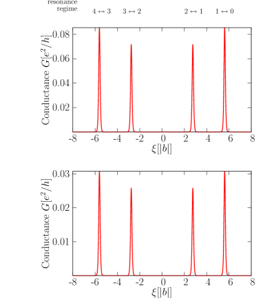
Figure 4: (Color online) Conductance at low bias for the parallel case $\Theta=0$ (top) and antiparallel case $\Theta=\pi$ (bottom). Notice the different peak heights and the mirror symmetry with respect to the half filling value $\xi=0$. The conductance in the antiparallel configuration is always smaller than in the parallel one.

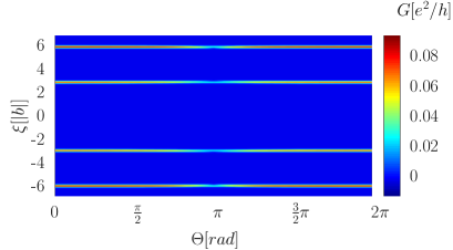
Figure 5: (Color online) Conductance as a function of the polarization angle and of the gate voltage. The minimal conductance peaks occur as expected at $\Theta=\pi$

The conductance suppression nearby $\Theta=\pi$ is clearly seen.

In the following we analyze in detail the single resonance transitions. Due to the mirror symmetry it is convenient to investigate together the resonances $N=0\leftrightarrow N=1$, $N=3\leftrightarrow N=4$ and $N=1\leftrightarrow N=2$, $N=2\leftrightarrow N=3$. We use the convention that, for a fixed resonance, the parameter $\xi=0$ when $\mu_{N+1}=0$.

IV.3.1 Resonant regimes $N=0\leftrightarrow N=1$ and $N=3\leftrightarrow N=4$

The expected mirror symmetry of $G_{01}$ and $G_{34}$ is shown in Figure 6, where the conductance peaks are plotted for different polarization angles $\Theta$ of the contacts. Notice that the analytical expressions (IV.3) (continuous lines) perfectly match the results obtained from a numerical integration of the master equation (21) with the current formula (25). We also can see that the maxima of the conductance decrease with $\Theta$ growing up to $\pi$.

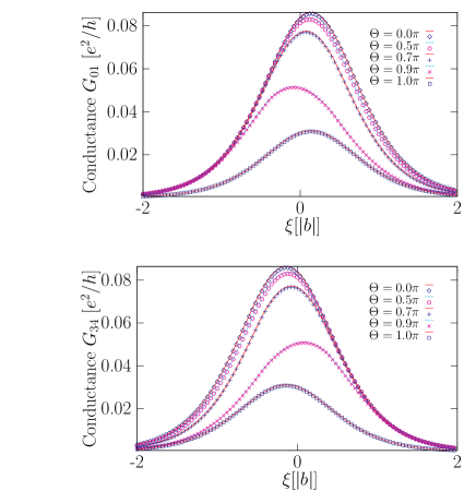
Figure 6: (Color online) The conductance $G_{01}(\xi)$ (upper figure) resp. $G_{34}(\xi))$ (lower figure) vs gate voltage for different polarization angles. The mirror symmetry of the conductance peaks for the $0\leftrightarrow 1$ and $3\leftrightarrow 4$ transitions is clearly observed. Notice the excellent agreement between the prediction of the analytical formula Eq. (IV.3) (continuous lines) and the results of a numerical integration of Eqs. (21) with (25) (symbols).

It can be shown that the peaks for $\Theta=0$ and $\Theta=\pi$ lie at the same value of $\xi$, because the effective fields $B_{i}$ exactly vanish due to trigonometrical prefactors. In other words, virtual processes captured in the effective fields $B_{i}$ do not play a role in the collinear case. For noncollinear configurations, however, the peak maxima are shifted towards the gate voltages where an odd population of the dot dominates, because there the effective exchange field can act on the accumulating spin and makes it precess, which eases tunneling out. These findings are in agreement with results obtained for a single-level quantum dot K nig03 , a metallic island Wetzels05 and carbon nanotubes Koller07 .

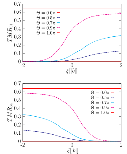
Figure 7: (Color online) Tunneling magnetoresistance (TMR) for the transitions $0\leftrightarrow 1$ (upper figure) and $3\leftrightarrow 4$ (lower figure) vs gate voltage. The TMR is always positive and is independent of gate voltage for collinear lead magnetizations only, $\Theta=0$ and $\Theta=\pi$.

To quantify the relative magnitude of the current for a given polarization angle $\Theta$ with respect to the case $\Theta=0$ we introduce the angle-dependent tunneling magnetoresistance (TMR) as

$$TMR_{N\,N+1}(\Theta,\xi)=1-\frac{G_{N,N+1}(\Theta,\xi)}{G_{N,N+1}(0,\xi)}.$$

For the transition $0\leftrightarrow 1$ it reads

$$TMR_{01}=\frac{p^{2}\sin^{2}(\frac{\Theta}{2})}{1+[B_{1}^{2}/f^{2}(-\mu_{1})\Gamma^{2}]\cos^{2}(\frac{\Theta}{2})}\;.$$ (48)

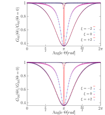
Figure 8: (Color online) $G_{01}(\Theta)/G_{01}(0)$ (upper figure) resp. $G_{34}(\Theta)/G_{34}(0)$ (lower figure) vs polarization angle. For all the three chosen values of the gate voltage the curve display an absolute minimum at $\Theta=\pi$. Notice the overall agreement of the analytical predictions (IV.3) given by the continuous curves with outcomes of a numerical solution of the master equation, Eq. (21), together with (25)(symbols).

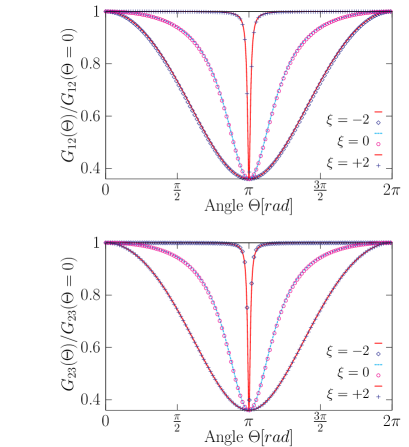
Figure 9: (Color online) $G_{12}(\Theta)/G_{12}(0)$ (upper figure) resp. $G_{23}(\Theta)/G_{23}(0)$ (lower figure) vs polarization angle. Notice the overall agreement of the analytical predictions (IV.3) and (IV.3), continuous lines, with the data (symbols) coming from a numerical solutions of the equations for the reduced density matrix.

Hence, the TMR vanishes for $\Theta=0$ and takes the constant value

$$TMR_{01}(\pi,\xi)=p^{2}$$

at $\Theta=\pi$. For the remaining polarization angles, $\Theta\neq 0$ and $\Theta\neq\pi$, the TMR is gate-voltage dependent and positive. The behavior of the TMR as a function of the gate voltage is shown in figure 7. To understand the gate voltage dependence of the TMR at noncollinear angles we have to remember that the dot is depleted with raising $\xi$. For the transition $0\leftrightarrow 1$, this means that at positive $\xi$, the dot is predominantly empty, so that an electron which enters the dot also fast leaves it. In this situation the TMR is finite and its value depends in a complicated way on the amplitude of the exchange field. At negative $\xi$, the DD is predominantly occupied with an electron which can now interact with the exchange field, which makes the spin precess and thus eases tunneling out of the dot. Consequently, $G_{NN+1}(\Theta,\xi)\approx G_{NN+1}(0,\xi)$ and the TMR vanishes. Finally, figure 8 illustrates the angular dependence of the normalized conductance for three different values of the gate voltage. We detect a common absolute minimum for the conductance at $\Theta=\pi$, i.e., transport is weakened in the antiparallel case. The width of the curves is dependent on the renormalized effective exchange $(\gamma B_{i})/(\Gamma f)$. The larger its value the narrower get the curves, because the spin precession can equilibrate the accumulated spin for all angles but $\Theta=\pi$. Notice again the equivalence of the curves belonging to $\xi=\pm 2|b|$ for the $1\leftrightarrow 2$ resonance to the curves with $\xi=\mp 2|b|$ for the $3\leftrightarrow 4$ resonance.

IV.3.2 Resonant regimes $N=1\leftrightarrow N=2$ and $N=2\leftrightarrow N=3$

For the resonant transitions $1\leftrightarrow 2$ and $2\leftrightarrow 3$ qualitatively analogous results as for the $0\leftrightarrow 1$ and $3\leftrightarrow 4$ transitions are found. Thus, exemplarily we only show the angular dependence of the normalized conductance in Fig. 9, showing the expected absolute conductance minimum at $\Theta=0$.

V Nonlinear transport

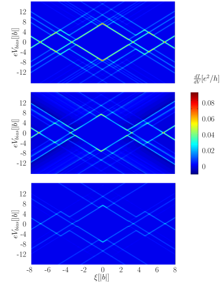
Figure 10: (Color online) Differential conductance $\frac{dI}{dV}$ for the parallel $\Theta=0$ (top), perpendicular $\Theta=\pi/2$ (middle) and antiparallel $\Theta=\pi$ (bottom) configurations. The two half diamonds and three diamonds regions correspond to bias and gate voltage values where transport is Coulomb blocked. The excitation lines, where excited states contribute to resonant transport, are clearly visible in all of the three cases. However, a negative differential conductance is observed in the perpendicular case, while some excitation lines are absent in the antiparallel configuration.

In this section we present the numerical results, deduced from the general master equation (21) combined with the current formula (25).

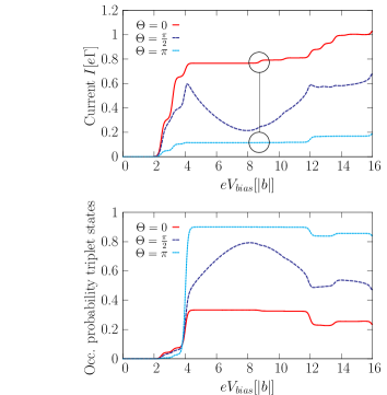
Figure 11: (Color online) Current (top) and triplet occupation (bottom) for the two collinear ($\Theta=0$,$\Theta=\pi$) cases and the perpendicular case ($\Theta=\frac{\pi}{2}$) at a fixed gate voltage $\xi=4|b|$. Notice the occurrence of a pronounced negative differential conductance feature for perpendicular polarization $\Theta=\pi/2$.

We show the differential conductance $\frac{dI}{dV}(\xi,V_{bias})$ for the three distinct angles $\Theta=0$, $\Theta=\frac{\pi}{2}$ and $\Theta=\pi$, see figure 10, top, middle and bottom, respectively. The results confirm the electron-hole-symmetry and the symmetry upon bias voltage inversion $I(\xi,V_{bias})=-I(\xi,-V_{bias})$. In all of the three cases we can nicely see the expected three closed and the two half-open diamonds, where the current is blocked and the electronic number of the double-dot-system stays constant. At higher bias voltages the contribution of excited states is manifested in the appearance of several excitation lines. One clearly sees that transition lines present in the parallel case are absent in the antiparallel case. Moreover, in the case of noncollinear polarization, $\Theta=\pi/2$, negative differential conductance (NDC) is observed.
In the following, we want not only to explain the origin of these two features, but alongside also give another example for spin-blockade effects, which play a decisive role in the DD physics.
As a starting point, we plot in figure 11 (top) the current through the system for the three different angles $\Theta=\left\{0,\frac{\pi}{2},\pi\right\}$ at a fixed gate voltage $\xi=4|b|$ and positive bias voltages. We recognize, that for $eV_{Bias}<2.4|b|\,$ the current is Coulomb-blocked in all of the three cases. In this configuration exactly one electron stays in the double-dot. From about $eV_{Bias}\geq 2.4|b|\,$ the channel where the groundstate energies $\mu_{1}$ and $\mu_{2}$ are degenerate opens ($|1e\sigma\rangle\leftrightarrow|2\rangle$ transition) and current begins to flow. With increasing bias more and more transport channels become energetically favorable. In particular, for all the polarization angles $\Theta$ we observe two consecutive steps corresponding to the transitions $|0\rangle\leftrightarrow|1e\sigma\rangle$ and $|1e\sigma\rangle\leftrightarrow|2^{\prime}\rangle$. The latter, occurring at about $eV_{bias}=4|b|$, involves the excited two-particle triplet states $|2^{\prime}(S_{z})\rangle$.
The next excitation step, indicated with a circle in Fig. 11 (top), belongs to the transition $|1o\sigma\rangle\leftrightarrow|2^{\prime\prime}\rangle$. The associated line is missing for the antiparallel configuration, as well as the lines corresponding to $|1o\sigma\rangle\leftrightarrow|2^{\prime\prime\prime}\rangle$; $|1e\sigma\rangle\leftrightarrow|2^{\prime\prime}\rangle$; $|2\rangle\leftrightarrow|3o\sigma\rangle$; $|1e\sigma\rangle\leftrightarrow|2^{\prime\prime\prime}\rangle$. Crucially, in all of these transitions a two-particle state with total spin zero is involved. In order to explain the absence of these lines, let us e.g. focus on the first missing step corresponding to the $|1o\sigma\rangle\leftrightarrow|2^{\prime\prime}\rangle$ resonance. In the parallel case (say both contacts polarized spin-up) there is always an open channel corresponding to the situation in which the spin in the DD is antiparallel to that in the leads (i.e. $|1o-\rangle$). In the antiparallel case (say source polarized spin-up, drain polarized spin-down) originally a spin-down might be present in the dot. An electron which enters the DD from the source must then be spin-up (in order to form the state $|2^{\prime\prime}\rangle$), but as the drain is down-polarized, it will be the spin-down electron which leaves the DD, which corresponds to a spin flip. Now the presence of a spin-up electron in the DD prevents a majority (another spin-up) electron from the source to enter the DD, such that we end up in a blocking state. The transition is hence forbidden.

A similar, yet different spin-blockade effect determines the occupation probabilities for the triplet state, Fig. 11 (bottom). Naturally, for all angles the probability to be in the triplet state increases above the resonance at $eV_{bias}=4|b|$, but interestingly, such probability is largest in the antiparallel case. This is due to the fact that a majority spin in the parallel configuration (spin-up) can be easily transmitted through the DD via the triplet states $|2^{\prime}(1)\rangle$ or $|2^{\prime}(0)\rangle$. In the antiparallel case, however, a blocking state establishes (say again source polarized spin-up, drain polarized spin-down). Let initially a spin-down electron be present on the DD. From the source electrode, most likely a majority electron polarized spin-up electron will enter the dot. Now, just as in the previous case, the consecutive tunneling event will cause a spin flip in the DD, because the spin-down electron (majority electron of the drain) will leave the dot. So the DD is finally in a spin-up state, and once the next majority spin-up electron from the source enters, the DD ends up in the triplet state $|2^{\prime}(+1)\rangle$ and will remain there for a long time due to the fact that the majority spins in the drain are down-polarized. Hence the triplet state $|2^{\prime}(+1)\rangle$ acts as a trapping state.

Notice that the two distinct spin-blockade effects are different from the Pauli spin-blockade discussed in the DD literature Ono02 ; Liu05 ; Johnson05 ; Fransson06 . Moreover, the second effect, relying on the existence of degenerate triplet states, is also different from the spin-blockade found in Ref. K nig03 for a single level quantum dot.

Finally, let us turn to the negative differential conductance, which occurs for noncollinearly polarized leads (see the dashed blue lines in figure 11), and which we find to become more evident for higher polarizations (not shown). Neglecting the exchange field, we would just expect the magnitude of the current for the noncollinear polarizations to lie somewhere in between the values for the parallel and the antiparallel current, because the noncollinear polarization could in principle be rewritten as a linear combination of the parallel and the antiparallel configuration. Now the effect of the exchange is to cause precession and therewith equilibration of the accumulating spin, which corresponds to shifting the balance in favor of the parallel configuration, i.e. enhancing the current. The decisive point is that the exchange field is not only gate, but also bias voltage dependent and reaches a minimum around $eV_{Bias}\approx 8|b|$. This explains the decreasing of the current up to this point. Afterwards the influence of the spin precession regains weight. The same consideration applies for the other NDC regions observed in Fig. 10, e.g. in the gate voltage region $\xi\approx 2|b|$ involving the $N=0\leftrightarrow N=1$ transition, as described in Ref. K nig03 .

VI The effects of an external magnetic field

In this section we wish to discuss the qualitative changes brought by an external magnetic field applied to the DD. Specifically, the magnetic field is assumed to be parallel to the magnetization direction of the drain. For simplicity we focus on the experimental standard case of parallel and antiparallel lead polarization and of low bias voltages. Then, the magnetic field causes an energy shift $\mp E_{Zeeman}$ depending on whether the electron spin is parallel or antiparallel, respectively, to it. For collinear polarization angles the principal part contributions vanish, and the equations for the RDM are easily obtained. We report exemplarily results for the transitions $0\leftrightarrow 1$ and $1\leftrightarrow 2$.

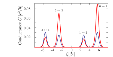
Figure 12: (Color online) Conductance vs gate voltage for parallel (continuous line) and antiparallel (dashed lines) contact configuration and Zeeman splitting $E_{Zeeman}=0.05|b|$. The magnetic field breaks the mirror symmetry with respect to the gate voltage in the parallel configuration.

Let us then consider the parameter regime nearby the $0\leftrightarrow 1$ resonance, and setup a system of three equations with three unknown variables $W_{0},W_{1\uparrow}$ and $W_{1\downarrow}$. The first equation corresponds to the normalization condition $W_{1\uparrow}+W_{1\downarrow}+W_{0}=1$. The remaining equations are the equations of motion for $W_{1\uparrow/\downarrow}$ which can be written as

$$\dot{W}_{1\uparrow} = -\frac{\pi}{\hbar}\sum_{\alpha=s,d}|t_{\alpha}|^{2}\left[F^{-}_{\alpha\uparrow}(\mu_{1\uparrow})W_{1\uparrow}\right.$$ (49)

$$- \left.F^{+}_{\alpha\uparrow}(\mu_{1\uparrow})W_{0}\right],$$

$$\dot{W}_{1\downarrow} = -\frac{\pi}{\hbar}\sum_{\alpha=s,d}|t^{\alpha}|^{2}\left[F^{-}_{\alpha\downarrow}(\mu_{1\downarrow})W_{1\downarrow}\right.$$ (50)

$$- \left.F^{+}_{\alpha\downarrow}(\mu_{1\downarrow})W_{0}\right],$$

where

$$\mu_{1\uparrow/\downarrow}=\mu_{1}\mp E_{Zeeman},$$ (51)

and $F^{\pm}_{\alpha\sigma_{\odot}}(E)=D_{\alpha\sigma_{\odot}}f^{\pm}(E)$. For the collinear case is $D_{\alpha\sigma_{\odot}}=D_{\alpha\pm_{\alpha}}$ if $\sigma_{\odot}=\uparrow/\downarrow$ in the parallel case. On the other hand $D_{s\sigma_{\odot}}=D_{s\mp_{s}}$ and $D_{d\sigma_{\odot}}=D_{d\pm_{d}}$, if $\sigma_{\odot}=\uparrow/\downarrow$, in the antiparallel case.

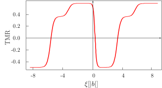
Figure 13: (Color online) Tunneling magnetoresistance (TMR) vs gate voltage in the presence of an external magnetic field. In contrast to the zero field case, the TMR can become negative in the vicinity of the $2\leftrightarrow 3$ and $3\leftrightarrow 4$ resonances.

Upon considering symmetric contacts ($t_{1}=t_{2}=t$, $D_{1}=D_{2}=D$) we find in the parallel case

$$G_{01}(\Theta=0)=\frac{\Gamma e^{2}}{8\beta}f(-\mu_{1\uparrow})f(-\mu_{1\downarrow})$$

$$\times \frac{p\left(f(\mu_{1\uparrow})-f(\mu_{1\downarrow})\right)+f(\mu_{1\uparrow})+f(\mu_{1\downarrow})}{f(-\mu_{1\uparrow})f(\mu_{1\downarrow})+f(-\mu_{1\uparrow})f(-\mu_{1\downarrow})+f(\mu_{1\uparrow})f(-\mu_{1\downarrow})}.$$

For the antiparallel case we obtain

$$G_{01}(\Theta=\pi)=G_{01}(\Theta=0)$$

$$\times\frac{1-p^{2}\left(f(\mu_{1\uparrow})+f(\mu_{1\downarrow})\right)}{p\;[f(\mu_{1\uparrow})-f(\mu_{1\downarrow})]+f(\mu_{1\uparrow})+f(\mu_{1\downarrow})}.$$

Analogously we find for the $1\leftrightarrow 2$ transition

$$G_{12}(\Theta=0)=\frac{\Gamma e^{2}k_{+}^{2}}{2\beta}f(\mu_{2\uparrow})f(\mu_{2\downarrow})$$

$$\times \frac{p\left(f(-\mu_{2\downarrow})-f(-\mu_{2\uparrow})\right)+f(-\mu_{2\uparrow})+f(-\mu_{2\downarrow})}{f(-\mu_{2\uparrow})f(\mu_{2\downarrow})+f(-\mu_{2\uparrow})f(-\mu_{2\downarrow})+f(\mu_{2\uparrow})f(-\mu_{2\downarrow})},$$

$$G_{12}(\Theta=\pi)=G_{12}(\Theta=0)$$

$$\times \frac{1-p^{2}(f(-\mu_{2\uparrow})+f(-\mu_{2\downarrow}))}{p\;,[f(-\mu_{2\downarrow})-f(-\mu_{2\uparrow})]+f(-\mu_{2\uparrow})+f(-\mu_{2\downarrow})}.$$

The remaining resonances are calculated analogously. Figure 12 shows the four conductance resonances for the parallel and antiparallel configurations. Strikingly, the applied magnetic field breaks the symmetry between the tunneling regimes $0\leftrightarrow 1$ and $3\leftrightarrow 4$, as well as between the resonances $1\leftrightarrow 2$ and $2\leftrightarrow 3$ in case of parallel contact polarizations. The reason for this behavior is the following: In the low bias regime transitions between groundstates dominate transport. In particular, the magnetic field removes the spin degeneracy of the states $|1e\sigma\rangle$ and of the states $|3o\sigma\rangle$, such that states with spin aligned to the external magnetic field are energetically favored. Therefore, the transport electron in the tunneling regime $0\leftrightarrow 1$ is a majority spin carrier. For the case $3\leftrightarrow 4$, however, two of the three electrons of the groundstate $|3o+\rangle$ have spin-up, such that the fourth electron which can be added to the DD has to be a minority spin carrier. Therefore, the conductance gets diminished with respect to the $0\leftrightarrow 1$ transition, and the mirror symmetry present in the zero field case is broken. Analogously the broken symmetry in the case of the transitions $1\leftrightarrow 2$ and $2\leftrightarrow 3$ can be understood. Correspondingly, the TMR can become negative for values of the gate voltages around the $2\leftrightarrow 3$ and $3\leftrightarrow 4$ resonances. We observe that a negative TMR has recently been predicted in Cottet06 for the case of a single impurity Anderson model with orbital and spin degeneracy. In that work a negative TMR arises due to the assumption that multiple reflections at the interface cause spin-dependent energy shifts. In our approach, however, where the contribution from the reflection Hamiltonian is treated to the lowest order, see (19), such spin-dependent energies are originating from the magnetic field-induced Zeeman splitting.

VII Conclusions

In summary we have evaluated linear and nonlinear transport through a double quantum dot (DD) coupled to polarized leads with arbitrary polarization directions. Due to strong Coulomb interactions the DD operates as a single-electron transistor, a F-SET, at low enough temperatures. A detailed analysis of the current-voltage characteristics of the DD, and comparison with results of previous studies on other F-SET systems with noncollinear (a single level quantum dot K nig03 , a metallic island Wetzels05 , a carbon nanotube Koller07 ), bring us to the identification of universal behaviors of a F-SET, i.e., a behavior shared by any of those F-SETs, independent of the specific kind of conductor is considered as the central system, as well as system-specific features.
Universal is the presence of an interfacial exchange field together with an interaction-induced one, present for noncollinear polarization only. These exchange fields cause a precession of the accumulated spin on the dot and therewith ease the tunneling out. This effect has various implications. It determines e.g. the gate and angular dependence, as well as the height of single conductance peaks and can yield negative differential conductance features. Another universal feature is the occurrence of a negative tunneling magnetoresistance - even in the weak tunneling limit - if an external magnetic field is applied.
Specific to the DD system are the following features: In the low bias regime, the problem can be solved analytically and for the tunneling regimes $0\leftrightarrow 1$ and $1\leftrightarrow 2$, respectively $2\leftrightarrow 3$ and $3\leftrightarrow 4$, the system behaves equivalent to a single level quantum dot, where the Coulomb blockade peaks are found to be mirror-symmetric with respect to the charge neutrality point. This mirror symmetry reflects the electron-hole-symmetries of a system and is therefore typical for the DD, as well as the ratio of the peak heights. An external magnetic field lifts this symmetry and can cause a negative tunneling magnetoresistance. In the nonlinear bias regime, the presence of various excited states gives rise to interesting DD specific features. For example, a suppression of several excitation lines for an antiparallel lead configuration originates from a spin-blockade effect. It occurs because a trapping state is formed whenever a transition involves a two-electron state with total spin zero. A second spin-blockade effect we described involves the two-electron triplet state. The common mechanism of these two spin-blockades is the following: in both cases, a tunneling event can only occur if initially the dot is populated with an unpaired electron possessing the majority spin of the drain. The second step is that a majority electron of the source will enter, forming a spin-zero state. Then the first electron can leave the dot, causing a spin-flip. If the triplet state is involved, the dot will be left in a trapping state once a second majority electron from the source enters. Otherwise, we are directly in a blocking state. Finally, for noncollinear lead polarizations, negative differential conductance can be observed.
All in all, due to their universality and the multiplicity of their properties, F-SET based on DD systems seem good candidates for future magneto-electronic devices.

Appendix A Matrix elements of the dot operators

The following tables show all the possible matrix-elements $\langle{N-1}|d_{\alpha\sigma_{\odot}}|N\rangle$ and $\langle{N}|d^{\dagger}_{\alpha\sigma_{\odot}}|{N-1}\rangle$ with $\alpha=\left\{1,2\right\}$ and $\sigma_{\odot}=\left\{\uparrow,\downarrow\right\}$ which occur in the master equations (B) and (B). Notice that we only need to illustrate either the matrix elements $\langle{N-1}|d_{\alpha\sigma_{\odot}}|N\rangle$ or $\langle{N}|d^{\dagger}_{\alpha\sigma_{\odot}}|{N-1}\rangle$, because they are complex conjugated to each other.

		$0\leftrightarrow 1$
	$|{1e\uparrow}\rangle$	$|{1e\downarrow}\rangle$	$|{1o\uparrow}\rangle$	$|{1o\downarrow}\rangle$
$d_{1\uparrow}:\langle 0\lvert$	$\frac{1}{\sqrt{2}}$	$0$	$\frac{1}{\sqrt{2}}$	0
$d_{1\downarrow}:\langle 0\lvert$	0	$\frac{1}{\sqrt{2}}$	0	$\frac{1}{\sqrt{2}}$
$d_{2\uparrow}:\langle 0\lvert$	$\frac{1}{\sqrt{2}}$	0	$-\frac{1}{\sqrt{2}}$	0
$d_{2\downarrow}:\langle 0\lvert$	0	$\frac{1}{\sqrt{2}}$	0	$-\frac{1}{\sqrt{2}}$

Table 2: Matrix elements for the transition $N=0\leftrightarrow N=1$ induced by the operators $d_{\alpha\uparrow}$ and $d_{\alpha\downarrow}$, $\alpha=1,2$.

			$1\leftrightarrow 2$
		$|{1e\uparrow}\rangle$	$|{1e\downarrow}\rangle$	$|{1o\uparrow}\rangle$	$|{1o\downarrow}\rangle$
	$\langle 2g\lvert$	$0$	$\frac{\alpha_{0}+\beta_{0}}{2}$	$0$	$\frac{-\alpha_{0}+\beta_{0}}{2}$
	$\langle 2^{\prime}(+1)\lvert$	$\frac{1}{\sqrt{2}}$	$0$	$-\frac{1}{\sqrt{2}}$	$0$
$d^{\dagger}_{1\uparrow}:$	$\langle 2^{\prime}(0)\lvert$	$0$	$\frac{1}{2}$	$0$	$-\frac{1}{2}$
	$\langle 2^{\prime}(-1)\lvert$	$0$	$0$	$0$	$0$
	$\langle 2^{\prime\prime}\lvert$	$0$	$\frac{1}{2}$	$0$	$\frac{1}{2}$
	$\langle 2^{\prime\prime\prime}\lvert$	$0$	$\frac{-\alpha_{0}+\beta_{0}}{2}$	$0$	$\frac{-\alpha_{0}-\beta_{0}}{2}$
	$\langle 2g\lvert$	$\frac{-\alpha_{0}-\beta_{0}}{2}$	$0$	$\frac{\alpha_{0}-\beta_{0}}{2}$	$0$
	$\langle 2^{\prime}(+1)\lvert$	$0$	$0$	$0$	$0$
$d^{\dagger}_{1\downarrow}:$	$\langle 2^{\prime}(0)\lvert$	$\frac{1}{2}$	$0$	$-\frac{1}{2}$	$0$
	$\langle 2^{\prime}(-1)\lvert$	$0$	$\frac{1}{\sqrt{2}}$	$0$	$-\frac{1}{\sqrt{2}}$
	$\langle 2^{\prime\prime}\lvert$	$-\frac{1}{2}$	$0$	$-\frac{1}{2}$	$0$
	$\langle 2^{\prime\prime\prime}\lvert$	$\frac{\alpha_{0}-\beta_{0}}{2}$	$0$	$\frac{\alpha_{0}+\beta_{0}}{2}$	$0$
	$\langle 2g\lvert$	$0$	$\frac{\alpha_{0}+\beta_{0}}{2}$	$0$	$\frac{\alpha_{0}-\beta_{0}}{2}$
	$\langle 2^{\prime}(+1)\lvert$	$-\frac{1}{\sqrt{2}}$	$0$	$-\frac{1}{\sqrt{2}}$	$0$
$d^{\dagger}_{2\uparrow}:$	$\langle 2^{\prime}(0)\lvert$	$0$	$-\frac{1}{2}$	$0$	$-\frac{1}{2}$
	$\langle 2^{\prime}(-1)\lvert$	$0$	$0$	$0$	$0$
	$\langle 2^{\prime\prime}\lvert$	$0$	$-\frac{1}{2}$	$0$	$\frac{1}{2}$
	$\langle 2^{\prime\prime\prime}\lvert$	$0$	$\frac{-\alpha_{0}+\beta_{0}}{2}$	$0$	$\frac{\alpha_{0}+\beta_{0}}{2}$
	$\langle 2g\lvert$	$\frac{-\alpha_{0}-\beta_{0}}{2}$	$0$	$\frac{-\alpha_{0}+\beta_{0}}{2}$	$0$
	$\langle 2^{\prime}(+1)\lvert$	$0$	$0$	$0$	$0$
$d^{\dagger}_{2\downarrow}:$	$\langle 2^{\prime}(0)\lvert$	$-\frac{1}{2}$	$0$	$-\frac{1}{2}$	$0$
	$\langle 2^{\prime}(-1)\lvert$	$0$	$-\frac{1}{\sqrt{2}}$	$0$	$-\frac{1}{\sqrt{2}}$
	$\langle 2^{\prime\prime}\lvert$	$\frac{1}{2}$	$0$	$-\frac{1}{2}$	$0$
	$\langle 2^{\prime\prime\prime}\lvert$	$\frac{\alpha_{0}-\beta_{0}}{2}$	$0$	$\frac{-\alpha_{0}-\beta_{0}}{2}$	$0$

Table 3: Matrix elements for the transition $N=1\leftrightarrow N=2$ induced by $d^{\dagger}_{\alpha\uparrow}$ and $d^{\dagger}_{\alpha\downarrow}$, $\alpha=1,2$. The notation $|2^{\prime}(s_{z})\rangle$, with $s_{z}=0,\pm 1$, specifies which one of the triplet elements is addressed.

			$2\leftrightarrow 3$
		$|{3o\uparrow}\rangle$	$|{3o\downarrow}\rangle$	$|{3e\uparrow}\rangle$	$|{3e\downarrow}\rangle$
	$\langle 2g\lvert$	$\frac{\alpha_{0}+\beta_{0}}{2}$	$0$	$\frac{\alpha_{0}-\beta_{0}}{2}$	$0$
	$\langle 2^{\prime}(+1)\lvert$	$0$	$0$	$0$	$0$
$d_{1\uparrow}:$	$\langle 2^{\prime}(0)\lvert$	$-\frac{1}{2}$	$0$	$-\frac{1}{2}$	$0$
	$\langle 2^{\prime}(-1)\lvert$	$0$	$\frac{1}{\sqrt{2}}$	$0$	$\frac{1}{\sqrt{2}}$
	$\langle 2^{\prime\prime}\lvert$	$-\frac{1}{2}$	$0$	$\frac{1}{2}$	$0$
	$\langle 2^{\prime\prime\prime}\lvert$	$\frac{-\alpha_{0}+\beta_{0}}{2}$	$0$	$\frac{\alpha_{0}+\beta_{0}}{2}$	$0$
	$\langle 2g\lvert$	$0$	$\frac{-\alpha_{0}-\beta_{0}}{2}$	$0$	$\frac{-\alpha_{0}+\beta_{0}}{2}$
	$\langle 2^{\prime}(+1)\lvert$	$\frac{1}{\sqrt{2}}$	$0$	$\frac{1}{\sqrt{2}}$	$0$
$d_{1\downarrow}:$	$\langle 2^{\prime}(0)\lvert$	$0$	$-\frac{1}{2}$	$0$	$-\frac{1}{2}$
	$\langle 2^{\prime}(-1)\lvert$	$0$	$0$	$0$	$0$
	$\langle 2^{\prime\prime}\lvert$	$0$	$\frac{1}{2}$	$0$	$-\frac{1}{2}$
	$\langle 2^{\prime\prime\prime}\lvert$	$0$	$\frac{\alpha_{0}-\beta_{0}}{2}$	$0$	$\frac{-\alpha_{0}-\beta_{0}}{2}$
	$\langle 2g\lvert$	$\frac{-\alpha_{0}-\beta_{0}}{2}$	$0$	$\frac{\alpha_{0}-\beta_{0}}{2}$	$0$
	$\langle 2^{\prime}(+1)\lvert$	$0$	$0$	$0$	$0$
$d_{2\uparrow}:$	$\langle 2^{\prime}(0)\lvert$	$-\frac{1}{2}$	$0$	$\frac{1}{2}$	$0$
	$\langle 2^{\prime}(-1)\lvert$	$0$	$\frac{1}{\sqrt{2}}$	$0$	$-\frac{1}{\sqrt{2}}$
	$\langle 2^{\prime\prime}\lvert$	$-\frac{1}{2}$	$0$	$-\frac{1}{2}$	$0$
	$\langle 2^{\prime\prime\prime}\lvert$	$\frac{\alpha_{0}-\beta_{0}}{2}$	$0$	$\frac{\alpha_{0}+\beta_{0}}{2}$	$0$
	$\langle 2g\lvert$	$0$	$\frac{\alpha_{0}+\beta_{0}}{2}$	$0$	$\frac{-\alpha_{0}+\beta_{0}}{2}$
	$\langle 2^{\prime}(+1)\lvert$	$\frac{1}{\sqrt{2}}$	$0$	$-\frac{1}{\sqrt{2}}$	$0$
$d_{2\downarrow}:$	$\langle 2^{\prime}(0)\lvert$	$0$	$-\frac{1}{2}$	$0$	$\frac{1}{2}$
	$\langle 2^{\prime}(-1)\lvert$	$0$	0	$0$	0
	$\langle 2^{\prime\prime}\lvert$	$0$	$\frac{1}{2}$	$0$	$\frac{1}{2}$
	$\langle 2^{\prime\prime\prime}\lvert$	$0$	$\frac{-\alpha_{0}+\beta_{0}}{2}$	$0$	$\frac{-\alpha_{0}-\beta_{0}}{2}$

Table 4: Matrix elements for the transition $N=2\leftrightarrow N=3$ governed by $d_{\alpha\uparrow}$ and $d_{\alpha\downarrow}$, $\alpha=1,2$.

		$3\leftrightarrow 4$
	$|{3o\uparrow}\rangle$	$|{3o\downarrow}\rangle$	$|{3e\uparrow}\rangle$	$|{3e\downarrow}\rangle$
$d^{\dagger}_{1\uparrow}:\langle 2,2\lvert$	$0$	$\frac{1}{\sqrt{2}}$	$0$	$-\frac{1}{\sqrt{2}}$
$d^{\dagger}_{1\downarrow}:\langle 2,2\lvert$	$\frac{1}{\sqrt{2}}$	$0$	$-\frac{1}{\sqrt{2}}$	$0$
$d^{\dagger}_{2\uparrow}:\langle 2,2\lvert$	$0$	$-\frac{1}{\sqrt{2}}$	$0$	$-\frac{1}{\sqrt{2}}$
$d^{\dagger}_{2\downarrow}:\langle 2,2\lvert$	$-\frac{1}{\sqrt{2}}$	$0$	$-\frac{1}{\sqrt{2}}$	$0$

Table 5: Matrix elements for the transition $N=3\leftrightarrow N=4$ induced by the operators $d^{\dagger}_{\alpha\uparrow}$ and $d^{\dagger}_{\alpha\downarrow}$, $\alpha=1,2$.

Appendix B The master equation for the RDM in the linear regime

We report here explicitly the coupled equations of motion for the elements $\dot{{\rho}}_{nm}^{(N)}(t)$ and $\dot{{\rho}}_{nm}^{(N+1)}(t)$ of the RDM to be solved in the low bias regime. They are obtained from the generalized master equation (21) upon observing that i) in the linear regime terms that couple states with particle numbers unlike $N$ and $N+1$ can be neglected; ii) we can reduce the sum over $h$ and $h^{\prime}$ and over $l,l^{\prime}$ only to energy ground states. In the remaining not energy conserving terms the sum has to go also over excited states. With $\mu_{N+1}:=E^{(0)}_{N+1}-E^{(0)}_{N}$ being the chemical potential we finally arrive at the two master equations

$$\dot{{\rho}}_{nm}^{(N)}(t) =$$

$$-\frac{\pi}{\hbar}\sum_{\alpha=s,d}|{t^{\alpha}}|^{2}\sum_{\sigma_{\odot},\sigma_{\odot}^{\prime}}\quad\left\{\sum_{l\in{|{N-1}\rangle}},\quad\sum_{j\in|E^{(0)}_{N},N\rangle},\quad\sum_{h,h^{\prime}\in{|{E^{(0)}_{N+1},N+1}\rangle}},\quad\sum_{\widehat{h}\in{|{N+1}\rangle}}\right\}\left\{\right.$$

$$\qquad+\Phi_{\alpha\sigma_{\odot}\sigma_{\odot}^{\prime}}F^{+}_{\alpha\sigma_{\odot}\sigma_{\odot}^{\prime}}(\mu_{N+1})\quad\big{(}d_{\alpha\sigma_{\odot}}\big{)}_{nh}\quad\big{(}d^{\dagger}_{\alpha\sigma_{\odot}^{\prime}}\big{)}_{hj}\quad{\rho}_{jm}^{(N)}(t)$$

$$\qquad+\Phi_{\alpha\sigma_{\odot}\sigma_{\odot}^{\prime}}\frac{i}{\pi}P^{+}_{\alpha\sigma_{\odot}\sigma_{\odot}^{\prime}}(\varepsilon_{\widehat{h}}-\varepsilon_{j})\quad\big{(}d_{\alpha\sigma_{\odot}}\big{)}_{n\widehat{h}}\quad\big{(}d^{\dagger}_{\alpha\sigma_{\odot}^{\prime}}\big{)}_{\widehat{h}j}\quad{\rho}_{jm}^{(N)}(t)$$

$$\qquad-\Phi^{\ast}_{\alpha\sigma_{\odot}\sigma_{\odot}^{\prime}}\frac{i}{\pi}\left[P^{-}_{\alpha\sigma_{\odot}\sigma_{\odot}^{\prime}}(\varepsilon_{j}-\varepsilon_{l})+R_{\alpha\sigma_{\odot}\sigma^{\prime}_{\odot}}\right]\big{(}d^{\dagger}_{\alpha\sigma_{\odot}}\big{)}_{nl}\big{(}d_{\alpha\sigma_{\odot}^{\prime}}\big{)}_{lj}{\rho}_{jm}^{(N)}(t)$$

$$\qquad+\Phi_{\alpha\sigma_{\odot}\sigma_{\odot}^{\prime}}F^{+}_{\alpha\sigma_{\odot}\sigma_{\odot}^{\prime}}(\mu_{N+1})\quad{\rho}_{nj}^{(N)}(t)\quad\big{(}d_{\alpha\sigma_{\odot}}\big{)}_{jh}\quad\big{(}d^{\dagger}_{\alpha\sigma_{\odot}^{\prime}}\big{)}_{hm}$$

$$\qquad-\Phi_{\alpha\sigma_{\odot}\sigma_{\odot}^{\prime}}\frac{i}{\pi}P^{+}_{\alpha\sigma_{\odot}\sigma_{\odot}^{\prime}}(\varepsilon_{\widehat{h}}-\varepsilon_{j})\quad{\rho}_{nj}^{(N)}(t)\quad\big{(}d_{\alpha\sigma_{\odot}}\big{)}_{j\widehat{h}}\quad\big{(}d^{\dagger}_{\alpha\sigma_{\odot}^{\prime}}\big{)}_{\widehat{h}m}$$

$$\qquad+\Phi^{\ast}_{\alpha\sigma_{\odot}\sigma_{\odot}^{\prime}}\frac{i}{\pi}\left[P^{-}_{\alpha\sigma_{\odot}\sigma_{\odot}^{\prime}}(\varepsilon_{j}-\varepsilon_{l})+R_{\alpha\sigma_{\odot}\sigma^{\prime}_{\odot}}\right]{\rho}_{nj}^{(N)}(t)\big{(}d^{\dagger}_{\alpha\sigma_{\odot}}\big{)}_{jl}\big{(}d_{\alpha\sigma_{\odot}^{\prime}}\big{)}_{lm}$$

$$\qquad-2\Phi_{\alpha\sigma_{\odot}\sigma_{\odot}^{\prime}}F^{-}_{\alpha\sigma_{\odot}\sigma_{\odot}^{\prime}}(\mu_{N+1})\quad\big{(}d_{\alpha\sigma_{\odot}}\big{)}_{nh^{\prime}}\quad{\rho}_{h^{\prime}h}^{(N+1)}(t)\quad\big{(}d^{\dagger}_{\alpha\sigma_{\odot}^{\prime}}\big{)}_{hm}\left.\right\},$$

$$\dot{\rho}_{nm}^{(N+1)}(t) =$$

$$-\frac{\pi}{\hbar}\sum_{\alpha=s,d}|{t^{\alpha}}|^{2}\sum_{\sigma_{\odot},\sigma_{\odot}^{\prime}}\quad\left\{\sum_{\widehat{l}\in{|{E_{N},N}\rangle}},\quad\sum_{l,l^{\prime}\in{|{E^{(0)}_{N},N}\rangle}},\quad\sum_{j\in|{E^{(0)}_{N+1},N+1}\rangle},\quad\sum_{h\in{|{E_{N+2},N+2}\rangle}}\right\}\left\{\right.$$

$$\qquad+\Phi_{\alpha\sigma_{\odot}\sigma_{\odot}^{\prime}}\frac{i}{\pi}P^{+}_{\alpha\sigma_{\odot}\sigma_{\odot}^{\prime}}(\varepsilon_{h}-\varepsilon_{j})\quad\big{(}d_{\alpha\sigma_{\odot}}\big{)}_{nh}\quad\big{(}d^{\dagger}_{\alpha\sigma_{\odot}^{\prime}}\big{)}_{hj}\quad{\rho}_{jm}^{(N+1)}(t)$$

$$\qquad+\Phi^{\ast}_{\alpha\sigma_{\odot}\sigma_{\odot}^{\prime}}F^{-}_{\alpha\sigma_{\odot}\sigma_{\odot}^{\prime}}(\mu_{N+1})\big{(}d^{\dagger}_{\alpha\sigma_{\odot}}\big{)}_{nl}\big{(}d_{\alpha\sigma_{\odot}^{\prime}}\big{)}_{lj}{\rho}_{jm}^{(N+1)}(t)$$

$$\qquad-\Phi^{\ast}_{\alpha\sigma_{\odot}\sigma_{\odot}^{\prime}}\frac{i}{\pi}\left[P^{-}_{\alpha\sigma_{\odot}\sigma_{\odot}^{\prime}}(\varepsilon_{j}-\varepsilon_{\widehat{l}})+R_{\alpha\sigma_{\odot}\sigma^{\prime}_{\odot}}\right]\big{(}d^{\dagger}_{\alpha\sigma_{\odot}}\big{)}_{n\widehat{l}}\big{(}d_{\alpha\sigma_{\odot}^{\prime}}\big{)}_{\widehat{l}j}{\rho}_{jm}^{(N+1)}(t)$$

$$\qquad-\Phi_{\alpha\sigma_{\odot}\sigma_{\odot}^{\prime}}\frac{i}{\pi}P^{+}_{\alpha\sigma_{\odot}\sigma_{\odot}^{\prime}}(\varepsilon_{h}-\varepsilon_{j})\quad{\rho}_{nj}^{(N+1)}(t)\quad\big{(}d_{\alpha\sigma_{\odot}}\big{)}_{jh}\quad\big{(}d^{\dagger}_{\alpha\sigma_{\odot}^{\prime}}\big{)}_{hm}$$

$$\qquad+\Phi^{\ast}_{\alpha\sigma_{\odot}\sigma_{\odot}^{\prime}}\left[F^{-}_{\alpha\sigma_{\odot}\sigma_{\odot}^{\prime}}(\mu_{N+1})\right]{\rho}_{nj}^{(N+1)}(t)\big{(}d^{\dagger}_{\alpha\sigma_{\odot}}\big{)}_{j\widehat{l}}\big{(}d_{\alpha\sigma_{\odot}^{\prime}}\big{)}_{\widehat{l}m}$$

$$\qquad+\Phi^{\ast}_{\alpha\sigma_{\odot}\sigma_{\odot}^{\prime}}\frac{i}{\pi}\left[P^{-}_{\alpha\sigma_{\odot}\sigma_{\odot}^{\prime}}(\varepsilon_{j}-\varepsilon_{\widehat{l}})+R_{\alpha\sigma_{\odot}\sigma^{\prime}_{\odot}}\right]{\rho}_{nj}^{(N+1)}(t)\big{(}d^{\dagger}_{\alpha\sigma_{\odot}}\big{)}_{j\widehat{l}}\big{(}d_{\alpha\sigma_{\odot}^{\prime}}\big{)}_{\widehat{l}m}$$

$$\qquad-2\Phi^{\ast}_{\alpha\sigma_{\odot}\sigma_{\odot}^{\prime}}F^{+}_{\alpha\sigma_{\odot}\sigma_{\odot}^{\prime}}(\mu_{N+1})\quad\big{(}d^{\dagger}_{\alpha\sigma_{\odot}}\big{)}_{nl^{\prime}}\quad{\rho}_{l^{\prime}l}^{(N)}(t)\quad\big{(}d_{\alpha\sigma_{\odot}^{\prime}}\big{)}_{lm}\left.\right\}.$$

Notice that we kept the sums over excited states $l,\widehat{h}$ in (B) and $\widehat{l},h$ in (B) which are responsible for the virtual transitions.

References

- (1) S. Maekawa and T. Shinjo, Spin Dependent Transport in Magnetic Nanostrucures (Taylor and Francis, New York 2002).
- (2) See e.g. Focus on Spintronics in reduced dimensions, ed. by G.E.W. Bauer and L.W. Molenkamp, New J. of Phys. 9 (2007).
- (3) D. D. Awscahalom, D. Loss and N. Samarth (Springer, Berlin, 2002).
- (4) Single Charge Tunneling: Coulomb Blockade Phenomena in Nanostructures, NATO ASI Series B: Physics 294, ed. by H. Grabert and M. Devoret (Plenum, New York, 1992).
- (5) Mesoscopic Electron Transport, ed. by L. L. Sohn, L.P. Kouwenhoven and G. Sch n (Kluwer, Dordrecht, 1997).
- (6) K. Ono, H. Shimada, and Y. Ootuka, J. Phys. Soc. Jpn 66, 1261 (1997).
- (7) L. F. Schelp, A. Fert, F. Fettar, P. Holody, S. F. Lee, J. L. Maurice, F. Petroff, and A. Vaurès, Phys. Rev. B 56, R5747 (1997).
- (8) K. Yakushiji, F. Ernult, H. Imamura, K. Yamane, S. Mitani, K. Takanashi, S. Takahashi, S. Maekawa, and H. Fujimori, Nature Mat. 4, 57 (2005).
- (9) L. Y. Zhang, C. Y. Wang, Y. G. Wei, X. Y. Liu, and D. Davidović, Phys. Rev. B, 72, 155445 (2005).
- (10) A. Bernand-Mantel, P. Seneor, N. Lidgi, M. Muñoz, V. Cros, S. Fusil, K. Bouzehouane, C. Deranlot, A. Vaures, F. Petroff, and A. Fert, cond-mat/0601439.
- (11) M. Pioro-Ladrière, M. Ciorga, J. Lapointe, P. Zawadzki, M. Korkusinski, P. Hawrylak and A. Sachradja, Phys. Rev. Lett. 91, 026803 (2003).
- (12) A. N. Pasupathy, R. C. Bialczak, J. Martinek, J. E. Grose, L. A. K. Donev, P. L. McEuen, and D. C. Ralph, Science 306, 86 (2004).
- (13) S. Sahoo, T. Kontos, J. Furer, C. Hoffmann, M. Gräber, A. Cottet, and C. Schönenberger, Nature Physics 1, 99 (2005).
- (14) J. Barnaś and A. Fert, Phys. Rev. Lett. 80, 1058 (1998).
- (15) S. Takahashi and S. Maekawa, Phys. Rev. Lett. 80, 1758 (1998).
- (16) K. Majumdar and S. Hershfield, Phys. Rev. B 57, 11521 (1998).
- (17) A. N. Korotkov and V. I. Safarov, Phys. Rev. B 59, 89 (1999).
- (18) A. Brataas, Yu. V. Nazarov, J. Inoue, and G. E. W. Bauer, Eur. Phys. J. B 9, 421 (1999).
- (19) A. Brataas and X. H. Wang, Phys. Rev. B 64, 104434 (2001).
- (20) I. Weymann, J. König, J. Martinek, J. Barnaś and G. Schön, Phys. Rev. B 72, 115334 (2005).
- (21) L. Y. Gorelik, S. I. Kulinich, R. I. Shekhter, M. Jonson, and V. M. Vinokur, Phys. Rev. Lett. 95, 116806 (2005).
- (22) A. Cottet and M-S. Choi, Phys. Rev. B 74, 235316 (2006).
- (23) J. Fransson, Nanotechnology 17, 5344 (2006).
- (24) I. Weymann, Phys. Rev. B 75, 195339 (2007).
- (25) Y. Tanaka and N. Kawakami, J. Phys. Soc. Jpn, Vol. 73 No. 10, pp. 2795-2801 (2004).
- (26) L. Balents and R. Egger, Phys. Rev. B 64, 035310 (2001).
- (27) C. Bena, and L. Balents, Phys. Rev. B 65, 115108 (2002).
- (28) J. N. Pedersen, J. Q.Thomassen, and K. Flensberg, Phys. Rev. B 72, 045341 (2005).
- (29) W. Wetzels, G. E. W. Bauer, and M. Grifoni, Phys. Rev. B 72, 020407(R) (2005); Phys. Rev. B 74 224406 (2006).
- (30) N. Sergueev, Qing-feng Sun, Hong Guo, B.G. Wang and Jian Wang, Phys. Rev. B 65, 165303 (2002).
- (31) J. König and J. Martinek, Phys. Rev. Lett. 90, 166602 (2003); M. Braun, J. König, and J. Martinek, Phys. Rev. B 70, 195345 (2004); J. König, J. Martinek, J. Barnaś, and G. Schön, in CFN Lectures on Functional Nanostructures, Eds. K. Busch et al., Lecture Notes in Physics 658 (Springer), pp. 145-164, (2005).
- (32) W. Rudziński, J. Barnaś, R. Świrkowicz, and M. Wilczyński, Phys. Rev. B 71, 205307 (2005).
- (33) J. Fransson, Europhys. Lett. 70, 796 (2005).
- (34) S. Braig and P. W. Brouwer, Phys. Rev. B 71, 195324 (2005).
- (35) I. Weymann and J. Barnaś, Eur. Phys. J. B 46, 289 (2005).
- (36) H.-F. Mu, G. Su, and Q.-R. Zheng, Phys. Rev. B 73, 054414 (2006).
- (37) I. Weymann and J. Barnaś, Phys. Rev. B 75, 155308 (2007).
- (38) O. Parcollet, and X. Waintal, Phys. Rev. B 73, 144420 (2006).
- (39) S. Koller, L. Mayrhofer and M. Grifoni, New J. of Phys. 9, 348 (2007).
- (40) A. Brataas, Yu. V. Nazarov, and G. E. W. Bauer, Phys. Rev. Lett. 84, 2481 (2000); A. Brataas, Y. V. Nazarov, and G. E. W. Bauer, Eur. Phys. J. B 22, 99 (2001); A. Brataas, G. E. W. Bauer and P. J. Kelly, Phys. Rep. 427, 157 (2006).
- (41) M. D. Stiles and A. Zangwill, Phys. Rev. B 66, 014407 (2002).
- (42) A. A. Tulapurkar, Y. Suzuki, A. Fukushima, H. Kubota, H. Maehara, K. Tsunekawa, D. D. Djayaprawira, N. Watanabe, and S. Yuasa, Nature 438, 339 (2005).
- (43) A. Cottet, T. Kontos, W. Belzig, C. Schönenberger, and C. Bruder, Europhys. Lett. 74, 320 (2006).
- (44) W. G. van der Wiel, S. De Franceschi, J.M. elzerman, T. Fujisawa, S. Tarucha and L. P. Kouwenhoven, Rev. Mod. Phys. 75, 1 (2002).
- (45) M. R. Gräber, W. A. Coish, C. Hoffmann, M. Weiss, J. Furer, S. Oberholzer, D. Loss and C. Schönenberger, Phys. Rev. B 74, 075427 (2006).
- (46) D. Loss and D. P. DiVincenzo, Phys. Rev. A 57, 120 (1998).
- (47) K. Ono, D. G. Austing, Y. Tokura and S. Tarucha, Science 297, 1313 (2002).
- (48) H. W. Liu, T. Fujisawa, T. Hayashi and Y. Hirayama, Phys. Rev. B 72, 161305(R) (2005).
- (49) A. C. Johnson, J. R. Petta, C. M. Marcus, M. P. Hanson and A. C. Gossard, Phys. Rev. B 72, 165308 (2005).
- (50) J. Fransson and M. Råsander, 205333 73, (2006).
- (51) J. König, H. Schoeller and G. Schön, Phys. Rev. Lett. 76, 1715 (1996).
- (52) B. R. Bułka and T. Kostryrko, Phys. Rev. B 70, 205333 (2004).
- (53) K. Blum Density matrix theory and its applications, Plenum Press (New York 2nd ed. 1996).