Surface dissipation in nanoelectromechanical systems: Unified description with the Standard Tunneling Model, and effects of metallic electrodes.

Abstract

Modifying and extending recent ideas   Seoanez et al. (2007), a theoretical framework to describe dissipation processes in the surfaces of vibrating micro and nanoelectromechanical devices (MEMS-NEMS), thought to be the main source of friction at low temperatures, is presented. Quality factors as well as frequency shifts of flexural and torsional modes in doubly-clamped beams and cantilevers are given, showing the scaling with dimensions, temperature and other relevant parameters of these systems. Full agreement with experimental observations is not obtained, leading to a discussion of limitations and possible modifications of the scheme to reach quantitative fitting to experiments. For NEMS covered with metallic electrodes the friction due to electrostatic interaction between the flowing electrons and static charges in the device and substrate is also studied.

I Introduction

The successful race for miniaturization of semiconductor technologies   Sze (1981) manifests itself spectacularly in the form of nanoelectromechanical systems (NEMS)  Craighead (2000); Cleland (2002); Blencowe (2004); Ekinci and Roukes (2005), machines in the micron and submicron scale whose mechanical motion, integrated into electrical circuits, has a wealth of technological applications, including control of currents at the single-electron level   Scheible and Blick (2004), single-spin detection   Rugar et al. (2004), sub-attonewton force detection   Mamin and Rugar (2001), mass sensing of individual molecules   K. L. Ekinci and Roukes (2004), high-precision thermometry   Hopcroft et al. (2007) or in-vitro single-molecule biomolecular recognition   Dorignac et al. (2006).

These mechanical elements (like cantilevers or beams, see fig.[1]) are also a focus of attention and intensive research as experiments are approaching the quantum regime   LaHaye et al. (2004); Zolfagharkhani et al. (2005a); Naik et al. (2006), where manifestations of quantized mechanical motion of a macroscopic degree of freedom like their center of mass should become apparent. Several schemes to prepare the mechanical oscillator in a non-classical state and observe clear signatures of its quantum behavior have been recently suggested   Santamore et al. (2004); Martin and Zurek (2007); Jacobs et al. (2007); Wei et al. (2006); Thompson et al. (2007); Katz et al. (2007).

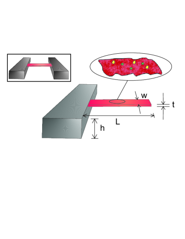
Figure 1: (Color online) Sketch of the systems considered in the text. The inset shows a doubly clamped beam, while the main figure shows a cantilever characterized by its dimensions, width ($w$), thickness ($t$), and length, ($L$), where $w\sim t\ll L$. The height above the substrate is $h$. A schematic view of the surface is given, highlighting imperfections like roughness and adsorbates, which dominate dissipation at low temperatures.

A key figure of merit of the mechanical oscillation is its quality factor $Q=\omega/\Delta\omega$, where $\Delta\omega$ is the measured linewidth of the corresponding vibrational eigenmode of frequency $\omega$. To reach the quantum regime, as well as for most practical applications, where the measured shifts of the resonant frequency $\omega$ constitute the detectors principle, a very high $Q$ is compulsory. Imperfections and the environment surrounding the oscillator result in both a finite linewidth $\Delta\omega$ and a frequency shift $\delta\omega$ with respect to the ideal case. Therefore several works have been devoted to the analysis of the different sources of dissipation present in MEMS and NEMS   Cleland and Roukes (1999); Yasumura et al. (2000); Evoy et al. (2000); Cleland and Roukes (2002); Yang et al. (2002); Mohanty et al. (2002); Ahn and Mohanty (2003); Husain et al. (2003); Zolfagharkhani et al. (2005b); Feng et al. (2006); Shim et al. (2007), trying to determine the dominant damping mechanisms and ways to minimize them. Among the different mechanisms affecting semiconductor-based NEMS the most important and difficult to avoid are i) clamping losses   Jimbo and Itao (1968); Photiadis and Judge (2004), through the transfer of energy from the resonator mode to acoustic modes at the contacts and beyond to the substrate, ii) thermoelastic damping   Zener (1938); Lifshitz and Roukes (2000); De and Aluru (2006) and iii) friction processes taking place at the surfaces   Yang et al. (2000); Liu et al. (2005); Chu et al. (2007). At low temperatures and for decreasing sizes the prevailing mechanism is the last one   Ekinci and Roukes (2005), as indicated by the linear decrease of the quality factor of flexural modes with decreasing size (see fig.[2]), or the sharp increase of $Q$ when the resonator is annealed   Yang et al. (2000); Wang et al. (2004). Excitation of adsorbed molecules, movement of lattice defects or configurational rearrangements absorb irreversibly energy from the excited eigenmode and redistribute it among the rest of degrees of freedom of the system.

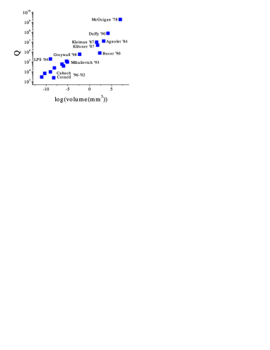
Figure 2: (Color online) From ref.   Ekinci and Roukes (2005). Evolution of reported quality factors in monocrystalline mechanical resonators with size, showing a decrease with linear dimension, i.e., with increasing surface-to-volume ratio, indicating a dominant role of surface-related losses.

A theoretical quantitatively accurate description of surface dissipation proves therefore challenging, as many different dynamical processes and actors come into play, some of whom are not yet well characterized, so simplifications need to be made to provide a unified framework for all of them. In   Seoanez et al. (2007) such a scheme was given, based on the following considerations: i) experimental observations indicate that surfaces of otherwise monocrystalline resonators acquire a certain degree of roughness, impurities and disorder, resembling an amorphous structure   Liu et al. (1999). ii)In amorphous solids the damping of acoustic waves at low temperatures is successfully explained by the Standard Tunneling Model   Anderson et al. (1972); Phillips (1972, 1987); Esquinazi (1998), which couples the acoustic phonons to a set of Two-Level Systems (TLSs) representing the low-energy spectrum of all the degrees of freedom (DoF) able to exchange energy with the strain field associated to the vibration. These DoF correspond to impurities or clusters of atoms within the structure which have in their configurational space two energy minima separated by an energy barrier (similarly to the dextro/levo configurations of the ammonia molecule), modeled as a DoF tunneling between two potential wells. At low temperatures only the two lowest eigenstates have to be considered, characterized by the bias $\Delta^{z}_{0}$ between the wells and the tunneling rate $\Delta^{x}_{0}$ through the barrier. The Standard Tunneling Model specifies the properties of the set of TLSs in terms of a probability distribution $P(\Delta^{x}_{0},\Delta^{z}_{0})$ which can be inferred from general considerations   Anderson et al. (1972); Phillips (1972) and is supported by experiments   Esquinazi (1998). It has to be noted, however, that below a certain temperature the model breaks down due to the increasing role played by interactions among the TLSs, not included   Yu and Leggett (1988); Esquinazi et al. (2004).

In   Seoanez et al. (2007) a description of the attenuation of vibrations in nanoresonators due to their amorphous-like surfaces in terms of an adequate adaptation of the Standard Tunneling Model was intended to be given. An estimate for $Q^{-1}(T)$ was provided, reproducing correctly the weak $\sim T^{1/3}$ temperature dependence as well as the order of magnitude observed in recent experiments   Zolfagharkhani et al. (2005b); Shim et al. (2007). However, the way the Standard Tunneling Model was adapted was not fully correct, and a revision of the results for $Q^{-1}(T)$ obtained therein was mandatory.

In this work we will i) Discuss in detail some important issues hardly mentioned in   Seoanez et al. (2007), ii) Modify some points to obtain a theory fully consistent with the Standard Tunneling Model and which includes all possible dissipative processes due to the presence of TLSs, iii) Extend the results and give expressions for the quality factor of cantilevers as well as damping of torsional modes, and frequency shifts associated, iv) Compare with available experimental data, discussing the validity of the model, range of applicability, aspects to be modified/included to reach an accurate quantitative fit to experiments, v) Study the dissipative effects associated to the presence of metallic electrodes frequently deposited on top of the resonators.

Section II starts with a brief summary of the model described in   Seoanez et al. (2007), discussing the approximations involved, while the different dissipative mechanisms due to the presence of TLSs are presented in III. Section IV analyzes and compares the two main mechanisms, namely relaxational processes associated to asymmetric (biased) TLSs, and non-resonant damping of symmetric TLSs. The extension of the results to cantilevers and torsional modes is given in Section V. A brief account of frequency shifts’ expressions is found in Section VI. In Section VII comparison with experiments and discussion of the applicability, validity and further extensions of the model is made. Section VIII discusses dissipation effects due to the existence of metallic leads coupled to the resonator, which can be coupled to the electrostatic potential induced by trapped charges in the device. Under some circumstances, these effects cannot be neglected. Finally, the main conclusions of our work are given in Section IX. Details of some calculations are provided in the Appendices.

We will not analyze here dissipation due to clamping and thermoelastic losses, which may dominate dissipation in the case of very short beams and strong driving, respectively. We will also not consider direct momentum exchange processes between the carriers in the metallic circuit and the vibrating system  Shytov et al. (2002).

II Surface friction modeled by TLS$\rm{s}$

II.1 Hamiltonian

We will consider a rod of length $L$, width $w$ and thickness $t$, see fig.[1], and use units such that $\hbar=1=k_{B}$. As described in   Seoanez et al. (2007), the vibrating resonator with imperfect surfaces is represented by its vibrational eigenmodes coupled to a collection of non-interacting TLSs, assuming that the main effect of the strain caused by the phonons is to modify the bias $\Delta^{z}_{0}$ of the TLSs   Anderson (1986):

$$H = \sum_{k,j}\omega_{k,j}a_{k,j}^{\dagger}a_{k,j}+$$

$$+ \sum_{\Delta^{x}_{0},\Delta^{z}_{0}}\Bigl{\{}\Delta^{x}_{0}\sigma_{x}+\Bigl{[}\Delta^{z}_{0}+\sum_{k,j}\lambda_{k,j}\left(b_{k,j}^{\dagger}+b_{k,j}\right)\Bigr{]}\sigma_{z}\Bigr{\}}$$

The index $j$ represents the three kinds of modes present in a thin beam geometry   Landau and Lifshitz (1959): flexural (bending), torsional and compression modes. These modes will be present for wavelengths $\lambda>t$, while for shorter ones the system is effectively 3D, with the corresponding 3D modes. The main effect of these high energy 3D modes is to renormalize the tunneling amplitude, so we will take that renormalized value as our starting point $\Delta^{x}_{0}$ and forget in the following about the 3D modes. The sum over TLSs is characterized by the probability distribution $P(\Delta^{x}_{0},\Delta^{z}_{0})=P_{0}/\Delta^{x}_{0}$ .   Anderson et al. (1972); Phillips (1972) This result follows, as explained in   Phillips (1987, 1972), just due to i) the exponential sensitivity of $\Delta^{x}_{0}$ to the properties of the energy barrier of the two-well potential giving rise at low T to the TLS description of the system (resulting in a $1/\Delta^{x}_{0}$ dependence of $P(\Delta^{x}_{0},\Delta^{z}_{0})$), and ii) the characteristic energy scale of the distribution of asymmetries $\Delta^{z}_{0}$, much bigger than 1K, which is the temperature at which experiments are performed, and which thus fixes the scale of the bias of a TLS if it is to contribute significantly to dissipation, $\Delta^{z}_{0}\leq 1$K (therefore the relevant TLSs have values of $\Delta^{z}_{0}$ lying in a very narrow energy range around $\Delta^{z}_{0}=0$ as compared to the variance of their probability distribution, allowing us to consider that $P(\Delta^{x}_{0},\Delta^{z}_{0})$ to a first approximation does not depend on $\Delta^{z}_{0}$). Unphysical divergencies do not appear, as $\Delta^{x}_{0}>\Delta_{min}$, with $\Delta_{min}$ fixed by the typical timescale of the experiment, given by the time needed to obtain a spectrum around the resonance frequency of the excited vibrational eigenmode of the resonator, and $\varepsilon=\sqrt{(\Delta^{x}_{0})^{2}+(\Delta^{z}_{0})^{2}}<\varepsilon_{max}$, estimated to be of the order of 5 K   Esquinazi (1998). For typical amorphous insulators $P_{0}\sim 10^{44}$J^-1m^-3.

To see to which low energy modes the TLSs are more coupled, inducing a more effective dissipation at low temperatures, the spectral function $J(\omega,j)\equiv\sum_{k}\left|\lambda_{k,j}\right|^{2}\delta(\omega-\omega_{k,j})$ characterizing the evolution of the strength of the coupling for each type of mode can be computed. Due to their nonlinear dispersion relation, $\omega=\sqrt{EI/(\rho tw)}k^{2}$, with $I=t^{3}w/12$, $E$ the Young modulus and $\rho$ the mass density, flexural modes show a subohmic behavior $J_{{\rm flex}}(\omega)=\alpha_{b}\sqrt{\omega_{co}}\sqrt{\omega}$, with

$$\alpha_{b}\sqrt{\omega_{co}}=0.3\frac{\gamma^{2}}{t^{3/2}w}\frac{(1+\nu)(1-2\nu)}{E(3-5\nu)}\Bigl{(}\frac{\rho}{E}\Bigr{)}^{1/4}\,,$$ (2)

where $\gamma\sim 5$ eV is a coupling constant appearing in $\lambda_{k,j}$, $\nu$ is Poisson’s ratio and $\omega_{co}\simeq\sqrt{EI/(\rho tw)}(2\pi/t)^{2}$ is the high energy cut-off of the bending modes. A detailed derivation of $J_{{\rm flex}}(\omega)$ is given in Appendix A. Even though the length $L$ of our system is finite, and thus the vibrational spectrum discrete, a continuum approximation like this one will hold if $kT\gg\hbar\omega_{fund}$, $\omega_{fund}$ being the frequency of the fundamental mode.

The bending modes prevail over the other, ohmic-like, modes as a dissipative channel at low energies, thanks to their weaker $J_{{\rm flex}}(\omega)\sim\omega^{1/2}$ dependence. One may ask at what frequency do the torsional and compression modes begin to play a significant role, and a rough way to estimate it is to see at what frequency do the corresponding spectral functions have the same value, $J_{{\rm flex}}(\omega*)=J_{{\rm comp,tors}}(\omega*)$. Using the expressions in Seoanez et al. (2007), namely $J_{{\rm comp,tors}}(\omega)=\alpha_{c,t}\omega$, with $\alpha_{c}=(\gamma\Delta_{0}^{x}/\Delta_{0})^{2}(2\pi^{2}\rho tw)^{-1}(E/\rho)^{-3/2}$ and $\alpha_{t}=C(\gamma\Delta_{0}^{x}/\Delta_{0})^{2}(8\pi^{2}\mu tw\rho I)^{-1}(\rho I/C)^{3/2}$, the results are $\omega*\sim 30(1+\nu)^{2}(1-2\nu)^{2}(E/\rho)^{1/2}/[t(3-5\nu)^{2}]$ for the case of compression modes and $\omega*\sim 300(1-2\nu)^{2}(E/\rho)^{1/2}/[t(3-5\nu)^{2}(1+\nu)]$ for the torsional. Comparing these frequencies to the one of the onset of 3D behavior, $\omega_{co}$, they are similar, justifying a simplified model where only flexural modes are considered.

II.2 TLSs dynamics

The interaction between the bending modes and the TLSs affects both of them. When a single mode is externally excited, as is done in experiments, the coupling to the TLSs will cause an irreversible energy flow, from this mode to the rest of the modes through the TLSs, as depicted in fig.(3a). The dynamics of the TLSs in presence of the vibrational bath determines the efficiency of the energy flow and thus the quality factor of the excited mode. Taking a given TLS plus the phonons, its dynamics is characterized by the Fourier transform of the correlator $\langle\sigma_{z}(t)\sigma_{z}(0)\rangle$, the spectral function $A(\omega)$, which at $T=0$ reads

$$A(\omega)\equiv\sum_{n}\left|\left\langle 0\left|\sigma_{z}\right|n\right\rangle\right|^{2}\delta(\omega-\omega_{n}+\omega_{0})$$ (3)

where $|n\rangle$ is an excited state of the total system TLS plus vibrations. In   Seoanez et al. (2007) an analysis of $A(\omega)$ was made for the case of a symmetric TLS ($\Delta^{z}_{0}=0$), concluding that i)If $\Delta^{x}_{0}\ll\alpha_{b}^{2}\omega_{co}$ the tunneling amplitude is basically suppressed and the TLS does not participate in dissipative processes. For reasonable system dimensions the coupling constant is very small, $\alpha_{b}\ll 1$, so this effect can be ignored, ii)Around the resonance at $\omega=\Delta^{x}_{0}$ a broadening appears, $\Gamma(\Delta^{x}_{0})$ which, for $\Gamma(\Delta^{x}_{0})\ll\Delta^{x}_{0}$ is given by the Fermi Golden Rule result $\Gamma(\Delta^{x}_{0})=16\alpha_{b}\sqrt{\omega_{co}}\,\sqrt{\Delta^{x}_{0}}$ (for $T=0$ K, at $T>0$ eq.(7) applies), iii)The coupling to phonons of all energies provides the ”dressed” TLS with tails far from resonance, $A(\omega)\propto\alpha_{b}\sqrt{\omega_{co}\omega}/(\Delta^{x}_{0})^{2}$ for $\omega\ll\Delta^{x}_{0}$ and $A(\omega)\propto\alpha_{b}\sqrt{\omega_{co}}(\Delta^{x}_{0})^{2}\omega^{-7/2}$, for $\omega\gg\Delta^{x}_{0}$, see left side of fig.(3b), iv) The main effect of the asymmetry $\Delta^{z}_{0}$ is to suppress the TLSs dynamics, so the TLSs playing an active role in dissipation satisfy $\Delta^{x}_{0}>|\Delta^{z}_{0}|$.

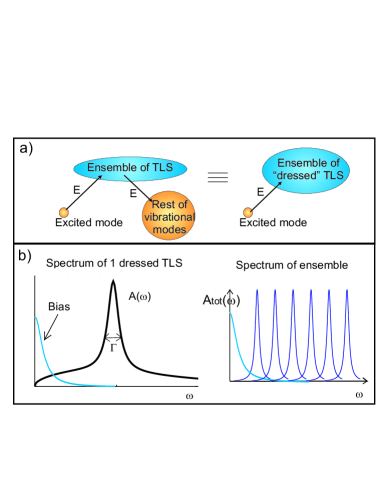
Figure 3: (Color online)a) Schematic representation of the irreversible flow of energy from the externally excited mode to the TLS ensemble, and from the ensemble to the rest of vibrational modes. This process can be viewed as a flow of energy from the excited mode to an ensemble of ”dressed” TLSs, with their dynamics modified by the presence of the vibrational modes. b) Left: Spectral function $A(\omega)$ of a single dressed TLS, weakly damped ($\Gamma<\Delta^{x}_{0}$). A peak around $\omega=0$ arises if the system is biased, corresponding to the relaxational dissipation mechanism. Right: Total spectral function $A_{tot}(\omega)$ of the ensemble of dressed TLSs.

Finally, for those low-energy overdamped TLSs such that $\Gamma(\Delta^{x}_{0})\gg\Delta^{x}_{0}$ an incoherent decay $\exp(-t/\tau)$ with time, with $\tau(\Delta^{x}_{0})=\Gamma(\Delta^{x}_{0})^{-1}$ was assumed.

Two points that ref.  Seoanez et al. (2007) missed, and now will be considered, are the following: First, the effect of the asymmetry is not simply the one stated. An underdamped biased TLS develops an additional peak around $\omega=0$, as shown in fig.(3b), which corresponds to the relaxation mechanism that dominates dissipation of acoustic waves in amorphous solids   Esquinazi (1998), see eq.(9). In   Seoanez et al. (2007) the relaxation mechanism associated to eq.(9) was misinterpreted to correspond to friction due to overdamped TLSs, while in this work it will be, consistently with the Standard Tunneling Model, linked to the presence of biased underdamped TLSs. It will be described in more detail in the next section, and taken into account in the computation of the total dissipation.

Second point missed by ref.  Seoanez et al. (2007): one can estimate, using the probability distribution $P(\Delta^{x}_{0},\Delta^{z}_{0})$, the total number of overdamped TLSs in the volume fraction of the resonator presenting amorphous features, $V_{amorph}$. With $V_{amorph}\sim V_{tot}/10$, and using $\Gamma(E,T)=\Gamma(E,T=0)\coth[E/2T]\approx 2T\Gamma(E,T=0)/E$, the number of overdamped TLSs, $\Delta^{x}_{0}\leq\Gamma(\Delta^{x}_{0},T)\rightarrow\Delta^{x}_{0}\leq[30\alpha_{b}\sqrt{\omega_{co}}T]^{2/3}$, is $N\approx P_{0}twL[30\alpha_{b}\sqrt{\omega_{co}}T]^{2/3}$, which for typical resonator sizes $L\sim 1\mu$m, $t,w\sim 0.1\mu$m is less than one for $T<1$K. Therefore, unless the resonator is bigger and/or $P_{0}$ too, this contribution to dissipation can be safely neglected, as it will be done in the following.

III Dissipative mechanisms

From the features of the spectral function $A_{tot}(\omega)=\sum_{\Delta^{x}_{0},\Delta^{z}_{0}}A(\Delta^{x}_{0},\Delta^{z}_{0},\omega)$ of the ensemble of dressed TLSs, one can classify into three kinds the dissipative mechanisms affecting an externally excited mode $\omega_{0}$:

III.1 Resonant dissipation

Those TLSs with their unperturbed excitation energies close to $\omega_{0}$ will resonate with the mode, exchanging energy quanta, with a rate proportional to the mode’s phonon population $n_{\omega_{0}}$ to first order. For usual excitation amplitudes $\sim 1$Å the vibrational mode is so populated (as compared with the thermal population) that the resonant TLSs become saturated, and their contribution to the transverse (flexural) wave attenuation becomes negligible, proportional to $n_{\omega_{0}}^{-1/2}\,\,\,\,$   Arnold et al. (1974).

III.2 Dissipation of symmetric non-resonant TLSs

We show first that a correct description of the dissipation due to weakly damped TLSs is given by the approximate Hamiltonian used in   Seoanez et al. (2007), starting from eq.(II.1), if one considers apart in some way the presence of the relaxational peak at $\omega=0$ due to a finite bias $\Delta^{z}_{0}\neq 0$.

We focus the attention on a given TLS plus the vibrations (spin-boson model), $\textsl{H}=\Delta^{x}_{0}\sigma_{x}+\Delta^{z}_{0}\sigma_{z}+H_{int}+H_{vibr}$,

$$H_{int}=\sigma_{z}\sum_{k}\lambda\frac{k^{2}}{\sqrt{\omega_{k}}}(a^{\dagger}_{k}+a_{k})$$ (4)

with $\lambda$ defined in eq.(36). In   Seoanez et al. (2007) a change of basis to the unperturbed eigenstates of the TLS was performed, obtaining $\textsl{H}=\varepsilon\sigma_{z}+[(\Delta^{x}_{0}/\varepsilon)\sigma_{x}+(\Delta^{z}_{0}/\varepsilon)\sigma_{z}]\sum_{k}\lambda\frac{k^{2}}{\sqrt{\omega_{k}}}(a^{\dagger}_{k}+a_{k})+H_{vibr}$. Then the term $(\Delta^{z}_{0}/\varepsilon)\sigma_{z}$ was ignored (remember $\varepsilon=\sqrt{(\Delta^{x}_{0})^{2}+(\Delta^{z}_{0})^{2}}$), arguing that the key role in dissipation is played by fairly symmetrical TLSs, $|\Delta^{z}_{0}|\ll\varepsilon$. This allowed to simplify the spin-boson Hamiltonian to the one of a symmetric TLS, much easier to analyze, with tunneling amplitude $\varepsilon$ instead of $\Delta^{x}_{0}$ and coupling $\lambda(\Delta^{x}_{0}/\varepsilon)$ instead of $\lambda$. The consistency was kept by restricting the sums over the TLS ensemble to those such that $|\Delta^{z}_{0}|\leq\Delta^{x}_{0}$.

One can check this consistency going back to the original basis, where the approximation of the Hamiltonian reads $\textsl{H}\approx\Delta^{x}_{0}\sigma_{x}+\Delta^{z}_{0}\sigma_{z}+[(\Delta^{x}_{0}/\varepsilon)^{2}\sigma_{z}-(\Delta^{z}_{0}\Delta^{x}_{0}/\varepsilon^{2})\sigma_{x}]\sum_{k}\lambda\frac{k^{2}}{\sqrt{\omega_{k}}}(a^{\dagger}_{k}+a_{k})+H_{vibr}$. Restricting the application of this Hamiltonian to those TLSs such that $|\Delta^{z}_{0}|\leq\Delta^{x}_{0}$ seems to be a fairly good approximation, but a price has been paid, namely the spectral weight at $\omega=0$ due to the bias has been lost in this effectively symmetric spin-boson approximation. This weight cannot be ignored, and it has to be added as a different mechanism (the relaxational mechanism), what will be done in the next subsection. Once this issue has been taken care off, all the dissipative processes due to the presence of TLSs are correctly included in this framework, and we can proceed describing non-relaxational friction due to non-resonant, weakly damped, weakly biased TLSs.

As mentioned before, the coupled system TLSs + vibrations can be viewed, taking the coupling as a perturbation, from the point of view of the excited mode $\omega_{0}$ as a set of TLSs with a modified absorption spectrum. The TLSs, dressed perturbatively by the modes, are entities capable of absorbing and emitting over a broad range of frequencies, transferring energy from the excited mode $\omega_{0}$ to other modes. The contribution to the value of the inverse of the quality factor, $Q^{-1}(\omega_{0})$, of all these non-resonant TLSs will be proportional to $A_{\rm{off-res}}^{\rm{tot}}(\omega_{0})=\sum_{\Delta^{x}_{0}=0}^{\omega_{0}-\Gamma(\omega_{0})}A(\Delta^{x}_{0},\Delta^{z}_{0},\omega_{0})+\sum_{\omega_{0}+\Gamma(\omega_{0})}^{\varepsilon_{max}}A(\Delta^{x}_{0},\Delta^{z}_{0},\omega_{0})\approx 2P\alpha_{b}\sqrt{\omega_{co}/\omega_{0}}$ , a quantity measuring the density of states which can be excited through $H_{\rm{int}}$ at frequency $\omega_{0}$, see Appendix B for details.

For an excited mode $\omega_{0}$ populated with $n_{\omega_{0}}$ phonons, $Q^{-1}(\omega_{0})$ is given by $Q^{-1}(\omega_{0})=\Delta E/2\pi E_{0}$, where $E_{0}$ is the energy stored in the mode per unit volume, $E_{0}\simeq n_{\omega_{0}}\hbar\omega_{0}/twL$, and $\Delta E$ is the energy fluctuations per cycle and unit volume. $\Delta E$ can be obtained from Fermi Golden Rule:

$$\Delta E_{\rm{off-res}}^{\rm{tot}}\simeq\frac{2\pi}{\omega_{0}}\times\hbar\omega_{0}\times\frac{2\pi}{\hbar}n_{\omega_{0}}\left(\lambda\frac{k_{0}^{2}}{\sqrt{\omega_{0}}}\right)^{2}A_{\rm{off-res}}^{\rm{tot}}(\omega_{0})\,,$$ (5)

and the inverse quality factor of the vibration follows. For finite temperatures the calculation of $A_{\rm{off-res}}^{\rm{tot}}(\omega_{0},T)$ is done in Appendix B. The result, valid for temperatures below the breakdown of the TLS approximate description of the two-well potential ($T\sim 5$K  Esquinazi (1998)), is different from the one given in   Seoanez et al. (2007), because there the value of $Q^{-1}(\omega_{0},T)$ was interpreted as corresponding to the net energy loss of the studied mode (subtracting emission processes from absorption ones), while in experiments the observed linewidth is due to the total amount of fluctuations, the addition of emission and absorption processes. So in this context dissipation means fluctuations, and not net loss of energy. The contribution of these kind of processes is thus

$$(Q^{-1})_{\rm{off-res}}^{\rm{tot}}(\omega_{0},T)\simeq 10P_{0}t^{3/2}w\left(\frac{E}{\rho}\right)^{1/4}\frac{\alpha_{b}^{2}\omega_{co}}{\omega_{0}}\rm{cotanh}\Bigl{[}\frac{\omega_{0}}{T}\Bigr{]}$$ (6)

III.3 Contribution of biased TLSs to the linewidth: relaxation absorption

This very general friction mechanism arises due to the phase delay between stress and imposed strain rate. In our context, for a given TLS the populations of its levels take a finite time to readjust when a perturbation changes the energy difference between its eigenstates   Jäckle (1972); Esquinazi (1998). This time $\tau$ corresponds to the inverse linewidth and is given, for not too strong perturbations, by the Fermi Golden Rule result

$$\Gamma(\varepsilon,T)=16\alpha_{b}\sqrt{\omega_{co}}\times\sqrt{\varepsilon}\coth[\varepsilon/2T]$$ (7)

where $\varepsilon=\sqrt{(\Delta^{x}_{0})^{2}+(\Delta^{z})^{2}}$ is the energy difference between the levels. Notice that $\Delta^{z}$ is not just the bare $\Delta^{z}_{0}$ appearing in the Hamiltonian of the system, but the net bias including the modification due to the coupling to the vibrational modes, $\Delta^{z}=\Delta^{z}_{0}+\xi_{k}\partial u_{k}$ ($\xi_{k}$ is the corresponding coupling constant with the proper dimensions and $\partial u_{k}$ a component $k$ of the deformation gradient matrix, defined recalling eq.(4) as $\partial u_{k}\sim\langle k,n_{k}|(k/\sqrt{\omega_{k}})(a^{\dagger}_{k}+a_{k})|k,n_{k}\rangle$, associated to a vibrational mode $|k,n_{k}\rangle$). Eq.(7) is valid in the range of applicability of the TLS description of the two well potentials ($T\leq 5$K), and for values of $\alpha_{b}$ such that $\Gamma(\varepsilon,T)<\varepsilon$. Therefore the energy levels $\varepsilon_{1,2}=\mp\frac{1}{2}\sqrt{(\Delta^{x}_{0})^{2}+(\Delta^{z})^{2}}=\mp\frac{1}{2}\sqrt{(\Delta^{x}_{0})^{2}+(\Delta^{z}_{0}+\xi_{k}\partial u_{k})^{2}}$ depend on $\partial u_{k}$, and to first order the sensitivity of these energies to an applied strain is proportional to the bias

$$\frac{\partial\varepsilon_{i}}{\partial(\partial u_{k})}=\frac{(\Delta^{z}_{0}\mp\xi_{k}\partial u_{k})}{\varepsilon_{i}}\xi_{k}=\frac{\Delta_{z}^{tot}}{\varepsilon_{i}}\xi_{k}\,\,\,,$$ (8)

with a response of the TLS $\propto(\Delta^{z}/\varepsilon)^{2}$. In   Esquinazi (1998) a detailed derivation is given, and the imaginary part of the response, corresponding to $Q^{-1}$ is also $\propto\tau/(1+\omega^{2}\tau^{2})$, which in terms of $A(\omega)$ is the lorentzian peak at $\omega=0$ of fig(3b).

The mechanism is most effective when $\tau\sim 1/\omega$, where $\omega$ is the frequency of the vibrational mode; then, along a cycle of vibration, the following happens (see fig.(4)): When the TLS is under no stress the populations, due to the delay $\tau$ in their response, are being still adjusted as if the levels corresponded to a situation with maximum strain (and therefore of maximum energy separation between them, cf. $\varepsilon_{1,2}(u_{k})$), so that the lower level becomes overpopulated. As the strain is increased to its maximum value the populations are still adjusting as if the levels corresponded to a situation with minimum strain, thus overpopulating the upper energy level. Therefore in each cycle there is a net absorption of energy from the mechanical energy pumped into the vibrational mode.

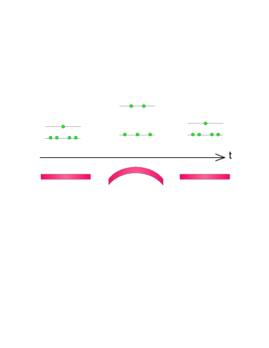
Figure 4: (Color online) Schematic representation of the levels’ population evolution of an ensemble of 5 identical TLSs with a response time $\tau\sim 1/\omega$, where $\omega$ is the frequency of the bending mode excited, whose evolution is also depicted in the lower part of the figure. The delay $\tau$ plus the bias $\Delta^{z}_{0}$ give rise to the relaxational energy loss mechanism of the mode, see text.

If on the other hand $\tau\gg 1/\omega$ the TLSs levels’ populations are frozen with respect to that fast perturbation, while in the opposite limit $\tau\ll 1/\omega$ the levels’ populations are always in instantaneous equilibrium with the variations of $\varepsilon_{1,2}$ and there is neither a net absorption of energy.

For an ensemble of TLSs, the contribution to $Q^{-1}$ is   Esquinazi (1998)

$$Q^{-1}_{\rm{rel}}(\omega,T) = P_{0}\gamma^{2}/(ET)\smallint_{0}^{\varepsilon_{max}}d\varepsilon\smallint_{u_{min}}^{1}du\sqrt{1-u^{2}}/u\times$$ (9)

$$\times \frac{1}{\cosh^{2}\left(\varepsilon/2T\right)}\frac{\omega\tau}{1+(\omega\tau)^{2}}$$

The derivation of eq.(9) only relies in the assumptions of an existence of well defined levels who need a finite time $\tau$ to reach thermal equilibrium when a perturbation is applied, and the existence of bias $|\Delta^{z}_{0}|>0$. This implies that such a scheme is applicable also to our 1D vibrations, but is valid only if the perturbation induced by the bath on the TLSs is weak, so that the energy levels are still well defined. Therefore we will limit the ensemble to underdamped TLSs for whom $\Gamma(\varepsilon,T)<\varepsilon$. In eq.(9) the factor $\cosh^{-2}\left(\varepsilon/2T\right)$ imposes an effective cutoff $\varepsilon<T$, so that in eq.(7) one can approximate $\coth[\varepsilon/2T]\sim 2T/\varepsilon$, resulting in $\Gamma(\varepsilon)\sim 1/\sqrt{\varepsilon}$, and thus the underdamped TLSs will satisfy $\varepsilon\geq[30\alpha_{b}\sqrt{\omega_{co}}T]^{2/3}$. For $T\gg[32\alpha_{b}\sqrt{\omega_{co}}]^{2}$, which is fulfilled for typical sizes and temperatures (see Appendix C for details)

$$Q^{-1}_{\rm{rel}}(\omega_{0},T)\approx\frac{20P_{0}\gamma^{4}}{t^{3/2}w}\frac{(1+\nu)(1-2\nu)}{E^{2}(3-5\nu)}\Bigl{(}\frac{\rho}{E}\Bigr{)}^{1/4}\frac{\sqrt{T}}{\omega_{0}}$$ (10)

Here $V_{amorph}\sim V_{tot}/10$ was assumed.

IV Comparison between contributions to $Q^{-1}$. Relaxation prevalence.

It is useful to estimate the relative importance of the contributions to $Q^{-1}$ coming from the last two mechanisms. For that sake, we particularize the comparison to the case of the fundamental flexural mode, which is the one usually excited and studied, of a doubly clamped beam, with frequency $\omega_{0}\approx 6.5(E/\rho)^{1/2}t/L^{2}$ (for a cantilever these considerations hold, with only a slight modification of the numerical prefactors; the conclusions are the same). The result is:

$$\Bigl{[}\frac{Q^{-1}_{\rm{rel}}(T)}{Q^{-1}_{\rm{off-res}}(T)}\Bigr{]}_{\rm{fund}}\approx\frac{300t^{1/2}}{L}\frac{(3-5\nu)}{(1+\nu)(1-2\nu)}\frac{E}{\rho}\frac{1}{T^{1/2}}$$ (11)

For a temperature $T=1$K, the result is as big as $10^{6}$ even for a favorable case $t=1$nm, $L=1\mu$m, $E=50$GPa, $\nu=0.2$, $\rho=3$g/cm³. So for any reasonable temperature and dimensions the dissipation is dominated by the relaxation mechanism, so that the prediction of the limit that surfaces set on the quality factor of nanoresonators is, within this model for the surface, eq.(10):

$$Q^{-1}_{\rm{surface}}(\omega_{0},T)\approx Q^{-1}_{\rm{rel}}(\omega_{0},T)\sim\frac{T^{1/2}}{\omega_{0}}$$ (12)

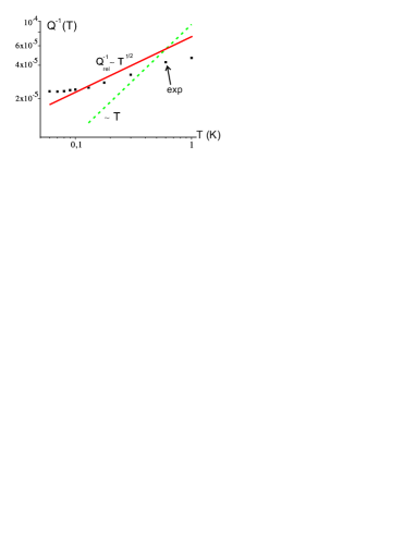
Figure 5: (Color online) Example of fit of $Q^{-1}_{\rm{rel}}(\omega_{0},T)$, eq.(10), to experimental data. The data correspond to a Si resonator vibrating at $\omega_{0}=12.028$ MHz, see ref. Zolfagharkhani et al. (2005b). Although the predicted order of magnitude for the dissipation and the sublinear temperature dependence is observed, the experimental trend follows a weaker temperature dependence than the prediction $T^{1/2}$. For comparison a linear temperature dependence is shown (dotted line). See the text for more details.

For typical values $L\sim 1\mu$m, $t,w\sim 0.1\mu$m, $\gamma\sim 5$ eV, $P_{0}V_{amorph}/V_{tot}\sim 10^{44}$J/m³, and T in the range 1mK-0.5K the estimate for $Q^{-1}_{\rm{surface}}\sim 10^{-4}$ gives the observed order of magnitude in experiments like   Zolfagharkhani et al. (2005b), and also predicts correctly a sublinear dependence, but with a higher exponent, $1/2$ versus the experimental fit $0.36$ in   Zolfagharkhani et al. (2005b) or $0.32$ in   Shim et al. (2007), see fig.(5) for an example.

V Extensions to other devices

V.1 Cantilevers, nanopillars and torsional oscillators

The extrapolation from doubly clamped beams to cantilevers   Mukhopadhyay et al. (2005) and nanopillars   Scheible and Blick (2004) is immediate, the only difference between them being the allowed (k,$\omega$(k)) values due to the different boundary conditions at the free end (and even this difference disappears as one considers high frequency modes, where in both cases one has $k_{n}\approx(2n+1)\pi/2L$). All previous results apply, and one has just to take care in the expressions corresponding to the $Q^{-1}$ of the fundamental mode, where there is more difference between the frequencies of both cases, the cantilever one being $\omega_{0}^{cant}\approx(E/\rho)^{1/2}t/L^{2}$ as compared to the doubly clamped case, $\omega_{0}^{clamped}\approx 6.5(E/\rho)^{1/2}t/L^{2}$.

V.2 Effect of the flexural modes on the dissipation of torsional modes

The contribution from the TLSs + subohmic bending mode environment to the dissipation of a torsional mode of a given oscillator can be also estimated. We will study the easiest (and experimentally relevant  Sharos et al. (2004)) case of a cantilever. For paddle and double paddle oscillators the geometry is more involved, modifying the moment of inertia and other quantities. When these changes are included, the analysis follows the same steps we will show.

Relaxation absorption. We assume, based on the previous considerations on the predominant influence of the flexural modes on the TLSs dynamics, as compared with the influence of the other modes, that the lifetime $\tau=\Gamma^{-1}$ of the TLSs is given by eq.(7). The change in the derivation of the expression for $Q^{-1}$ comes in eq.(8), where the coupling constant $\xi_{k}^{\rm{tors}}$ is different, which translates simply, in eq.(9), into substituting $\gamma^{2}\leftrightarrow\gamma_{\rm{tors}}^{2}$, and the corresponding prediction for $Q^{-1}_{\rm{rel}}$

$$Q^{-1}_{\rm{rel}}(\omega_{0},T)\approx\frac{20P_{0}\gamma_{\rm{tors}}^{2}\gamma^{2}}{t^{3/2}w}\frac{(1+\nu)(1-2\nu)}{E^{2}(3-5\nu)}\Bigl{(}\frac{\rho}{E}\Bigr{)}^{1/4}\frac{\sqrt{T}}{\omega_{0}}\,,$$ (13)

where now $\omega_{0}$ is the frequency of the corresponding flexural mode. The range of temperatures and sizes for which this result applies is the same as in the case of an excited bending mode.

Dissipation of symmetric non-resonant TLSs The modified excitation spectrum of the TLS’s ensemble, $A_{\rm{off-res}}^{\rm{tot}}(\omega_{0},T)$, remains the same, and the change happens in the matrix element of the transition probability of a mode $|k_{0},n_{0}\rangle$ appearing in eq.(5), $(\lambda k_{0}^{2}/\sqrt{\omega_{0}})^{2}$. The operator yielding the coupling of the bath to the torsional mode which causes its attenuation is the interaction term of the Hamiltonian, which for twisting modes is (see Appendix D for the derivation of eqs.(14)-(15))

$$H_{int}^{tors}=\hbar\sigma_{z}\sum_{k}\gamma\sqrt{\frac{C}{8\mu tw}}\sqrt{\frac{1}{2\rho I\hbar L}}\frac{k}{\sqrt{\omega_{k}}}(a^{\dagger}_{k}+a_{k})\,,$$ (14)

where $\mu=E/[2(1+\nu)]$ is a Lande coefficient, and $C=\mu t^{3}w/3$ is the torsional rigidity. Again, $Q^{-1}(\omega_{j})=\Delta E/2\pi E_{0}$, where the energy $E_{0}$ stored in a torsional mode $\phi_{j}(z,t)=A\sin[(2j-1)\pi z/(2L)]\sin(\omega_{j}t)$ per unit volume is $E_{0}=A^{2}\omega_{j}^{2}\rho(t^{2}+w^{2})/48$ ($z$ is the coordinate along the main axis of the rod). Expressing the amplitude $A$ in terms of phonon number $n_{j}$, the energy stored in mode $|k_{j},n_{j}\rangle$ is

$$E_{0}(k_{j},n)=\frac{1}{2}\frac{\hbar\omega_{j}}{(t^{3}w+w^{3}t)L}(t^{2}+w^{2})(2n_{j}+1)\,,$$ (15)

the energy fluctuations in a cycle of such a mode is

$$\Delta E=\frac{2\pi}{\omega_{j}}\times\hbar\omega_{j}\times\frac{2\pi}{\hbar}\frac{\gamma^{2}\hbar\omega_{j}}{16Ltw\mu}n_{j}A_{\rm{off-res}}^{\rm{tot}}(\omega_{j},T)\,,$$ (16)

and the inverse quality factor

$$(Q^{-1})_{\rm{off-res}}^{\rm{tot}}(\omega_{0},T) \approx 0.04\frac{\gamma^{4}P}{t^{3/2}w}\frac{\rho^{1/4}(1+\nu)^{2}(1-2\nu)}{E^{9/4}(3-5\nu)}\times$$ (17)

$$\times\frac{1}{\sqrt{\omega_{0}}}\rm{cotanh}\Bigl{[}\frac{\omega_{0}}{T}\Bigr{]}\,,$$

For sizes and temperatures as the ones used for previous estimates the relaxation contribution dominates dissipation.

VI Frequency shift

Once the quality factor is known the relative frequency shift can be obtained via a Kramers-Kronig relation (valid in the linear regime), because both are related to the imaginary and real part, respectively, of the acoustic susceptibility. First we will demonstrate this, and afterwards expressions for beam and cantilever will be derived and compared to experiments.

VI.1 Relation to the acoustic susceptibility

In absence of sources of dissipation, the equation for the bending modes is given by $-(12\rho/t^{2})\partial^{2}X/\partial t^{2}=E\partial^{4}X/\partial z^{4}$. The generalization in presence of friction is

$$-\frac{12\rho}{t^{2}}\frac{\partial^{2}X}{\partial t^{2}}=(E+\chi)\frac{\partial^{4}X}{\partial z^{4}}$$ (18)

Where $\chi$ is a complex-valued susceptibility. Inserting a solution of the form $X(z,t)=Ae^{i(kx-\omega t)}$, where k is now a complex number, one gets the dispersion relation $\omega=\sqrt{t^{2}(E+\chi)/(12\rho)}k^{2}$. Now, assuming that the relative shift and dissipation are small, implying $\rm{Re}(\chi)<<E$ , $\rm{Im}(k)<<\rm{Re}(k)$, the following expressions for the frequency shift and inverse quality factor are obtained in terms of $\chi$:

$$\left\{\begin{array}[]{ll}Q^{-1}&=\Delta\omega/\omega=-\rm{Im}(\chi)/E\\ \delta\omega/\omega&=\rm{Re}(\chi)/2E\end{array}\right.$$ (19)

Therefore a Kramers-Kronig relation for the susceptibility can be used to obtain the relative frequency shift:

$$\frac{\delta\omega}{\omega}(\omega,T)=-\frac{1}{2\pi}P\int_{-\infty}^{\infty}d\omega^{\prime}\frac{Q^{-1}(\omega^{\prime},T)}{\omega^{\prime}-\omega}\,\,,$$ (20)

where $P$ means here the principal value of the integral.

VI.2 Expressions for the frequency shift

Relaxation processes of biased, underdamped TLSs dominate the perturbations of the ideal response of the resonator, as we have already shown for the inverse quality factor. For most of the frequency range, $\omega\geq[30\alpha_{b}\sqrt{\omega_{co}}T]^{2/3}$, $Q^{-1}(\omega,T)\approx A\sqrt{T}/\omega$ , with $A$ defined by eq.(10). The associated predicted contribution to the frequency shift, using eq.(20), is

$$\frac{\delta\omega}{\omega}(\omega,T)\approx-\frac{A}{2\pi}\frac{\sqrt{T}}{\omega}\log\Bigl{[}\Bigl{|}1-\frac{\omega}{[30\alpha_{b}\sqrt{\omega_{co}}T]^{2/3}}\Bigr{|}\Bigr{]}$$ (21)

For low temperatures, $\omega\gg[30\alpha_{b}\sqrt{\omega_{co}}T]^{2/3}$, the negative shift grows towards zero as $\delta\omega/\omega(\omega,T)\sim\sqrt{T}\log[T^{2/3}/\omega]$, reaching at some point a maximum value, and decreasing for high temperatures, $\omega<[30\alpha_{b}\sqrt{\omega_{co}}T]^{2/3}$, as $\delta\omega/\omega(\omega,T)\sim 1/T^{1/6}$. Even though the prediction of a peak in $\delta\omega/\omega(T)$ qualitatively matches the few experimental results currently available   Zolfagharkhani et al. (2005b); Shim et al. (2007), it does not fit with them quantitatively.

VII Applicability and further extensions of the model. Discussion

As mentioned, the predictions obtained within this theoretical framework do match qualitatively experimental results in terms of observed orders of magnitude for $Q^{-1}(T)$, weak sublinear temperature dependence, and presence of a peak in the frequency shift temperature dependence. But quantitative fitting is still to be reached, while on the experimental side more experiments need to be done at low temperatures to confirm the, until now, few results  Zolfagharkhani et al. (2005b).

Applicability. The several simplifications involved in the model put certain constraints, some of which are susceptible of improvement. We enumerate them first and discuss some of them afterwards: i) The probability distribution $P(\Delta^{x}_{0},\Delta^{z}_{0})$, borrowed from amorphous bulk systems, may be different for the case of the resonator’s surface, ii) The assumption of non-interacting TLSs, only coupled among them in an indirect way through their coupling to the vibrations, breaks down at low enough temperatures, where also the discreteness of the vibrational spectrum affects our predictions iii) When temperatures rise above a certain value, high energy phonons with 3D character dominate dissipation, the two-state description of the degrees of freedom coupled to the vibrations is not a good approximation, and thermoelastic losses begin to play an important role, iv) For strong driving, anharmonic coupling among modes has to be considered, and some steps in the derivation of the different mechanisms, which assumed small perturbations, must be modified. This will be the case of resonators driven to the nonlinear regime, where bistability and other phenomena take place.

The solution to issue i) is intimately related to a better knowledge of the surface and the different physical processes taking place there. Recent studies try to shed some light on this question  Chu et al. (2007), and from their results a more realistic $P(\Delta^{x}_{0},\Delta^{z}_{0})$ could be derived, which remains for future work. Before that point, it is easier to wonder about the consequences of a dominant kind of dissipative process which corresponded to a set of TLSs with a well defined value of $\Delta^{x}_{0}$ and a narrow distribution of $\Delta^{z}_{0}$’s of width $\Delta_{1}$, as was suggested for single-crystal silicon  Phillips (1988). Following   Phillips (1988), a $Q^{-1}(T)\sim\sqrt{T}$ behavior is obtained for low temperatures $T<\Delta_{1}$ if $\Gamma(\Delta^{x}_{0},T)<\omega$, and a $Q^{-1}(T)\sim 1/\sqrt{T}$ if $\Gamma(\Delta^{x}_{0},T)>\omega$, while at high temperatures $T>\Delta_{1}$ a constant $Q^{-1}(T)\sim Q_{0}$ is predicted for both cases. These predictions do not match better with experiments than the results obtained with $P(\Delta^{x}_{0},\Delta^{z}_{0})\sim P_{0}/\Delta^{x}_{0}$, so issue i) remains open. From the point of view of those who attribute the origin of the low energy TLSs to the long range interaction between localized defects, a possible source of change for $P(\Delta^{x}_{0},\Delta^{z}_{0})$ may be the decrease in size of the resonator below the correlation length of this interaction.

We try now to have a first estimate of the temperature for which interactions between TLSs cannot be ignored. Following the ideas presented in   Esquinazi (1998), we will estimate the temperature $T*$ at which the dephasing time $\tau_{\rm{int}}$ due to interactions is equal to the lifetime $\tau(T)=\Gamma^{-1}(T)$ defined in eq.(7), for the TLSs that contribute most to dissipation, which are those with $\varepsilon=\sqrt{(\Delta^{x}_{0})^{2}+(\Delta^{z}_{0})^{2}}\sim\Delta^{x}_{0}\sim T$. For them $\tau^{-1}(T)=\Gamma(T)\approx 40\alpha_{b}\sqrt{\omega_{co}}\sqrt{T}$. The interactions between the TLSs are dipolar, described by $H_{\rm{int}}=\sum_{i,j}U_{1,2}\sigma_{1}^{z}\sigma_{2}^{z}$, with $U_{1,2}=b_{12}/r_{12}^{3}$, $b_{12}$ verifying $\langle b_{12}\rangle\approx 0$, $\langle|b_{12}|\rangle\equiv U_{0}\approx\gamma^{2}/E$   Yu and Leggett (1988); Esquinazi (1998). From the point of view of a given TLS the interaction affects its bias, $\Delta_{j}^{z}=(\Delta^{z}_{0})_{j}+\sum_{i}U_{ij}\sigma_{j}^{z}$, causing fluctuations of its phase $\delta\varepsilon_{j}(t)$ (where $t$ here means time and not thickness), which have an associated $\tau_{\rm{int}}$ defined by $\delta\varepsilon_{j}(\tau_{\rm{int}})\tau_{\rm{int}}\sim 1$. These fluctuations are caused by those TLSs which, within the time $\tau_{\rm{int}}$, have undergone a transition between their two eigenstates, affecting through the interaction $H_{\rm{int}}$ the value of the bias of our TLS. At a temperature $T$, the most fluctuating TLSs are those such that $\varepsilon=\sqrt{(\Delta^{x}_{0})^{2}+(\Delta^{z}_{0})^{2}}\sim\Delta^{x}_{0}\sim T$, and their density can be estimated, using $P(\Delta^{x}_{0},\Delta^{z}_{0})$, as $n_{T}\approx P_{0}kT$ they will fluctuate with a characteristic time $\tau(T)\approx[40\alpha_{b}\sqrt{\omega_{co}}\sqrt{T}]^{-1}$, so for a time $t<\tau(T)$ the amount of these TLSs that have made a transition is roughly $n(t)\approx P_{0}kTt/\tau(T)$. For a dipolar interaction like the one described above, the average energy shift is related to $n(t)$ by   Black and Halperin (1977) $\delta\varepsilon(t)\approx U_{0}n(t)$. Substituting it in the equation defining $\tau_{\rm{int}}$, and imposing $\tau_{\rm{int}}(T*)=\tau(T*)$ gives the transition temperature $T*\approx[6\alpha_{b}\sqrt{\omega_{co}}/(U_{0}P_{0})]^{2}$. For example, for a resonator like the silicon ones studied in   Zolfagharkhani et al. (2005b), $L=6\mu$m, $t=0.2\mu$m, $w=0.3\mu$m, the estimated onset of interactions is at $T*\approx 10$mK.

An upper limit $T_{\rm{high}}$ of applicability of the model due to high energy 3D vibrational modes playing a significant role can be easily derived by imposing $T_{\rm{high}}=\omega_{\rm{min}}^{\rm{3D}}$. The frequency $\omega_{\rm{min}}^{\rm{3D}}$ corresponds to phonons with wavelength comparable to the thickness $t$ of the sample (do not confuse with time), $\omega_{\rm{min}}^{\rm{3D}}=2\pi\sqrt{E/\rho}/t$. The condition is very weak, as the value for example for silicon resonators reads $T_{\rm{high}}\approx 400/t$, with $t$ given in nm and $T_{\rm{high}}$ in K. At much lower temperatures the two-state description of the degrees of freedom coupled to the vibrations ceases to be realistic, with a high temperature cutoff in the case of the model applied to amorphous bulk systems of $T\sim 5$K.

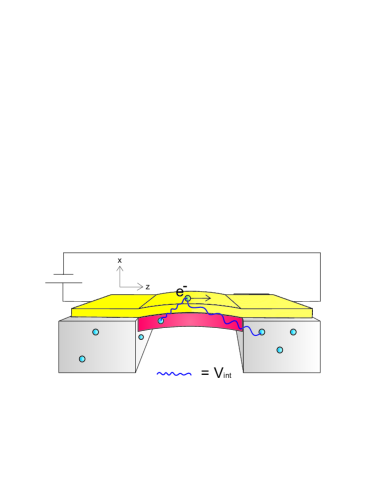
Figure 6: (Color online)Sketch of the distribution of charges in the device. When the system oscillates, these charges induce time dependent potentials which create electron-hole pairs in the metallic layer deposited on top of the beam, absorbing part of the mechanical energy of the flexural mode. See text for details.

VIII Dissipation in a metallic conductor

Many of the current realizations of nanomechanical devices monitor the system by means of currents applied through metallic conductors attached to the oscillators. The vibrations of the device couple to the electrons in the metallic part. This coupling is useful in order to drive and measure the oscillations, but it can also be a source of dissipation. We will apply here the techniques described in   Guinea et al. (2004); Guinea (2005) (see also   White Jr. and Pohl (1995)) in order to analyze the energy loss processes due to the excitations in the conductor.

We assume that the leading perturbation acting on the electrons in the metal are offset charges randomly distributed throughout the device. A charge $q$ at position ${\bf\vec{R}}$ interacts with an energy

$$V({\bf\vec{r}},t)\equiv\frac{q^{2}}{\epsilon_{0}|{\bf\vec{R}}(t)-{\bf\vec{r}}(t)|}$$ (22)

with another charge $q$ at a position ${\bf\vec{r}}$ inside the metal, see fig.[6]. As the bulk of the device is an insulator, this potential is only screened by a finite dielectric constant, $\epsilon_{0}$. The oscillations of the system at frequency $\omega_{0}$ modulate the relative distance $|{\bf\vec{R}}(t)-{\bf\vec{r}}(t)|$, leading to a time dependent potential acting on the electrons of the metal.

The probability per unit time of absorbing a quantum of energy $\omega_{0}$ can be written, using second order perturbation theory, as   Guinea et al. (2004); Guinea (2005):

$$\Gamma=\int d{\bf\vec{r}}d{\bf\vec{r}}^{\prime}dtdt^{\prime}V({\bf\vec{r}},t)V({\bf\vec{r}}^{\prime},t^{\prime})\rm{Im}\chi[{\bf\vec{r}}-{\bf\vec{r}}^{\prime},t-t^{\prime}]e^{i\omega_{0}(t-t^{\prime})}$$ (23)

where $\rm{Im}\chi[{\bf\vec{r}}-{\bf\vec{r}}^{\prime},t-t^{\prime}]$ is the imaginary part of the response function of the metal.

Charges in the oscillating part of the device. We write the relative distance as ${\bf\vec{R}}(t)-{\bf\vec{r}}(t)={\bf\vec{R}}_{0}-{\bf\vec{r}}_{0}+\delta{\bf\vec{R}}(t)-\delta{\bf\vec{r}}(t)$ and expand $V({\bf\vec{r}},t)$, whose time-dependent part is approximately

$$V({\bf\vec{r}},t)\approx\frac{q^{2}\left[{\bf\vec{R}}_{0}-{\bf\vec{r}}_{0}\right]\cdot\left[\delta{\bf\vec{R}}(t)-\delta{\bf\vec{r}}(t)\right]}{\epsilon_{0}|{\bf\vec{R}}_{0}-{\bf\vec{r}}_{0}|^{3}}$$ (24)

For a flexural mode, we have that $\left[{\bf\vec{R}}_{0}-{\bf\vec{r}}_{0}\right]\cdot[\delta{\bf\vec{R}}(t)-\delta{\bf\vec{r}}(t)]$ has turned into $[X_{0}-x_{0}]\cdot[\delta X(t)-\delta x(t)]\sim t\cdot A\cdot\sin(\omega t)$, where $t=t_{\rm ins}+t_{\rm metal}$ is the thickness of the beam and $A$ is the amplitude of vibration of the mode. Thus the average estimate for this case for the correction of $V({\bf\vec{r}},t)$ is

$$\delta V({\bf\vec{r}},t)\sim\frac{q^{2}}{\epsilon_{0}}\frac{t\cdot A\cdot\sin(\omega t)}{L^{3}}\,\,,$$ (25)

$L$ being the resonator’s length.

The integral over the region occupied by the metal in eq.(23) can be written as an integral over ${\bf\vec{r}}_{0}$ and ${\bf\vec{r}}_{0}^{\prime}$. The dielectric constant of a dirty metal in the Random Phase Approximation is   Nozieres and Pines (1999):

$${\rm Im}\chi({\bf\vec{r}}-{\bf\vec{r}}^{\prime},t-t^{\prime})=\int\frac{d\omega d{\bf\vec{q}}}{(2\pi)^{4}}e^{i{\bf\vec{q}}({\bf\vec{r}}-{\bf\vec{r}}^{\prime})}e^{i\omega(t-t^{\prime})}\frac{|\omega|}{e^{4}D\nu|{\bf\vec{q}}|^{2}}$$ (26)

where $e$ is the electronic charge, $D=\hbar v_{\rm F}l$ is the diffusion constant, $v_{\rm F}$ is the Fermi velocity, $l$ is the mean free path, and $\nu\approx(k_{\rm F}t_{\rm metal})^{2}/(\hbar v_{\rm F})$ is the one dimensional density of states.

Combining eq.(23) and eq.(26), and assuming that the position of the charge, ${\bf\vec{R}}_{0}$ is in a generic point inside the beam, and that the length scales are such that $k_{\rm F}^{-1},t_{\rm metal},t\ll L$, we can obtain the leading dependence of $\Gamma$ in eq.(23) on $L$:

$$\Gamma\approx\frac{|\omega_{0}|A^{2}}{D\nu L}\left(\frac{t}{L}\right)^{2}\approx\frac{|\omega_{0}|A^{2}}{lk_{\rm F}^{2}L^{3}}\left(\frac{t}{t_{\rm metal}}\right)^{2}$$ (27)

where we also assume that $|q|=e$. The energy absorbed per cycle of oscillation and unit volume will be $\Delta E=(2\pi/\omega_{0})\hbar\omega_{0}\Gamma_{\rm ph}/t^{2}L=2\pi\hbar\Gamma_{\rm ph}/t^{2}L$, and the inverse quality factor $Q^{-1}_{\rm ph}(\omega_{0})$ will correspond to

$$Q^{-1}_{\rm ph}(\omega_{0})=\frac{1}{2\pi}\frac{\Delta E}{E_{0}}=\frac{\hbar\Gamma_{\rm ph}}{twL}\frac{1}{\frac{1}{2}\rho\omega_{0}^{2}A^{2}}\,\,,$$ (28)

where $E_{0}$ is the elastic energy stored in the vibration and $A$ the amplitude of vibration. Substituting the result for $\Gamma$ one obtains

$$Q^{-1}\approx\frac{2\hbar}{lk_{\rm F}^{2}L^{4}t^{2}\rho\omega_{0}}\left(\frac{t}{t_{\rm metal}}\right)^{2}$$ (29)

In a narrow metallic wire of width $t_{\rm metal}$, we expect that $l\sim t_{\rm metal}$.

Typical values for the parameters in eq.(29) are $k_{\rm F}^{-1}\approx 1$Å, $A\approx 1$Å, $l\sim t_{\rm metal}\approx 10$nm $\sim 10^{2}$Å, $t\approx 100$nm $\approx 10^{3}$Åand $L\approx 1\mu$m $\approx 10^{4}$Å. Hence, each charge in the device gives a contribution to $Q^{-1}$ of order $10^{-20}$. The effect of all charges is obtained by summing over all charges in the beam. If their density is $n_{q}$, we obtain:

$$Q^{-1}\approx\frac{2\hbar n_{q}}{lk_{\rm F}^{2}L^{3}\rho\omega_{0}}\left(\frac{t}{t_{\rm metal}}\right)^{2}$$ (30)

For reasonable values of the density of charges, $n_{q}=l_{q}^{-3},l_{q}\gtrsim 10$nm, this contribution is negligible, $Q^{-1}\lesssim 10^{-16}$.

Charges in the substrate surrounding the device.Many resonators, however, are suspended, at distances much smaller than $L$, over an insulating substrate, which can also contain unscreened charges. As the Coulomb potential induced by these charges is long range, the analysis described above can be applied to all charges within a distance of order $L$ from the beam. Moreover, the motion of these charges is not correlated with the vibrations of the beam, so that now the value of $\left|\delta{\bf\vec{R}}(t)-\delta{\bf\vec{r}}(t)\right|$ has to be replaced by:

$$\left|\delta{\bf\vec{R}}(t)-\delta{\bf\vec{r}}(t)\right|\approx Ae^{i\omega_{0}t}\,\,,$$ (31)

and the value of $|{\bf\vec{R}}_{0}-{\bf\vec{r}}_{0}|\sim L$. Assuming, as before, a density of charges $n_{q}=l_{q}^{3}$, the effect of all charges in the substrate leads to:

$$Q^{-1}\approx\frac{2\hbar L}{l(k_{\rm F}t_{\rm metal})^{2}l_{q}^{3}t^{2}\rho\omega_{0}}\approx 0.3\frac{\hbar L^{3}}{l(k_{\rm F}t_{\rm metal})^{2}l_{q}^{3}t^{3}\sqrt{E\rho}}\,\,,$$ (32)

where the second result corresponds to the fundamental mode, $\omega_{0}\approx 6.5(t/L^{2})\sqrt{E/\rho}$. For values $L\approx 1\mu$m, $A\approx 1$Å, $k_{\rm F}^{-1}\approx 1$Å, $l\sim t_{\rm metal}\approx 10$nm and $l_{q}\sim 10$nm, we obtain $Q^{-1}\sim 10^{-9}$. Thus, given the values of $Q^{-1}$ reached experimentally until now this mechanism can be disregarded, although it sets a limit to $Q^{-1}$ at the lowest temperatures. It also has to be noted that this estimate neglects cancelation effects between charges of opposite signs.

IX Conclusions

Disorder and configurational rearrangements of atoms and adsorbed impurities at surfaces of nanoresonators dominate dissipation of their vibrational eigenmodes at low temperatures. We have given a theoretical framework to describe in a unified way these processes, improving and extending previous ideas  Seoanez et al. (2007). Based on the good description of low temperature properties of disordered bulk insulators provided by the Standard Tunneling Model   Anderson et al. (1972); Phillips (1972); Esquinazi (1998), and in particular of acoustic phonon attenuation in such systems, we adapt it to describe the damping of 1D flexural and torsional modes of NEMS associated to the amorphous-like nature of their surfaces.

Correcting some aspects of   Seoanez et al. (2007), we have calculated the damping of the modes by the presence of an ensemble of independent Two-Level Systems (TLSs) coupled to the local deformation gradient field $\partial_{i}u_{j}$ created by vibrations. The different dissipation channels to which this ensemble gives rise have been described, focussing the attention on the two most important: relaxation dynamics of biased TLSs and dissipation due to symmetric non-resonant TLSs. The first one is caused by the finite time it takes for the TLSs to readjust their equilibrium populations when their bias $\Delta^{z}_{0}$ is modified by local strains, with biased TLSs playing the main role, as this effect is $\propto[\Delta^{z}_{0}/\sqrt{(\Delta^{z}_{0})^{2}+(\Delta^{x}_{0})^{2}}]^{2}$. In terms of the excitation spectrum of the TLSs, it corresponds to a lorentzian peak around $\omega=0$. The second effect is due to the modified absorption spectrum of the TLSs caused by their coupling to all the vibrations, specially the flexural modes, whose high density of states at low energies leads to subohmic damping  Leggett et al. (1987); Kehrein and Mielke (1996); Weiss (1999). A broad incoherent spectral strength is generated, enabling the ”dressed-by-the-modes” TLSs to absorb energy of an excited mode and deliver it to the rest of the modes when they decay.

We have given analytical expressions for the contributions of these mechanisms to the linewidth of flexural (eqs.(6), (10)) or torsional modes (eqs.(13), (17)) in terms of the inverse quality factor $Q^{-1}(\omega_{0})=\Delta\omega_{0}/\omega_{0}$, showing the dependencies on the dimensions, temperature and other relevant parameters characterizing the device. We have compared the two mechanisms, concluding that relaxation dominates dissipation, with a predicted $Q^{-1}(\omega_{0},T)\sim T^{1/2}/\omega_{0}$ . Expressions have been provided for damping of flexural modes in cantilevers and doubly-clamped beams, as well as for damping of their torsional modes.

Analytical predictions for associated frequency shifts have been also calculated (eq.(21)). Some important successes have been achieved, like the qualitative agreement with a sublinear temperature dependence of $Q^{-1}(T)$, the presence of a peak in the frequency shift temperature dependence $\delta\omega/\omega(T)$, or the observed order of magnitude of $Q^{-1}(T)$ in the existing experiments studying flexural phonon attenuation at low temperatures  Zolfagharkhani et al. (2005b); Shim et al. (2007). Nevertheless, the lack of full quantitative agreement has led to a discussion on the assumptions of the model, its links with the physical processes occurring at the surfaces of NEMS, its range of applicability and improvements to reach the desired quantitative fit.

Finally, we have also considered the contributions to the dissipation due to the presence of metallic electrodes deposited on top of the resonators, which can couple to the electrostatic potential induced by random charges. We have shown that the coupling to charges within the vibrating parts does not contribute appreciably to the dissipation. Coupling to charges in the substrate, although more significant, still leads to small dissipation effects (eq.(32)), imposing a limit at low temperatures $Q^{-1}\sim 10^{-9}$, very small compared to the values reached in current experiments   Zolfagharkhani et al. (2005b); Shim et al. (2007).

X Acknowledgements

C. S. and F. G. acknowledge funding from MEC (Spain) through FPU grant, grant FIS2005-05478-C02-01 and the Comunidad de Madrid, through the program CITECNOMIK, CM2006-S-0505-ESP-0337. A.H.C.N. is supported through NSF grant DMR-0343790.

Appendix A Calculation of the spectral function for the bending modes

The starting point is the Hamiltonian of ref.  Seoanez et al. (2007), $\textsl{H}=\Delta_{0}\sigma_{x}+\gamma\sigma_{z}\partial_{i}u_{j}$, where $\partial_{i}u_{j}$ is a component of the deformation gradient matrix. In the case of the bending modes of a rod of dimensions $L$, $t$ and $w$, and mass density $\rho$, there are two variables $X(z),Y(z)$ (transversal displacements of the rod as a function of the position along its length, z) obeying   Landau and Lifshitz (1959)

$$EI_{y}\frac{\partial^{4}X}{\partial z^{4}} = -\rho tw\frac{\partial^{2}X}{\partial t^{2}}$$

$$EI_{x}\frac{\partial^{4}Y}{\partial z^{4}} = -\rho tw\frac{\partial^{2}Y}{\partial t^{2}}$$ (33)

(where $I_{y}=t^{3}w/12$, and $I_{x}=w^{3}t/12$), so that there are plane waves $X(z,t),Y(z,t)\sim e^{i(kz-\omega t)}$, but with a quadratic dispersion relation, $\omega_{j}(k)=\sqrt{\frac{EI_{j}}{\rho ab}}\times k^{2}$. One can thus express $X(z),Y(z)$ in terms of bosonic operators, for example $X(0)=\sum_{k}\sqrt{\frac{\hbar}{2\rho twL\omega_{k}}}(a_{k}^{{\dagger}}+a_{k})$. We can relate this variables to the strain field $\partial_{i}u_{j}$ through the free energy F:

$$F_{rod}=\frac{1}{2}\int dzEI_{y}\Bigl{(}\frac{\partial^{2}X}{\partial z^{2}}\Bigr{)}^{2}+EI_{x}\Bigl{(}\frac{\partial^{2}Y}{\partial z^{2}}\Bigr{)}^{2}=\frac{1}{2}\int dz\int dS\frac{1}{2}\lambda\sum_{i}u_{ii}^{2}+\mu\sum_{i,k}u_{ik}^{2}\approx\frac{1}{2}\int dz\int dS(\frac{3}{2}\lambda+9\mu)u_{ij}^{2}$$ (34)

extracting an average equivalence for one component $u_{ij}$, $u_{ij}\approx 2\sqrt{EI_{y}/(3\lambda+18\mu)tw}\partial^{2}X/\partial z^{2}$. The interaction term in the Hamiltonian is then

$$H_{int}=\hbar\sigma_{z}\sum_{k}\lambda\frac{k^{2}}{\sqrt{\omega_{k}}}(a^{\dagger}_{k}+a_{k})=\hbar\sigma_{z}\sum_{ij}\sum_{k}\Bigl{[}2\gamma\frac{\Delta_{0}^{x}}{\Delta_{0}}\sqrt{\frac{EI_{y}}{(3\lambda+18\mu)tw}}\sqrt{\frac{1}{2\rho tw\hbar L}}\Bigr{]}\frac{(k^{ij})^{2}}{\sqrt{\omega_{k}^{ij}}}(a_{k}^{ij{\dagger}}+a_{k}^{ij})$$ (35)

So we have approximately 9 times the same Hamiltonian, once for each $u_{ij}$, and the corresponding spectral function $J(\omega)$ will be nine times the one calculated for

$$H_{int}=\hbar\sigma_{z}\sum_{k}\lambda\frac{k^{2}}{\sqrt{\omega_{k}}}(a^{\dagger}_{k}+a_{k})\simeq\hbar\sigma_{z}\sum_{k}\Bigl{[}2\gamma\frac{\Delta_{0}^{x}}{\Delta_{0}}\sqrt{\frac{EI_{y}}{(3\lambda+18\mu)tw}}\sqrt{\frac{1}{2\rho tw\hbar L}}\Bigr{]}\frac{k^{2}}{\sqrt{\omega_{k}}}(a^{\dagger}_{k}+a_{k})$$ (36)

For a Hamiltonian of the class $H=\Delta_{0}\sigma_{x}+\hbar\sigma_{z}\sum_{k}\lambda_{k}(a^{\dagger}_{k}+a_{k})$ the spectral function $J(\omega)$ is given by $J(\omega)=\frac{1}{2\pi}\sum_{k}\lambda_{k}^{2}\delta(\omega-\omega_{k})$, so that in our case the expression for it is

$$J(\omega)=\frac{1}{2\pi}\sum_{k}\Bigl{[}2\gamma\frac{\Delta_{0}^{x}}{\Delta_{0}}\sqrt{\frac{EI_{y}}{(3\lambda+18\mu)tw}}\sqrt{\frac{1}{2\rho tw\hbar L}}\frac{k^{2}}{\sqrt{\omega_{k}}}\Bigr{]}^{2}\delta(\omega-\omega_{k})$$ (37)

Taking the continuum limit ($\frac{1}{L}\sum_{k}\rightarrow\frac{1}{\pi}\int dk$):

$$J(\omega)=\frac{2L}{(2\pi)^{2}}\int_{k_{min}}^{k_{max}}dk\Bigl{[}2\gamma\frac{\Delta_{0}^{x}}{\Delta_{0}}\sqrt{\frac{EI_{y}}{(3\lambda+18\mu)tw}}\sqrt{\frac{1}{2\rho tw\hbar L}}\Bigr{]}^{2}\frac{k^{4}}{\omega_{k}}\delta(\omega-\omega_{k})$$ (38)

Using the dispersion relation $\omega_{j}(k)=\sqrt{\frac{EI_{j}}{\rho ab}}\times k^{2}=c\times k^{2}$ we express the integral in terms of the frequency:

$$J(\omega)=\frac{L}{(2\pi)^{2}}\int_{\omega_{min}}^{\omega_{co}}\frac{d\omega_{k}}{\sqrt{c\,\omega_{k}}}\Bigl{[}2\gamma\frac{\Delta_{0}^{x}}{\Delta_{0}}\sqrt{\frac{EI_{y}}{(3\lambda+18\mu)tw}}\sqrt{\frac{1}{2\rho tw\hbar L}}\Bigr{]}^{2}\frac{k^{4}}{\omega_{k}}\delta(\omega-\omega_{k})=\frac{L}{(2\pi)^{2}}\Bigl{[}2\gamma\frac{\Delta_{0}^{x}}{\Delta_{0}}\sqrt{\frac{EI_{y}}{(3\lambda+18\mu)tw}}\sqrt{\frac{1}{2\rho tw\hbar L}}\Bigr{]}^{2}\frac{\sqrt{\omega}}{c^{5/2}}$$ (39)

$J_{{\rm flex}}(\omega)$ is just 9 times this, eq.(2).

Appendix B Dissipation from off-resonance dressed TLS$\rm{s}$

We follow the method of ref.  Guinea (1985). The form of $A(\omega)$, the spectral function of a single TLS, for frequencies $\omega\ll\Delta$ and $\omega\gg\Delta$ can be estimated using perturbation theory. Without the interaction, the ground state $|s\rangle$ of the TLS is the symmetric combination of the ground states of the two wells, and the excited state is the antisymmetric one, $|a\rangle$. We will use Fermi’s Golden Rule applied to the subohmic spin-boson Hamiltonian, $H=\Delta\sigma_{x}+\hbar\lambda\sigma_{z}\sum_{k}\Bigl{[}\frac{k^{2}}{\sqrt{\omega_{k}}}\Bigr{]}(a^{\dagger}_{k}+a_{k})+\sum_{k}\hbar\omega(k)a_{k}^{{\dagger}}a_{k}$, where $a_{k}$ is the annihilation operator of a bending mode $k$. Considering only the low energy modes $\omega(k)\ll\Delta$, to first order the ground state and a state with energy $\omega(k)$ are given by

$$|g\rangle \simeq |s\rangle-\frac{\frac{\lambda k^{2}}{\sqrt{\omega_{k}}}}{2\Delta}a_{k}^{{\dagger}}|a\rangle+...\hphantom{xx},$$

$$|k\rangle \simeq a_{k}^{{\dagger}}|s\rangle-\frac{\frac{\lambda k^{2}}{\sqrt{\omega_{k}}}}{2\Delta}|a\rangle+...\hphantom{xx}.$$ (40)

We estimate the behavior of $A(\omega)$ by taking the matrix element of $\sigma_{z}$ between these two states, obtaining (remember that $\omega(k)\propto k^{2}$)

$$A(\omega)\sim\frac{\hbar\alpha_{b}\sqrt{\omega_{co}}\sqrt{\omega}}{\Delta^{2}}+...\hphantom{xx},\hphantom{xx}\omega(k)\ll\Delta.$$ (41)

The expression in the numerator is proportional to the spectral function of the coupling, $J(\omega)=\alpha_{b}\sqrt{\omega_{co}}\sqrt{\omega}$. Now we turn our attention to the case $\omega(k)\gg\Delta$, where the ground state $|g\rangle$ and an excited state $|k\rangle$ can be written as

$$|g\rangle \simeq |s\rangle-\frac{\lambda k^{2}/\sqrt{\omega_{k}}}{\hbar\omega_{k}+2\Delta}a_{k}^{{\dagger}}|a\rangle+...\hphantom{xx},$$

$$|k\rangle \simeq a_{k}^{{\dagger}}|s\rangle+\frac{\lambda k^{2}/\sqrt{\omega_{k}}}{\hbar\omega_{k}-2\Delta}|a\rangle+...\hphantom{xx}.$$ (42)

The matrix element $\langle 0|\sigma_{z}|k\rangle$ is $\sim\frac{\lambda k^{2}}{\sqrt{\omega_{k}}}\frac{4\Delta}{(\hbar\omega_{k})^{2}}$, leading to

$$A(\omega)\sim\frac{\alpha_{b}\sqrt{\omega_{co}}\Delta^{2}}{\hbar^{3}\omega^{7/2}}+...\hphantom{xx},\hphantom{xx}\omega(k)\gg\Delta.$$ (43)

B.1 Value of $A_{\rm{off-res}}^{\rm{tot}}(\omega_{0})$

Now we will add the contributions of all the non-resonant TLSs using the probability distribution $P(\Delta^{x}_{0},\Delta^{z}_{0})=P_{0}/\Delta^{x}_{0}$   Anderson et al. (1972); Phillips (1972). For the case of weak coupling, $\alpha_{b}<1/2$ and $\omega_{0}\geq(2\alpha_{b})^{2}\omega_{co}$, which is the one found in experiments, one has

$$A_{\rm{off}}^{\rm{tot}}(\omega_{0})\sim\int_{\hbar[\omega_{0}+\Gamma(\omega_{0})]}^{\varepsilon_{max}} d\Delta^{x}_{0}\int_{-\Delta^{x}_{0}}^{\Delta^{x}_{0}}d\Delta_{z}\frac{P}{\Delta^{x}_{0}}\frac{\hbar\alpha_{b}\sqrt{\omega_{co}}\sqrt{\omega_{0}}}{(\Delta^{x}_{0})^{2}}$$

$$+\int_{\hbar(2\alpha_{b})^{2}\omega_{co}}^{\hbar[\omega_{0}-\Gamma(\omega_{0})]} d\Delta^{x}_{0}\int_{-\Delta^{x}_{0}}^{\Delta^{x}_{0}}d\Delta_{z}\frac{P}{\Delta^{x}_{0}}\frac{\alpha_{b}\sqrt{\omega_{co}}(\Delta^{x}_{0})^{2}}{\hbar^{3}\omega_{0}^{7/2}}$$

obtaining the result $A_{\rm{off-res}}^{\rm{tot}}(\omega_{0})\approx 2P\alpha_{b}\sqrt{\omega_{co}/\omega_{0}}$.

B.2 The off-resonance contribution for T $>$ 0

Using the same scheme, the modifications due to the temperature will appear in the density of states of absorption and emission of energy corresponding to a ”dressed” TLS, $A(\Delta,\omega,T)$. Now there will be a probability for the TLS to be initially in the excited antisymmetric state, $|a\rangle$, proportional to $\exp[-\Delta/kT]$, and to emit energy $\hbar\omega$ giving it to our externally excited mode, $|k,n\rangle$, thus compensating the absorption of energy corresponding to the opposite case (transition from $|s\rangle|k,n\rangle$ to $|a\rangle|k,n-1\rangle$), but contributing in an additive manner to the total amount of fluctuations, which are the ones defining the linewidth of the vibrational mode observed in experiments, fixing the value of $Q^{-1}(\omega,T)$. The expression for $A(\Delta,\omega,T)$ is given by

$$A(\omega,T)=\frac{1}{Z}\sum_{i}\sum_{f}|\langle i|\sigma_{z}|f\rangle|^{2}e^{-\frac{E_{i}}{kT}}\delta[\hbar\omega-(E_{f}-E_{i})]$$ (44)

We consider a generic state $|i_{a}\rangle=|a\rangle|k_{1}n_{1},...,k_{j}n_{j},...\rangle$ or $|i_{s}\rangle=|s\rangle|k_{1}n_{1},...,k_{j}n_{j},...\rangle$, and states that differ from it in $\hbar\omega_{j}$, $|f_{a\pm}\rangle=|a\rangle|k_{1}n_{1},...,k_{j}n_{j}\pm 1,...\rangle$ and $|f_{s\pm}\rangle|s\rangle|k_{1}n_{1},...,k_{j}n_{j}\pm 1,...\rangle$. As for $T=0$, we will correct them to first order in the interaction Hamiltonian $H_{int}=\hbar\lambda\sigma_{z}\sum_{k}\sqrt{\omega_{k}}(a^{\dagger}_{k}+a_{k})$, and then calculate the square of the matrix element of $\sigma_{z}$, $|\langle i|\sigma_{z}|f\rangle|^{2}$.

Elements $|\langle i_{a,s}|\sigma_{z}|f_{a+,s+}\rangle|^{2}$ correspond to absorption by the ”dressed” TLS of an energy $\hbar\omega_{j}$ from the mode $k_{j}$, while elements $|\langle i_{a,s}|\sigma_{z}|f_{a-,s-}\rangle|^{2}$ correspond to emission and ”feeding” of the mode with a phonon $\hbar\omega_{j}$. The expressions for the initial states are

$$|i_{s}\rangle=|s\rangle|k_{1}n_{1},...,k_{j}n_{j},...\rangle \rightarrow |s\rangle|k_{1}n_{1},...,k_{j}n_{j},...\rangle+\sum_{k_{i}\ni n_{i}>0}\frac{\hbar\lambda\sqrt{n_{i}\omega_{i}}}{\hbar\omega_{i}+2\Delta}|a\rangle|...k_{i}n_{i}-1...\rangle$$

$$- \sum_{\forall k_{i}}\frac{\hbar\lambda\sqrt{(n_{i}+1)\omega_{i}}}{\hbar\omega_{i}-2\Delta}|a\rangle|...k_{i}n_{i}+1...\rangle$$

$$|i_{a}\rangle=|a\rangle|k_{1}n_{1},...,k_{j}n_{j},...\rangle \rightarrow |a\rangle|k_{1}n_{1},...,k_{j}n_{j},...\rangle+\sum_{k_{i}\ni n_{i}>0}\frac{\hbar\lambda\sqrt{n_{i}\omega_{i}}}{\hbar\omega_{i}-2\Delta}|s\rangle|...k_{i}n_{i}-1...\rangle$$ (45)

$$- \sum_{\forall k_{i}}\frac{\hbar\lambda\sqrt{(n_{i}+1)\omega_{i}}}{\hbar\omega_{i}+2\Delta}|s\rangle|...k_{i}n_{i}+1...\rangle$$

and, for example, the state $|f_{a+}\rangle$ is given by

$$|f_{a+}\rangle=|a\rangle|k_{1}n_{1},...,k_{j}n_{j}+1,...\rangle \rightarrow |a\rangle|k_{1}n_{1},...,k_{j}n_{j}+1,...\rangle+\sum_{k_{i}\ni n_{i}>0,i\neq j}\frac{\hbar\lambda\sqrt{n_{i}\omega_{i}}}{\hbar\omega_{i}-2\Delta}|s\rangle|...k_{i}n_{i}-1...k_{j}n_{j}+1...\rangle$$ (46)

$$+ \frac{\hbar\lambda\sqrt{(n_{j}+1)\omega_{j}}}{\hbar\omega_{j}-2\Delta}|s\rangle|...k_{j}n_{j}...\rangle-\sum_{\forall k_{i},i\neq j}\frac{\hbar\lambda\sqrt{(n_{i}+1)\omega_{i}}}{\hbar\omega_{i}+2\Delta}|s\rangle|...k_{i}n_{i}+1...k_{j}n_{j}+1...\rangle$$

$$- \frac{\hbar\lambda\sqrt{(n_{j}+2)\omega_{j}}}{\hbar\omega_{j}+2\Delta}|s\rangle|...k_{j}n_{j}+2...\rangle$$

with similar expression for the rest of states. The value of $|\langle i_{a,s}|\sigma_{z}|f_{a+,s+}\rangle|$ (absorption) is $|\langle i_{a,s}|\sigma_{z}|f_{a+,s+}\rangle|=\Bigl{|}\frac{\lambda\sqrt{(n_{j}+1)\omega_{j}}4\Delta}{(\hbar\omega_{j})^{2}-4\Delta^{2}}\Bigr{|}$ , with $n_{j}=0,1,...$, while for emission the result is $|\langle i_{a,s}|\sigma_{z}|f_{a-,s-}\rangle|=\Bigl{|}\frac{\lambda\sqrt{n_{j}\omega_{j}}4\Delta}{(\hbar\omega_{j})^{2}-4\Delta^{2}}\Bigr{|}$, with $n_{j}=1,...$. Taking the limits we considered at T = 0 ($\hbar\omega_{j}\ll\Delta$ and $\hbar\omega_{j}\gg\Delta$) the results are the same as for T = 0 for absorption, except for a factor $(n_{j}+1)$, and we also have now the possibility of emission, with the same matrix element but with the factor $n_{j}$:

$$\rm{Absorption} \left\{\begin{array}[]{ll}\sim\frac{(n_{j}+1)\hbar\alpha_{b}\sqrt{\omega_{co}}\sqrt{\omega}}{\Delta^{2}}&\hbar\omega_{j}\ll\Delta\\ \sim\frac{(n_{j}+1)\alpha_{b}\sqrt{\omega_{co}}\Delta^{2}}{\hbar^{3}\omega^{7/2}},&\hbar\omega_{j}\gg\Delta\end{array}\right.$$ (49)

$$\rm{Emission} \left\{\begin{array}[]{ll}\sim\frac{n_{j}\hbar\alpha_{b}\sqrt{\omega_{co}}\sqrt{\omega}}{\Delta^{2}}&\hbar\omega_{j}\ll\Delta\\ \sim\frac{n_{j}\alpha_{b}\sqrt{\omega_{co}}\Delta^{2}}{\hbar^{3}\omega^{7/2}},&\hbar\omega_{j}\gg\Delta\end{array}\right.$$ (52)

Now we have to sum over all initial states, and noting that the first order correction to the energy of any eigenstate is 0, the partition function, Z, is easy to calculate, everything factorizes, and the result is, for example in the case $\hbar\omega_{j}\ll\Delta$:

$$A_{abs}(\Delta,\omega_{j},T)=\frac{1}{Z}\sum_{i\neq j,n_{i}=0}^{\infty}\sum_{n_{j}=0}^{\infty}\frac{\hbar\alpha_{b}\sqrt{\omega_{co}}\sqrt{\omega_{j}}}{\Delta^{2}}(n_{j}+1)e^{-\frac{\hbar\omega_{j}n_{j}}{kT}}e^{-\frac{\hbar\sum_{i}n_{i}\omega_{i}}{kT}}=\frac{\hbar\alpha_{b}\sqrt{\omega_{co}}}{\Delta^{2}}\frac{\sqrt{\omega_{j}}}{1-e^{-\frac{\hbar\omega_{j}}{kT}}}$$

$$A_{em}(\Delta,-\omega_{j},T)=\frac{1}{Z}\sum_{i\neq j,n_{i}=0}^{\infty}\sum_{n_{j}=1}^{\infty}\frac{\hbar\alpha_{b}\sqrt{\omega_{co}}\sqrt{\omega_{j}}}{\Delta^{2}}n_{j}e^{-\frac{\hbar\omega_{j}n_{j}}{kT}}e^{-\frac{\hbar\sum_{i}n_{i}\omega_{i}}{kT}}=\frac{\hbar\alpha_{b}\sqrt{\omega_{co}}}{\Delta^{2}}\frac{\sqrt{\omega_{j}}e^{-\frac{\hbar\omega_{j}}{kT}}}{1-e^{-\frac{\hbar\omega_{j}}{kT}}}$$ (53)

In $A_{abs}(\Delta,\omega_{j},T)$ we have added the contributions from the matrix elements $|\langle i_{s}|\sigma_{z}|f_{s+}\rangle|^{2}e^{\frac{\Delta}{kT}}+|\langle i_{a}|\sigma_{z}|f_{a+}\rangle|^{2}e^{\frac{-\Delta}{kT}}=|\langle i_{s}|\sigma_{z}|f_{s+}\rangle|^{2}[e^{\frac{\Delta}{kT}}+e^{\frac{-\Delta}{kT}}]$ . The sum of exponentials cancels with the partition function of the TLS (appearing as a factor in the total Z), leading in this way to the expression above (the same applies for $A_{em}(\Delta,-\omega_{j},T)$). The total fluctuations will be proportional to their sum, which thus turns out to be at this level of approximation $\propto\rm{cotanh}[\hbar\omega_{j}/kT]$:

$$A_{diss}(\Delta,\omega_{j},T)=A_{abs}(\Delta,\omega_{j},T)+A_{em}(\Delta,-\omega_{j},T)=A_{diss}(\Delta,\omega_{j},T=0)\rm{cotanh}\Bigl{[}\frac{\hbar\omega_{j}}{kT}\Bigr{]}$$ (54)

In fact, this result applies for any other type of modes, independently of its dispersion relation, provided the coupling Hamiltonian is linear in $\sigma_{z}$ and $(a_{-k}^{\dagger}+a_{k})$ and everything is treated at this level of perturbation theory. Moreover, it can be proven that if one has an externally excited mode with an average population $\langle n_{j}\rangle$ , and fluctuations around that value are thermal-like, with a probability $\propto\exp[-|n_{j}-\langle n_{j}\rangle|/kT)]$, one recovers again the same temperature dependence, $\propto\rm{cotanh}[\hbar\omega_{j}/kT]$.

Appendix C Derivation of $Q^{-1}_{\rm{rel}}(\omega_{0},T)$, eq.(10)

As discussed after eq.(9), we have to sum over underdamped TLSs, $\varepsilon\geq[30\alpha_{b}\sqrt{\omega_{co}}T]^{2/3}$, using the approximation for $\Gamma$, $\Gamma(\varepsilon,T)\sim 30\alpha_{b}\sqrt{\omega_{co}}T/\sqrt{\varepsilon}$. Moreover, if $\omega_{0}\geq\Gamma(\varepsilon=[30\alpha_{b}\sqrt{\omega_{co}}T]^{2/3},T)$ then in the whole integration range $\omega_{0}\gg\Gamma(\varepsilon,T)\Leftrightarrow\omega_{0}\tau(\varepsilon,T)\gg 1$ (see fig.(7), so that $\omega_{0}\tau/[1+(\omega_{0}\tau)^{2}]\approx 1/(\omega_{0}\tau)$, see fig.(7). $Q^{-1}_{\rm{rel}}(\omega_{0},T)$ follows:

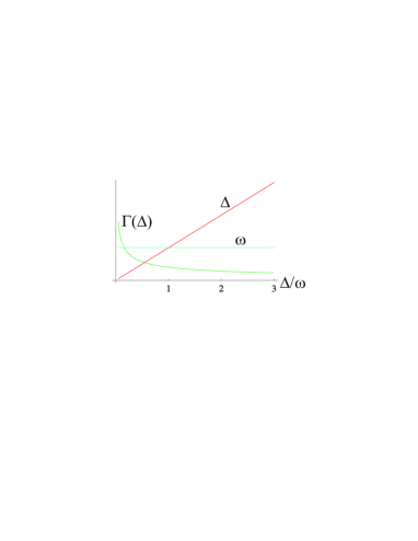
Figure 7: (Color online) Evolution with $\Delta_{r}$ of the different quantities determining the approximations to be taken in the integrand $\omega_{0}\tau/[1+(\omega_{0}\tau)^{2}]$ of eq.(9).

$$Q^{-1}_{\rm{rel}}(\omega_{0},T) \approx \frac{P_{0}\gamma^{2}}{ET}\int_{[30\alpha_{b}\sqrt{\omega_{co}}T]^{2/3}}^{T}d\varepsilon\int_{u_{min}}^{1}du\times$$ (55)

$$\times \frac{\sqrt{1-u^{2}}}{u}\frac{\Gamma(\varepsilon,T)}{\omega_{0}}$$

For temperatures $T\gg[30\alpha_{b}\sqrt{\omega_{co}}T]^{2/3}$, which holds for reasonable T and sizes, the integral, which renders a result of the kind $Q^{-1}_{\rm{rel}}(\omega_{0},T)\approx(1/\omega_{0})(A\sqrt{T}-BT^{1/3})$, can be approximated by just the first term, obtaining eq.(10). In any case for completeness we give the expression for B:

$$B\approx\frac{500P_{0}\gamma^{14/3}}{t^{2}w^{4/3}}\frac{(1+\nu)^{4/3}(1-2\nu)^{4/3}}{E^{11/3}(3-5\nu)}\Bigl{(}\frac{\rho}{E}\Bigr{)}^{1/3}$$ (56)

Also for completeness we give the result for higher temperatures, although for current sizes the condition $\Gamma(\varepsilon=[30\alpha_{b}\sqrt{\omega_{co}}T]^{2/3},T)>\omega_{0}$ implies values of T above the range of applicability of the Standard Tunneling Model. Now for some range of energies $\Gamma(\varepsilon,T)>\omega_{0}$, and the range of integration is divided into two regions, one where $\omega_{0}\tau\gg 1$ and one where the opposite holds:

$$Q^{-1}_{\rm{rel}}(\omega_{0},T)=\frac{P_{0}\gamma^{2}}{ET}\int_{u_{min}}^{1}du\frac{\sqrt{1-u^{2}}}{u}\Bigl{\{}\int_{[30\alpha_{b}\sqrt{\omega_{co}}T]^{2/3}}^{[16\alpha_{b}\sqrt{\omega_{co}}2T/\sqrt{\omega_{0}}]^{2}}dE\,\,\omega_{0}\tau(\varepsilon,T)+\int_{[16\alpha_{b}\sqrt{\omega_{co}}2T/\sqrt{\omega_{0}}]^{2}}^{T}dE\frac{1}{\omega_{0}\tau(\varepsilon,T)}\Bigr{\}}$$ (57)

The final result is $Q^{-1}_{\rm{rel}}(\omega_{0},T)\approx-7P_{0}\gamma^{2}\omega_{0}/T+A\sqrt{T}/\omega_{0}-CT/\omega_{0}^{2}$, with $A$ defined by eq.(10) and C by:

$$C\approx\frac{1500P_{0}\gamma^{6}}{t^{3}w^{2}}\frac{(1+\nu)^{2}(1-2\nu)^{2}}{E^{3}(3-5\nu)^{2}}\Bigl{(}\frac{\rho}{E}\Bigr{)}^{1/2}$$ (58)

All the results for $Q^{-1}_{\rm{rel}}(\omega_{0},T)$ have to be multiplied by the fraction of volume of the resonator presenting amorphous features, $V_{amorph}/(twL)$.

Appendix D Derivation of eqs.(14)-(15)

To derive the interaction Hamiltonian, eq.(14), note that in terms of the deformation gradient matrix $\partial_{i}u_{j}$ it must be $H_{\rm{int}}=\gamma\sigma_{z}\partial_{i}u_{j}$, where the deformations are caused in this case by twisting of the resonator about its main axis. The twisting modes correspond   Landau and Lifshitz (1959) to the rotation angle around the longest main axis $\phi$ obeying the wave equation

$$C\frac{\partial^{2}\phi}{\partial z^{2}}=\rho I\frac{\partial^{2}\phi}{\partial t^{2}}$$ (59)

so the variable $\phi$ can be expressed in terms of boson operators

$$\phi(0) = \sum_{k}\sqrt{\frac{\hbar}{2\rho twL\omega_{k}}}(a_{k}^{{\dagger}}+a_{k})\,,$$

$$\partial\phi\mid_{z=0} = \sqrt{\frac{\hbar}{2\rho twL}}\sum_{k}\frac{k}{\sqrt{\omega_{k}}}(a_{k}^{{\dagger}}+a_{k})$$ (60)

To obtain in terms of the modes’ operators $a_{k}$ an approximate expression for $\partial_{i}u_{j}$, we relate $\partial u$ to $\partial\phi$ through the expressions for the free energy of the rod in terms of both variables,

$$F_{rod}=\frac{1}{2}\int dzC\left(\frac{\partial\phi}{\partial z}\right)^{2}=\frac{1}{2}\int dz\int dS4\mu\left[\left(\frac{\partial u_{x}}{\partial z}\right)^{2}+\left(\frac{\partial u_{y}}{\partial z}\right)^{2}\right]\approx\frac{1}{2}\int dz\int dS8\mu\left(\frac{\partial u_{x}}{\partial z}\right)^{2}$$ (61)

and the approximate relation $\partial u\mid_{z=0}=\partial u_{x}/\partial z=\sqrt{C/(8\mu tw)}\partial\phi\mid_{z=0}$ is found. This relation together with eq.(D) lead to the stated result, eq.(14).

Calculation of E₀.To calculate classically the energy stored of a torsional mode $\phi_{j}(z,t)=A\sin[(2j-1)\pi z/(2L)]\sin(\omega_{j}t)$ we just calculate the kinetic energy in a moment where the elastic energy is zero, for example at time $t=0$. If an element of mass is originally at position $(x,y,z)$ ($x,y$ transversal coordinates), with a torsion $\phi(z,t)$ it moves to

$$\vec{r}(t)=\Bigl{(}\sqrt{x^{2}+y^{2}}\cdot\cos\Bigl{[}\arccos\frac{x}{\sqrt{x^{2}+y^{2}}}+\phi\Bigr{]},\sqrt{x^{2}+y^{2}}\cdot\sin\Bigl{[}\arccos\frac{x}{\sqrt{x^{2}+y^{2}}}+\phi\Bigr{]},z\Bigr{)}$$ (62)

The kinetic energy at time $t=0$ is

$$E_{0}=\int_{0}^{L}dz\int_{-t/2}^{t/2}dx\int_{-w/2}^{w/2}dy\cdot\frac{1}{2}\rho\Bigl{|}\frac{d\overrightarrow{r}}{dt}\Bigr{|}^{2}_{t=0}$$ (63)

Substituting the expression for $\vec{r}(t)$ in the integrand, one arrives at

$$E_{0}=\int_{0}^{L}dz\int_{-t/2}^{t/2}dx\int_{-w/2}^{w/2}dy\cdot\frac{1}{2}\rho A^{2}\omega_{j}^{2}\sin^{2}\Bigl{[}\frac{(2j-1)\pi}{2L}z\Bigr{]}(x^{2}+y^{2})=\frac{1}{48}A^{2}\omega_{j}^{2}\rho L(t^{3}w+w^{3}t)$$ (64)

In terms of the creation and annihilation operators $\phi_{j}(z,t)=\frac{\hbar}{2L\rho I\omega_{j}}(a_{j}^{{\dagger}}+a_{j})e^{i(k_{j}z-\omega t)}$, so the mean square of its amplitude is $\langle\phi_{j}^{2}\rangle=A^{2}/2=\hbar(2n+1)/[2L\rho I\omega_{j}]$. Substituting this in eq.(64) the eq.(15) for $E_{0}$ is obtained.

References

- Seoanez et al. (2007) C. Seoanez, F. Guinea, and A. H. Castro Neto, Europhys. Lett. 78, 60002 (2007).
- Sze (1981) S. Sze, Physics of semiconductor devices (Wiley-Interscience (New York), 1981).
- Craighead (2000) H. G. Craighead, Science 250, 1532 (2000).
- Cleland (2002) A. N. Cleland, Foundations of Nanomechanics (Springer (Berlin), 2002).
- Blencowe (2004) M. Blencowe, Phys. Rep. 395, 159 (2004).
- Ekinci and Roukes (2005) K. L. Ekinci and M. L. Roukes, Rev. Sci. Inst. 76, 061101 (2005).
- Scheible and Blick (2004) D. V. Scheible and R. H. Blick, Appl. Phys. Lett. 84, 4632 (2004).
- Rugar et al. (2004) D. Rugar, R. Budakian, H. Mamin, and B. Chui, Nature 430, 329 (2004).
- Mamin and Rugar (2001) H. J. Mamin and D. Rugar, Appl. Phys. Lett. 79, 3358 (2001).
- K. L. Ekinci and Roukes (2004) X. M. H. H. K. L. Ekinci and M. L. Roukes, Appl. Phys. Lett. 84, 4469 (2004).
- Hopcroft et al. (2007) M. A. Hopcroft, B. Kim, S. Chandorkar, R. Melamud, M. Agarwal, C. M. Jha, G. Bahl, J. Salvia, H. Mehta, H. K. Lee, et al., Appl. Phys. Lett. 91, 013505 (2007).
- Dorignac et al. (2006) J. Dorignac, A. Kalinowski, S. Erramilli, and P. Mohanty, Phys. Rev. Lett. 96, 186105 (2006).
- LaHaye et al. (2004) M. D. LaHaye, O. Buu, B. Camarota, and K. C. Schwab, Science 304, 74 (2004).
- Zolfagharkhani et al. (2005a) G. Zolfagharkhani, A. Gaidarzhy, R. L. Badzey, and P. Mohanty, Phys. Rev. Lett. 94, 030402 (2005a).
- Naik et al. (2006) A. Naik, O. Buu, M. D. LaHaye, A. D. Armour, A. A. Clerk, M. P. Blencowe, and K. C. Schwab, Nature 443, 193 (2006).
- Santamore et al. (2004) D. H. Santamore, A. C. Doherty, and M. C. Cross, Phys. Rev. B 70, 144301 (2004).
- Martin and Zurek (2007) I. Martin and W. H. Zurek, Phys. Rev. Lett. 98, 120401 (2007).
- Jacobs et al. (2007) K. Jacobs, P. Lougovski, and M. Blencowe, Phys. Rev. Lett. 98, 147201 (2007).
- Wei et al. (2006) L. F. Wei, Y. xi Liu, C. P. Sun, and F. Nori, Phys. Rev. Lett. 97, 237201 (2006).
- Thompson et al. (2007) J. D. Thompson, B. M. Zwickl, A. M. Jayich, F. Marquardt, S. M. Girvin, and J. G. E. Harris (2007), eprint arXiv:0707.1724.
- Katz et al. (2007) I. Katz, A. Retzker, R. Straub, and R. Lifshitz, Phys. Rev. Lett. 99, 040404 (2007).
- Cleland and Roukes (1999) A. N. Cleland and M. L. Roukes, Sens. Actuators A 72, 256 (1999).
- Yasumura et al. (2000) K. Y. Yasumura, T. D. Stowe, E. M. Chow, T. Pfafman, T. W. Kenny, B. C. Stipe, and D. Rugar, J. Microelectromech. Syst. 9, 117 (2000).
- Evoy et al. (2000) S. Evoy, A. Olkhovets, L. Sekaric, J. M. Parpia, H. G. Craighead, and D. W. Carr, Appl. Phys. Lett. 77, 2397 (2000).
- Cleland and Roukes (2002) A. N. Cleland and M. L. Roukes, J. Appl. Phys. 92, 2758 (2002).
- Yang et al. (2002) J. L. Yang, T. Ono, and M. Esashi, J. Microelectromech. Syst. 11, 775 (2002).
- Mohanty et al. (2002) P. Mohanty, D. A. Harrington, K. L. Ekinci, Y. T. Yang, M. J. Murphy, and M. L. Roukes, Phys. Rev. B 66, 085416 (2002).
- Ahn and Mohanty (2003) K.-H. Ahn and P. Mohanty, Phys. Rev. Lett. 90, 085504 (2003).
- Husain et al. (2003) A. Husain, J. Hone, H. W. C. Postma, X. M. H. Huang, T. Drake, M. Barbic, A. Scherer, and M. L. Roukes, Appl. Phys. Lett. 83, 1240 (2003).
- Zolfagharkhani et al. (2005b) G. Zolfagharkhani, A. Gaidarzhy, S.-B. Shim, R. Badzey, and P. Mohanty, Phys. Rev. B 72, 224101 (2005b).
- Feng et al. (2006) X. L. Feng, C. A. Zorman, M. Mehregany, and M. L. Roukes (2006), eprint cond-mat/0606711.
- Shim et al. (2007) S.-B. Shim, J. S. Chun, S. W. Kang, S. W. Cho, S. W. Cho, Y. D. Park, P. Mohanty, N. Kim, and J. Kim, Appl. Phys. Lett. 91, 133505 (2007).
- Jimbo and Itao (1968) Y. Jimbo and K. Itao, J. Horological Inst. Jpn. 47, 1 (1968).
- Photiadis and Judge (2004) D. M. Photiadis and J. A. Judge, Applied Physics Letters 85, 482 (2004).
- Zener (1938) C. Zener, Phys. Rev. 53, 90 (1938).
- Lifshitz and Roukes (2000) R. Lifshitz and M. Roukes, Phys. Rev. B 61, 5600 (2000).
- De and Aluru (2006) S. K. De and N. R. Aluru, Phys. Rev. B 74, 144305 (2006).
- Yang et al. (2000) J. Yang, T. Ono, and M. Esashi, Appl. Phys. Lett. 77, 3860 (2000).
- Liu et al. (2005) X. Liu, J. F. Vignola, H. J. Simpson, B. R. Lemon, B. H. Houston, and D. M. Photiadis, J. Appl. Phys. 97, 023524 (2005).
- Chu et al. (2007) M. Chu, R. E. Rudd, and M. P. Blencowe (2007), eprint cond-mat/0705.0015.
- Wang et al. (2004) D. Wang, T. Ono, and M. Esashi, Nanotechnology 15, 1851 (2004).
- Liu et al. (1999) X. Liu, E. J. Thompson, B. E. White Jr., and R. O. Pohl, Phys. Rev. B 59, 11767 (1999).
- Anderson et al. (1972) P. Anderson, B. Halperin, and C. Varma, Philos. Mag. 25, 1 (1972).
- Phillips (1972) W. Phillips, J. Low Temp. Phys. 7, 351 (1972).
- Phillips (1987) W. A. Phillips, Rep. Prog. Phys. 50, 1657 (1987).
- Esquinazi (1998) P. Esquinazi, ed., Tunneling Systems in Amorphous and Crystalline Solids (Springer (Berlin), 1998).
- Yu and Leggett (1988) C. C. Yu and A. J. Leggett, Comm. Cond. Mat. Phys. 14, 231 (1988).
- Esquinazi et al. (2004) P. Esquinazi, M. A. Ramos, and R. König, J. Low Temp. Phys. 135, 27 (2004).
- Shytov et al. (2002) A. V. Shytov, L. S. Levitov, and C. W. J. Beenakker, Phys. Rev. Lett. 88, 228303 (2002).
- Anderson (1986) A. Anderson, J. Non-Crys. Solids 85, 211 (1986).
- Landau and Lifshitz (1959) L. D. Landau and E. M. Lifshitz, Theory of Elasticity (Pergamon Press (London), 1959).
- Arnold et al. (1974) W. Arnold, S. Hunklinger, S. Stein, and K. Dransfeld, J. Non Cryst. Sol. 14, 192 (1974).
- Jäckle (1972) J. Jäckle, Z. Physik 257, 212 (1972).
- Mukhopadhyay et al. (2005) R. Mukhopadhyay, V. V. Sumbayev, M. Lorentzen, J. Kjems, P. A. Andreasen, and F. Besenbacher, Nano Lett. 5, 2385 (2005).
- Sharos et al. (2004) L. Sharos, A. Raman, S. Crittenden, and R. Reifenberger, Appl. Phys. Lett. 84, 4638 (2004).
- Phillips (1988) W. Phillips, Phys. Rev. Lett. 61, 2632 (1988).
- Black and Halperin (1977) J. Black and B. Halperin, Phys. Rev. B 16, 2879 (1977).
- Guinea et al. (2004) F. Guinea, R. A. Jalabert, and F. Sols, Phys. Rev. B 70, 085310 (2004).
- Guinea (2005) F. Guinea, Phys. Rev. B 71, 045424 (2005).
- White Jr. and Pohl (1995) B. E. White Jr. and R. O. Pohl, in Mat. Res. Soc. Symp. (1995), vol. 356, p. 567.
- Nozieres and Pines (1999) P. Nozieres and D. Pines, The Theory of Quantum Liquids (Third Edition) (Perseus Books (Cambridge, Massachusets), 1999).
- Leggett et al. (1987) A. J. Leggett, S. Chakravarty, A. T. Dorsey, M. P. A. Fisher, A. Garg, and W. Zwerger, Rev. Mod. Phys. 59, 1 (1987).
- Kehrein and Mielke (1996) S. Kehrein and A. Mielke, Phys. Lett. A 219, 313 (1996).
- Weiss (1999) U. Weiss, Quantum Dissipative Systems (World Scientific (Singapore), 1999).
- Guinea (1985) F. Guinea, Phys. Rev. B 32, 4486 (1985).