From Discrete Space-Time to Minkowski Space: Basic Mechanisms, Methods and Perspectives

Abstract

This survey article reviews recent results on fermion system in discrete space-time and corresponding systems in Minkowski space. After a basic introduction to the discrete setting, we explain a mechanism of spontaneous symmetry breaking which leads to the emergence of a discrete causal structure. As methods to study the transition between discrete space-time and Minkowski space, we describe a lattice model for a static and isotropic space-time, outline the analysis of regularization tails of vacuum Dirac sea configurations, and introduce a Lorentz invariant action for the masses of the Dirac seas. We mention the method of the continuum limit, which allows to analyze interacting systems. Open problems are discussed.

1 Introduction

It is generally believed that the concept of a space-time continuum (like Minkowski space or a Lorentzian manifold) should be modified for distances as small as the Planck length. The principle of the fermionic projector [4] proposes a new model of space-time, which should be valid down to the Planck scale. This model is introduced as a system of quantum mechanical wave functions defined on a finite number of space-time points and is referred to as a fermion system in discrete space-time. The interaction is described via a variational principle where we minimize an action defined for the ensemble of wave functions. A-priori, there are no relations between the space-time points; in particular, there is no nearest-neighbor relation and no notion of causality. The idea is that these additional structures should be generated spontaneously. More precisely, in order to minimize the action, the wave functions form specific configurations; this can be visualized as a “self-organization” of the particles. As a consequence of this self-organization, the wave functions induce non-trivial relations between the space-time points. We thus obtain additional structures in space-time, and it is conjectured that, in a suitable limit where the number of particles and space-time points tends to infinity, these structures should give rise to the local and causal structure of Minkowski space. In this limit, the configuration of the wave functions should go over to a Dirac sea structure.

This conjecture has not yet been proved, but recent results give a detailed picture of the connection between discrete space-time and Minkowski space. Also, mathematical methods were developed to shed light on particular aspects of the problem. In this survey article we report on the present status, explain basic mechanisms and outline the analytical methods used so far. The presentation is self-contained and non-technical. The paper concludes with a discussion of open problems.

2 Fermion Systems in Discrete Space-Time

We begin with the basic definitions in the discrete setting (for more details see [5]). Let $(H,\mbox{$<\!\!$ \nolinebreak}.|.\mbox{\nolinebreak$>$})$ be a finite-dimensional complex inner product space. Thus $\mbox{$<\!\!$ \nolinebreak}.|.\mbox{\nolinebreak$>$}$ is linear in its second and anti-linear in its first argument, and it is symmetric,

$$\overline{\mbox{$<\!\!$ \nolinebreak}\Psi\>|\>\Phi\mbox{\nolinebreak$>$}}\;=\;\mbox{$<\!\!$ \nolinebreak}\Phi\>|\>\Psi\mbox{\nolinebreak$>$}\quad\;\;\;\;\;\;\;\;\;\;{\mbox{for all~{}$\Psi,\Phi\in H$}}\,,$$

and non-degenerate,

$$\mbox{$<\!\!$ \nolinebreak}\Psi\>|\>\Phi\mbox{\nolinebreak$>$}\;=\;0\;\;\;{\mbox{for all $\Phi\in H$}}\quad\Longrightarrow\quad\Psi\;=\;0\>.$$

In contrast to a scalar product, $\mbox{$<\!\!$ \nolinebreak}.|.\mbox{\nolinebreak$>$}$ need not be positive.

A projector $A$ in $H$ is defined just as in Hilbert spaces as a linear operator which is idempotent and self-adjoint,

$$A^{2}=A\;\;\;\;\;\;\;\;\;\;{\mbox{and}}\;\;\;\;\;\;\;\;\;\;\mbox{$<\!\!$ \nolinebreak}A\Psi\>|\>\Phi\mbox{\nolinebreak$>$}=\mbox{$<\!\!$ \nolinebreak}\Psi\>|\>A\Phi\mbox{\nolinebreak$>$}\quad{\mbox{for all $\Psi,\Phi\in H$}}\>.$$

Let $M$ be a finite set. To every point $x\in M$ we associate a projector $E_{x}$. We assume that these projectors are orthogonal and complete in the sense that

$$E_{x}\>E_{y}\;=\;\delta_{xy}\>E_{x}\;\;\;\;\;\;\;\;\;\;{\mbox{and}}\;\;\;\;\;\;\;\;\;\;\sum_{x\in M}E_{x}\;=\;\mbox{\rm 1 1}\>.$$ (1)

Furthermore, we assume that the images $E_{x}(H)\subset H$ of these projectors are non-degenerate subspaces of $H$, which all have the same signature $(n,n)$. We refer to $n$ as the spin dimension. The points $x\in M$ are called discrete space-time points, and the corresponding projectors $E_{x}$ are the space-time projectors. The structure $(H,\mbox{$<\!\!$ \nolinebreak}.|.\mbox{\nolinebreak$>$},(E_{x})_{x\in M})$ is called discrete space-time.

We next introduce the so-called fermionic projector $P$ as a projector in $H$ whose image $P(H)\subset H$ is negative definite. The vectors in the image of $P$ have the interpretation as the quantum states of the particles of our system. Thus the rank of $P$ gives the number of particles $f:=\dim P(H)$. The name “fermionic projector” is motivated from the correspondence to Minkowski space, where our particles should go over to Dirac particles, being fermions (see Section 6 below). We call the obtained structure $(H,\mbox{$<\!\!$ \nolinebreak}.|.\mbox{\nolinebreak$>$},(E_{x})_{x\in M},P)$ a fermion system in discrete space-time. Note that our definitions involve only three integer parameters: the spin dimension $n$, the number of space-time points $m$, and the number of particles $f$.

The above definitions can be understood as a mathematical reduction to some of the structures present in relativistic quantum mechanics, in such a way that the Pauli Exclusion Principle, a local gauge principle and the equivalence principle are respected (for details see [4, Chapter 3]). More precisely, describing the many-particle system by a projector $P$, every vector $\Psi\in H$ either lies in the image of $P$ or it does not. In this way, the fermionic projector encodes for every state the occupation numbers $1$ and $0$, respectively, but it is impossible to describe higher occupation numbers. More technically, choosing a basis $\Psi_{1},\ldots\Psi_{f}$ of $P(H)$, we can form the anti-symmetric many-particle wave function

$$\Psi\;=\;\Psi_{1}\wedge\cdots\wedge\Psi_{f}\>.$$

Due to the anti-symmetrization, this definition of $\Psi$ is (up to a phase) independent of the choice of the basis $\Psi_{1},\ldots,\Psi_{f}$. In this way, we can associate to every fermionic projector a fermionic many-particle wave function, which clearly respects the Pauli Exclusion principle. To reveal the local gauge principle, we consider unitary operators $U$ (i.e. operators which for all $\Psi,\Phi\in H$ satisfy the relation $\mbox{$<\!\!$ \nolinebreak}U\Psi|U\Phi\mbox{\nolinebreak$>$}=\mbox{$<\!\!$ \nolinebreak}\Psi|\Phi\mbox{\nolinebreak$>$}$) which do not change the space-time projectors,

$$E_{x}\;=\;UE_{x}U^{-1}\;\;\;\;\;\;\;\;\;\;{\mbox{for all $x\in M$}}\>.$$ (2)

We transform the fermionic projector according to

$$P\;\to\;UPU^{-1}\>.$$ (3)

Such transformations lead to physically equivalent fermion systems. The conditions (2) mean that $U$ maps every subspace $E_{x}(H)$ onto itself. In other words, $U$ acts “locally” on the subspaces associated to the individual space-time points. The transformations (2, 3) can be identified with local gauge transformations in physics (for details see [4, §3.1]). The equivalence principle is built into our framework in a very general form by the fact that our definitions do not distinguish an ordering between the space-time points. Thus our definitions are symmetric under permutations of the space-time points, generalizing the diffeomorphism invariance in general relativity.

Obviously, important physical principles are missing in our framework. In particular, our definitions involve no locality and no causality, and not even relations like the nearest-neighbor relations on a lattice. The idea is that these additional structures, which are of course essential for the formulation of physics, should emerge as a consequence of a spontaneous symmetry breaking and a self-organization of the particles as described by a variational principle. Before explaining in more detail how this is supposed to work (Section 6), we first introduce the variational principle (Section 3), explain the mechanism of spontaneous symmetry breaking (Section 4), and discuss the emergence of a discrete causal structure (Section 5).

3 A Variational Principle

In order to introduce an interaction of the particles, we now set up a variational principle. For any $u\in H$, we refer to the projection $E_{x}u\in E_{x}(H)$ as the localization of $u$ at $x$. We also use the short notation $u(x)=E_{x}u$ and sometimes call $u(x)$ the wave function corresponding to the vector $u$. Furthermore, we introduce the short notation

$$P(x,y)\;=\;E_{x}\,P\,E_{y}\>,\;\;\;\;\;\;\;\;\;\;x,y\in M\>.$$ (4)

This operator product maps $E_{y}(H)\subset H$ to $E_{x}(H)$, and it is often useful to regard it as a mapping only between these subspaces,

$$P(x,y)\;:\;E_{y}(H)\>\rightarrow\>E_{x}(H)\>.$$

Using the properties of the space-time projectors (1), we find

$$(Pu)(x)\;=\;E_{x}\>Pu\;=\;\sum_{y\in M}E_{x}\,P\,E_{y}\>u\;=\;\sum_{y\in M}(E_{x}\,P\,E_{y})\>(E_{y}\,u)\>,$$

and thus

$$(Pu)(x)\;=\;\sum_{y\in M}P(x,y)\>u(y)\>.$$ (5)

This relation resembles the representation of an operator with an integral kernel, and thus we refer to $P(x,y)$ as the discrete kernel of the fermionic projector. Next we introduce the closed chain $A_{xy}$ as the product

$$A_{xy}\;:=\;P(x,y)\>P(y,x)\;=\;E_{x}\>P\>E_{y}\>P\>E_{x}\>;$$ (6)

it maps $E_{x}(H)$ to itself. Let $\lambda_{1},\ldots,\lambda_{2n}$ be the roots of the characteristic polynomial of $A_{xy}$, counted with multiplicities. We define the spectral weight $|A_{xy}|$ by

$$|A_{xy}|\;=\;\sum_{j=1}^{2n}|\lambda_{j}|\>.$$

Similarly, one can take the spectral weight of powers of $A_{xy}$, and by summing over the space-time points we get positive numbers depending only on the form of the fermionic projector relative to the space-time projectors. Our variational principle is to

$${\mbox{minimize}}\quad\sum_{x,y\in M}|A_{xy}^{2}|$$ (7)

by considering variations of the fermionic projector which satisfy for a given real parameter $\kappa$ the constraint

$$\sum_{x,y\in M}|A_{xy}|^{2}=\kappa\>.$$ (8)

In the variation we also keep the number of particles $f$ as well as discrete space-time fixed. Clearly, we need to choose $\kappa$ such that there is at least one fermionic projector which satisfies (8). It is easy to verify that (7) and (8) are invariant under the transformations (2, 3), and thus our variational principle is gauge invariant.

The above variational principle was first introduced in [4]. In [5] it is analyzed mathematically, and it is shown in particular that minimizers exist:

Theorem 3.1.

The minimum of the variational principle (7, 8) is attained.

Using the method of Lagrange multipliers, for every minimizer $P$ there is a real parameter $\mu$ such that $P$ is a stationary point of the action

$${\mathcal{S}}_{\mu}[P]\;=\;\sum_{x,y\in M}{\mathcal{L}}_{\mu}[A_{xy}]$$ (9)

with the Lagrangian

$${\mathcal{L}}_{\mu}[A]\;=\;|A^{2}|-\mu\>|A|^{2}\>.$$ (10)

A useful method for constructing stationary points for a given value of the Lagrange multiplier $\mu$ is to minimize the action ${\mathcal{S}}_{\mu}$ without the constraint (8). This so-called auxiliary variational principle behaves differently depending on the value of $\mu$. If $\mu<\frac{1}{2n}$, the action is bounded from below, and it is proved in [5] that minimizers exist. In the case $\mu>\frac{1}{2n}$, on the other hand, the action is not bounded from below, and thus there are clearly no minimizers. In the remaining so-called critical case $\mu=\frac{1}{2n}$, partial existence results are given in [5], but the general existence problem is still open. The critical case is important for the physical applications. For simplicity, we omit the subscript $\mu=\frac{1}{2n}$ and also refer to the auxiliary variational principle in the critical case as the critical variational principle. Writing the critical Lagrangian as

$${\mathcal{L}}[A]\;=\;\frac{1}{4n}\sum_{i,j=1}^{2n}\left(|\lambda_{i}|-|\lambda_{j}|\right)^{2},$$ (11)

we get a good intuitive understanding of the critical variational principle: it tries to achieve that for every $x,y\in M$, all the roots of the characteristic polynomial of the closed chain $A_{xy}$ have the same absolute value.

We next derive the corresponding Euler-Lagrange equations (for details see [4, §3.5 and §5.2]). Suppose that $P$ is a critical point of the action (9). We consider a variation $P(\tau)$ of projectors with $P(0)=P$. Denoting the gradient of the Lagrangian by $\mathcal{M}$,

$${\mathcal{M}}_{\mu}[A]^{\alpha}_{\beta}\;:=\;\frac{\partial{\mathcal{L}}_{\mu}[A]}{\partial A^{\beta}_{\alpha}}\>,\qquad{\mbox{with }}\alpha,\beta\in\{1,\ldots,2n\}\>,$$ (12)

we can write the variation of the Lagrangian as a trace on $E_{x}(H)$,

$$\delta{\mathcal{L}}_{\mu}[A_{xy}]\;=\;\frac{d}{d\tau}{\mathcal{L}}_{\mu}[A_{xy}(\tau)]\Big{|}_{\tau=0}\;=\;\mbox{\rm{Tr}\/}\left(E_{x}\,{\mathcal{M}}_{\mu}[A_{xy}]\>\delta A_{xy}\right).$$

Using the Leibniz rule

$$\delta A_{xy}\;=\;\delta P(x,y)\>P(y,x)\>+\>P(x,y)\>\delta P(y,x)$$

together with the fact that the trace is cyclic, after summing over the space-time points we find

$$\sum_{x,y\in M}\delta{\mathcal{L}}_{\mu}[A_{xy}]\;=\;\sum_{x,y\in M}4\>\mbox{\rm{Tr}\/}\left(E_{x}\,Q_{\mu}(x,y)\>\delta P(y,x)\right)\>,$$

where we set

$$Q_{\mu}(x,y)\;=\;\frac{1}{4}\left({\mathcal{M}}_{\mu}[A_{xy}]\>P(x,y)\>+\>P(x,y)\>{\mathcal{M}}_{\mu}[A_{yx}]\right)\>.$$ (13)

Thus the first variation of the action can be written as

$$\delta{\mathcal{S}}_{\mu}[P]\;=\;4\,\mbox{\rm{Tr}\/}\left(Q_{\mu}\>\delta P\right),$$ (14)

where $Q_{\mu}$ is the operator in $H$ with kernel (13). This equation can be simplified using that the operators $P(\tau)$ are all projectors of fixed rank. Namely, there is a family of unitary operators $U(\tau)$ with $U(\tau)=\mbox{\rm 1 1}$ and

$$P(\tau)\;=\;U(\tau)\,P\,U(\tau)^{-1}\>.$$

Hence $\delta P=i[B,P]$, where we set $B=-iU^{\prime}(0)$. Using this relation in (14) and again using that the trace is cyclic, we find $\delta{\mathcal{S}}_{\mu}[P]=4i\,\mbox{\rm{Tr}\/}\left([P,Q_{\mu}]\>B\right)$. Since $B$ is an arbitrary self-adjoint operator, we conclude that

$$[P,Q_{\mu}]\;=\;0\>.$$ (15)

This commutator equation with $Q_{\mu}$ given by (13) are the Euler-Lagrange equations corresponding to our variational principle.

4 A Mechanism of Spontaneous Symmetry Breaking

In the definition of fermion systems in discrete space-time, we did not distinguish an ordering of the space-time points; all our definitions are symmetric under permutations of the points of $M$. However, this does not necessarily mean that a given fermion system will have this permutation symmetry. The simplest counterexample is to take a fermionic projector consisting of one particle which is localized at the first space-time point, i.e. in bra/ket-notation

$$P = -|u\mbox{\nolinebreak$>$}\mbox{$<\!\!$ \nolinebreak}u|\qquad{\mbox{with}}\qquad\mbox{$<\!\!$ \nolinebreak}u\,|\,u\mbox{\nolinebreak$>$}=-1\qquad{\mbox{and}}$$

$$E_{1}u = u\>,\qquad E_{x}u\;=\;0\quad{\mbox{for all $x=2,\ldots,m$}}\>.$$

Then the fermionic projector distinguishes the first space-time point and thus breaks the permutation symmetry. In [6] it is shown under general assumptions on the number of particles and space-time points that, no matter how we choose the fermionic wave functions, it is impossible to arrange that the fermionic projector respects the permutation symmetry. In other words, the fermionic projector necessarily breaks the permutation symmetry of discrete space-time. We first specify the result and explain it afterwards. The group of all permutations of the space-time points is the symmetric group, denoted by $S_{m}$.

Definition 4.1.

A subgroup ${\mathcal{O}}\subset S_{m}$ is called outer symmetry group of the fermion system in discrete space-time if for every $\sigma\in{\mathcal{O}}$ there is a unitary transformation $U$ such that

$$UPU^{-1}\;=\;P\qquad{\mbox{and}}\qquad UE_{x}U^{-1}\;=\;E_{\sigma(x)}\quad{\mbox{for all $x\in M$}}\>.$$ (16)

Theorem 4.2.

(spontaneous breaking of the permutation symmetry) Suppose that $(H,\mbox{$<\!\!$ \nolinebreak}.|.\mbox{\nolinebreak$>$},(E_{x})_{x\in M},P)$ is a fermion system in discrete space-time of spin dimension $n$. Assume that the number of space-time points $m$ is sufficiently large,

$$m\;>\;\left\{\begin{array}[]{ccl}3&&{\mbox{if~{}$n=1$}}\\[1.99997pt] \displaystyle\max\Big{(}2n+1,\>4\,[\log_{2}n]+6\Big{)}&&{\mbox{if~{}$n>1$}}\end{array}\right.$$ (17)

(where $[x]$ is the Gauß bracket), and that the number of particles $f$ lies in the range

$$n\;<\;f\;<\;m-1\>.$$ (18)

Then the fermion system cannot have the outer symmetry group ${\mathcal{O}}=S_{m}$.

For clarity we note that this theorem does not refer to the variational principle of Section 3. To explain the result, we now give an alternative proof in the simplest situation where the theorem applies: the case $n=1$, $f=2$ and $m=4$. For systems of two particles, the following construction from [2] is very useful for visualizing the fermion system. The image of $P$ is a two-dimensional, negative definite subspace of $H$. Choosing an orthonormal basis $(u_{1},u_{2})$ (i.e. $\mbox{$<\!\!$ \nolinebreak}u_{i}|u_{j}\mbox{\nolinebreak$>$}=-\delta_{ij}$), the fermionic projector can be written in bra/ket-notation as

$$P\;=\;-|u_{1}\mbox{\nolinebreak$>$}\mbox{$<\!\!$ \nolinebreak}u_{1}|-|u_{2}\mbox{\nolinebreak$>$}\mbox{$<\!\!$ \nolinebreak}u_{2}|\>.$$ (19)

For any space-time point $x\in M$ we introduce the so-called local correlation matrix $F_{x}$ by

$$(F_{x})^{i}_{j}\;=\;-\mbox{$<\!\!$ \nolinebreak}u_{i}\,|\,E_{x}u_{j}\mbox{\nolinebreak$>$}\>.$$ (20)

The matrix $F_{x}$ is Hermitian on the standard Euclidean $\mathbb{C}^{2}$. Thus we can decompose it in the form

$$F_{x}\;=\;\frac{1}{2}\left(\rho_{x}\mbox{\rm 1 1}+\vec{v}_{x}\vec{\sigma}\right),$$ (21)

where $\vec{\sigma}=(\sigma^{1},\sigma^{2},\sigma^{3})$ are the Pauli matrices. We refer to the $\vec{v}_{x}$ as the Pauli vectors. The local correlation matrices are obviously invariant under unitary transformations in $H$. But they do depend on the arbitrariness in choosing the orthonormal basis $(u_{1},u_{2})$ of $P(H)$. More precisely, the choice of the orthonormal basis involves a $U(2)$-freedom and, according to the transformation of Pauli spinors in non-relativistic quantum mechanics, this gives rise to orientation preserving rotations of all Pauli vectors. Hence the local correlation matrices are unique up to the transformations

$$\vec{v}_{x}\;\longrightarrow\;R\,\vec{v}_{x}\qquad{\mbox{with}}\qquad R\in SO(3)\>.$$ (22)

Let us collect a few properties of the local correlation matrices. Summing over $x$ and using the completeness relation (1), we find that $\sum_{x\in M}F_{x}=\mbox{\rm 1 1}$ or, equivalently,

$$\sum_{x\in M}\rho_{x}\;=\;2\qquad{\mbox{and}}\qquad\sum_{x\in M}\vec{v}_{x}\;=\;\vec{0}\>.$$ (23)

Furthermore, as the inner product in (20) has signature $(1,1)$, the matrix $F_{x}$ can have at most one positive and at most one negative eigenvalue. Expressed in terms of the decomposition (21), this means that

$$|\vec{v}_{x}|\;\geq\;\rho_{x}\qquad{\mbox{for all $x\in M$}}\>.$$ (24)

Now assume that a fermion system with $m=4$ space-time points is permutation symmetric. Then the scalars $\rho_{x}$ must all be equal. Using the left equation in (23), we conclude that $\rho_{x}=1/2$. Furthermore, the Pauli vectors must all have the same length. In view of (24), this means that

$$|\vec{v}_{x}|\;=\;v\;\geq\;\frac{1}{2}\qquad{\mbox{for all $x\in M$}}\>.$$

Moreover, the angles between any two vectors $\vec{v}_{x},\vec{v}_{y}$ with $x\neq y$ must coincide. The only configuration with these properties is that the vectors $\vec{v}_{x}$ form the vertices of a tetrahedron, see Figure 1.

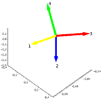
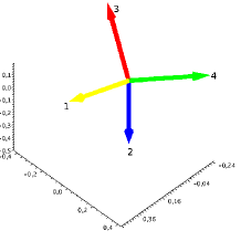
Figure 1: Tetrahedron configurations of the Pauli vectors

Labeling the vertices by the corresponding space-time points distinguishes an orientation of the tetrahedron; in particular, the two tetrahedra in Figure 1 cannot be mapped onto each other by an orientation-preserving rotation (22). This also implies that with the transformation (22) we cannot realize odd permutations of the space-time points. Hence the fermion system cannot be permutation symmetric, a contradiction.

Theorem 4.2 makes the effect of spontaneous symmetry breaking rigorous and shows that the fermionic projector induces non-trivial relations between the space-time points. But unfortunately, the theorem gives no information on what the resulting smaller outer symmetry group is, nor how the induced relations on the space-time points look like. For answering these questions, the setting of Theorem 4.2 is too general, because the particular form of our variational principle becomes important. The basic question is which symmetries the minimizers have. In [2] the minimizers of the critical action are constructed numerically for two particles and up to nine space-time points. For four space-time points, the Pauli vectors of the minimizers indeed form a tetrahedron. In Figure 2, the Pauli vectors of minimizers are shown in a few examples.

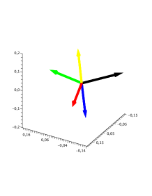
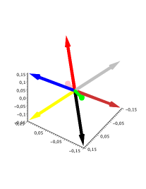
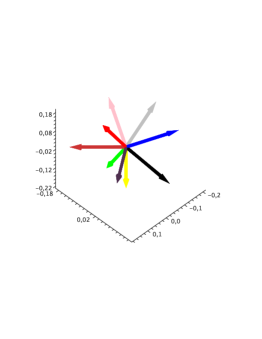
Figure 2: Pauli vectors of the minimizers for five, eight and nine space-time points

Qualitatively, one sees that for many space-time points, the vectors $\vec{v}_{x}$ all have approximately the same length $2/m$ and can thus be identified with points on a two-dimensional sphere of radius $2/m$. The critical variational principle aims at distributing these points uniformly on the sphere. The resulting structure is similar to a lattice on the sphere. Thus we can say that for the critical action in the case $f=2$ and in the limit $m\rightarrow\infty$, there is numerical evidence that the spontaneous symmetry breaking leads to the emergence of the structure of a two-dimensional lattice.

The above two-particle systems exemplify the spontaneous generation of additional structures in discrete space-time. However, one should keep in mind that for the transition to Minkowski space one needs to consider systems which involve many particles and are thus much more complicated. Before explaining how this transition is supposed to work, we need to consider how causality arises in the discrete framework.

5 Emergence of a Discrete Causal Structure

In an indefinite inner product space, the eigenvalues of a self-adjoint operator $A$ need not be real, but alternatively they can form complex conjugate pairs (see [10] or [5, Section 3]). This simple fact can be used to introduce a notion of causality.

Definition 5.1.

(discrete causal structure) Two discrete space-time points $x,y\in M$ are called timelike separated if the roots $\lambda_{j}$ of the characteristic polynomial of $A_{xy}$ are all real. They are said to be spacelike separated if all the $\lambda_{j}$ form complex conjugate pairs and all have the same absolute value.

As we shall see in Section 6 below, for Dirac spinors in Minkowski space this definition is consistent with the usual notion of causality. Moreover, the definition can be understood within discrete space-time in that it reflects the structure of the critical action. Namely, suppose that two space-time points $x$ and $y$ are spacelike separated. Then the critical Lagrangian (11) vanishes. A short calculation shows that the first variation ${\mathcal{M}}[A_{xy}]$, (12), also vanishes, and thus $A_{xy}$ does not enter the Euler-Lagrange equations. This can be seen in analogy to the usual notion of causality that points with spacelike separation cannot influence each other.

In [2, Section 5.2] an explicit example is given where the spontaneous symmetry breaking gives rise to a non-trivial discrete causal structure. We now outline this example, omitting a few technical details. We consider minimizers of the variational principle with constraint (7, 8) in the case $n=1$, $f=2$ and $m=3$. We found numerically that in the range of $\kappa$ under consideration here, the minimizers are permutation symmetric. Thus in view of (23, 24), the local correlation matrices are of the form (21) with

$$|\vec{v}_{x}|\;=:\;v\;\geq\;\frac{2}{3}\;=\;\rho_{x}\>,$$

and the three Pauli vectors form an equilateral triangle. In [2, Lemma 4.4] it is shown that any such choice of local correlation matrices can indeed be realized by a fermionic projector. Furthermore, it is shown that all fermionic projectors corresponding to the same value of $v$ are gauge equivalent. Thus we have, up to gauge transformations, a one-parameter family of fermionic projectors, parametrized by $v\geq 2/3$.

We again represent the fermionic projector as in (19). Then the closed chain can be written as

$$A_{xy}\;=\;\sum_{i,j=1}^{2}E_{x}\,u_{i}\mbox{\nolinebreak$>$}\mbox{$<\!\!$ \nolinebreak}u_{i}|E_{y}\,u_{j}\mbox{\nolinebreak$>$}\mbox{$<\!\!$ \nolinebreak}u_{j}|E_{x}\>.$$

Using the identity $\det(BC-\lambda)=\det(CB-\lambda)$, cyclically commuting the factors does not change the spectrum, and thus $A_{xy}$ is isospectral to the matrix

$$\sum_{i=1}^{2}\mbox{$<\!\!$ \nolinebreak}u_{j}|E_{x}\,u_{i}\mbox{\nolinebreak$>$}\mbox{$<\!\!$ \nolinebreak}u_{i}|E_{y}\,u_{k}\mbox{\nolinebreak$>$}\;=\;(F_{x}F_{y})_{jk}\>.$$

This makes it possible to express the roots $\lambda_{\pm}$ of the characteristic polynomial of $A_{xy}$ in terms of the local correlation matrices. A direct computation gives (see [2, Proposition 4.1])

$$\lambda_{\pm}\;=\;\frac{1}{4}\,\left(\rho_{x}\rho_{y}+\vec{v}_{x}\vec{v}_{y}\>\pm\>\sqrt{|\rho_{x}\vec{v}_{y}+\rho_{y}\vec{v}_{x}|^{2}-|\vec{v}_{x}\times\vec{v}_{y}|^{2}}\right)\>.$$

If $x=y$, the cross product vanishes, and thus the $\lambda_{\pm}$ are real. Hence each space-time point has timelike separation from itself (we remark that this is valid in general, see [2, Proposition 2.7] and [5, Lemma 4.2]). In the case $x\neq y$, the eigenvalues $\lambda_{+}$ and $\lambda_{-}$ are shown in Figure 3 for different values of $v$.

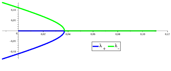
Figure 3: Plots of $\lambda_{+}$ and $\lambda_{-}$ in the complex plane for varying $v$.

If $v=2/3$, the eigenvalue $\lambda_{-}$ vanishes, whereas $\lambda_{+}=1/9$. If $v=\frac{4\sqrt{3}}{9}$, the values of $\lambda_{-}$ and $\lambda_{+}$ coincide. If $v$ is further increased, the $\lambda_{\pm}$ become complex and form a complex conjugate pair. Hence different space-time points have timelike separation if $v\leq\frac{4\sqrt{3}}{9}$, whereas they have spacelike separation if $v>\frac{4\sqrt{3}}{9}$. In the latter case the discrete causal structure is non-trivial, because some pairs of points have spacelike and other pairs timelike separation. Finally, a direct computation of the constraint (8) gives a relation between $v$ and $\kappa$. One finds that $v>\frac{4\sqrt{3}}{9}$ if and only if $\kappa>\frac{68}{81}$. We conclude that in the case $\kappa>\frac{68}{81}$, the spontaneous symmetry breaking leads to the emergence of non-trivial discrete causal structure.

We point out that the discrete causal structure of Definition 5.1 differs from the definition of a causal set (see [1]) in that it does not distinguish between future and past directed separations. In the above example with three space-time points, the resulting discrete causal structure is also a causal set, albeit in a rather trivial way where each point has timelike separation only from itself.

6 A First Connection to Minkowski Space

In this section we describe how to get a simple connection between discrete space-time and Minkowski space. In the last Sections 7–9 we will proceed by explaining the first steps towards making this intuitive picture precise. The simplest method for getting a correspondence to relativistic quantum mechanics in Minkowski space is to replace the discrete space-time points $M$ by the space-time continuum $\mathbb{R}^{4}$ and the sums over $M$ by space-time integrals. For a vector $\Psi\in H$, the corresponding localization $E_{x}\Psi$ should be a 4-component Dirac wave function, and the scalar product $\mbox{$<\!\!$ \nolinebreak}\Psi(x)\,|\,\Phi(x)\mbox{\nolinebreak$>$}$ on $E_{x}(H)$ should correspond to the usual Lorentz invariant scalar product on Dirac spinors $\overline{\Psi}\Phi$ with $\overline{\Psi}=\Psi^{\dagger}\gamma^{0}$ the adjoint spinor. Since this last scalar product is indefinite of signature $(2,2)$, we are led to choosing $n=2$. In view of (5), the discrete kernel should go over to the integral kernel of an operator $P$ on the Dirac wave functions,

$$(P\Psi)(x)\;=\;\int_{M}P(x,y)\,\Psi(y)\>d^{4}y\>.$$

The image of $P$ should be spanned by the occupied fermionic states. We take Dirac’s concept literally that in the vacuum all negative-energy states are occupied by fermions forming the so-called Dirac sea. Thus we are led to describe the vacuum by the integral over the lower mass shell

$$P(x,y)\;=\;\int\frac{d^{4}k}{(2\pi)^{4}}\>(k\mbox{ $/$}+m)\>\delta(k^{2}-m^{2})\>\Theta(-k^{0})\>e^{-ik(x-y)}$$

(here $\Theta$ is the Heaviside function). Likewise, if we consider several generations of particles, we take a sum of such Fourier integrals,

$$P(x,y)\;=\;\sum_{\beta=1}^{g}\rho_{\beta}\int\frac{d^{4}k}{(2\pi)^{4}}\>(k\mbox{ $/$}+m_{\beta})\>\delta(k^{2}-m_{\beta}^{2})\>\Theta(-k^{0})\>e^{-ik(x-y)}\>,$$ (25)

where $g$ denotes the number of generations, and the $\rho_{\beta}>0$ are weight factors for the individual Dirac seas (for a discussion of the weight factors see [7, Appendix A]). Computing the Fourier integrals, one sees that $P(x,y)$ is a smooth function, except on the light cone $\{(y-x)^{2}=0\}$, where it has poles and singular contributions (for more details see (41) below).

Let us find the connection between Definition 5.1 and the usual notion of causality in Minkowski space. Even without computing the Fourier integral (25), it is clear from the Lorentz symmetry that for every $x$ and $y$ for which the Fourier integral exists, $P(x,y)$ can be written as

$$P(x,y)\;=\;\alpha\,(y-x)_{j}\gamma^{j}+\beta\>\mbox{\rm 1 1}$$ (26)

with two complex coefficients $\alpha$ and $\beta$. Taking the complex conjugate of (25), we see that

$$P(y,x)\;=\;\overline{\alpha}\,(y-x)_{j}\gamma^{j}+\overline{\beta}\>\mbox{\rm 1 1}\>.$$

As a consequence,

$$A_{xy}\;=\;P(x,y)\,P(y,x)\;=\;a\,(y-x)_{j}\gamma^{j}+b\,\mbox{\rm 1 1}$$ (27)

with real parameters $a$ and $b$ given by

$$a\;=\;\alpha\overline{\beta}+\beta\overline{\alpha}\>,\;\;\;\;\;\;\;\;\;\;b\;=\;|\alpha|^{2}\,(y-x)^{2}+|\beta|^{2}\>,$$ (28)

where $(y-x)^{2}=(y-x)_{j}(y-x)^{j}$, and for the signature of the Minkowski metric we use the convention $(+--\,-)$. Applying the formula $(A_{xy}-b\mbox{\rm 1 1})^{2}=a^{2}\>(y-x)^{2}$, one can easily compute the roots of the characteristic polynomial of $A_{xy}$,

$$\lambda_{1}\;=\;\lambda_{2}\;=\;b+\sqrt{a^{2}\>(y-x)^{2}}\>,\;\;\;\;\;\;\;\;\;\;\lambda_{3}\;=\;\lambda_{4}\;=\;b-\sqrt{a^{2}\>(y-x)^{2}}\>.$$ (29)

If the vector $(y-x)$ is timelike, we see from the inequality $(y-x)^{2}>0$ that the $\lambda_{j}$ are all real. Conversely, if the vector $(y-x)$ is spacelike, the term $(y-x)^{2}<0$ is negative. As a consequence, the $\lambda_{j}$ form complex conjugate pairs and all have the same absolute value. This shows that for Dirac spinors in Minkowski space, Definition 5.1 is consistent with the usual notion of causality.

We next consider the Euler-Lagrange equations corresponding to the critical Lagrangian (11). If $(y-x)$ is spacelike, the $\lambda_{j}$ all have the same absolute value, and thus the Lagrangian vanishes. If on the other hand $(y-x)$ is timelike, the $\lambda_{j}$ as given by (29) are all real, and a simple computation using (28) yields that $\lambda_{1}\lambda_{2}\geq 0$, so that all the $\lambda_{j}$ have the same sign (we remark that this is true in more generality, see [7, Lemma 2.1]). Hence the Lagrangian (11) simplifies to

$${\mathcal{L}}[A_{xy}]\;=\;\left\{\begin{array}[]{cl}\displaystyle\mbox{\rm{Tr}\/}(A_{xy}^{2})-\frac{1}{4}\>\mbox{\rm{Tr}\/}(A_{xy})^{2}&{\mbox{if~{}$(y-x)$ is timelike}}\\[8.00003pt] 0&{\mbox{if~{}$(y-x)$ is spacelike}}\>.\end{array}\right.$$ (30)

Now we can compute the gradient (12) to obtain (for details see [7, Section 2.2])

$${\mathcal{M}}[A_{xy}]\;=\;\left\{\begin{array}[]{cl}\displaystyle 2A_{xy}-\frac{1}{2}\,\mbox{\rm{Tr}\/}(A_{xy})\,\mbox{\rm 1 1}&{\mbox{if~{}$(y-x)$ is timelike}}\\[8.00003pt] 0&{\mbox{if~{}$(y-x)$ is spacelike}}\>.\end{array}\right.$$ (31)

Using (27), we can also write this for timelike $(y-x)$ as

$${\mathcal{M}}[A_{xy}]\;=\;2a(x,y)\>(y-x)^{j}\gamma_{j}\>.$$ (32)

Furthermore, using (28) we obtain that

$${\mathcal{M}}[A_{xy}]\;=\;{\mathcal{M}}[A_{yx}]\>.$$ (33)

Combining the relations (33, 32, 26), we find that the two summands in (13) coincide, and thus

$$Q(x,y)\;=\;\frac{1}{2}\>{\mathcal{M}}[A_{xy}]\>P(x,y)$$ (34)

(we remark that the last identity holds in full generality, see [4, Lemma 5.2.1]).

We point out that this calculation does not determine ${\mathcal{M}}$ on the light cone, and due to the singularities of $P(x,y)$, the Lagrangian is indeed ill-defined if $(y-x)^{2}=0$. However, as an important special feature of the critical Lagrangian, we can make sense of the Euler-Lagrange equations (15), if we only assume that ${\mathcal{M}}$ is well-defined as a distribution. We now explain this argument, which will be crucial for the considerations in Sections 8 and 9. More precisely, we assume that the gradient of the critical Lagrangian is a Lorentz invariant distribution, which away from the light cone coincides with (31), has a vector structure (32) and is symmetric (33). Then this distribution, which we denote for clarity by $\tilde{\mathcal{M}}$, can be written as

$$\tilde{\mathcal{M}}(\xi)\;=\;2\,\xi\mbox{ $/$}\>a(\xi^{2})\>\Theta(\xi^{2})\,\epsilon(\xi^{0})\>,$$ (35)

where we set $\xi\equiv y-x$ and $\xi\mbox{ $/$}\equiv\xi^{j}\gamma_{j}$, and $\epsilon$ is the step function (defined by $\epsilon(x)=1$ if $x\geq 0$ and $\epsilon(x)=-1$ otherwise). We now consider the Fourier transform of the distribution $\tilde{\mathcal{M}}(\xi)$, denoted by $\hat{\mathcal{M}}(k)$. The factor $\xi\mbox{ $/$}$ corresponds to the differential operator $i\mbox{$\partial$ $/$}_{k}$ in momentum space, and thus

$$\hat{\mathcal{M}}(k)\;=\;2i\,\mbox{$\partial$ $/$}_{k}\int d^{4}\xi\>a(\xi^{2})\>\Theta(\xi^{2})\,\epsilon(\xi^{0})\>e^{-ik\xi}\>.$$ (36)

This Fourier integral vanishes if $k^{2}<0$. Namely, due to Lorentz symmetry, in this case we may assume that $k$ is purely spatial, $k=(0,\vec{k})$. But then the integrand of the time integral in (36) is odd because of the step function, and thus the whole integral vanishes. As in [4], we denote the mass cone as well as the upper and lower mass cone by

$${\mathcal{C}}=\{k\>|\>k^{2}>0\}\>,\quad{\mathcal{C}}^{\vee}=\{k\in{\mathcal{C}}\>|\>k^{0}>0\}\>,\quad{\mathcal{C}}^{\wedge}=\{k\in{\mathcal{C}}\>|\>k^{0}<0\}\>,$$ (37)

respectively. Then the above argument shows that the distribution $\hat{\mathcal{M}}$ is supported in the closed mass cone, ${\mbox{supp}}\,\hat{\mathcal{M}}\subset\overline{\mathcal{C}}$. Next we rewrite the pointwise product in (34) as a convolution in momentum space,

$$\hat{Q}(q)\;=\;\frac{1}{2}\>(\hat{\mathcal{M}}*\hat{P})(q)\;=\;\frac{1}{2}\int\frac{d^{4}p}{(2\pi)^{4}}\>\hat{\mathcal{M}}(p)\>\hat{P}(q-p)\>.$$ (38)

If $q$ is in the lower mass cone ${\mathcal{C}}^{\wedge}$, the integrand of the convolution has compact support (see Figure 4), and the integral is finite

Figure 4: The convolution ${\hat{\mathcal{M}}}*\hat{P}$.

(if however $q\not\in\overline{\mathcal{C}^{\wedge}}$, the convolution integral extends over an unbounded region and is indeed ill-defined). We conclude that $\hat{Q}(q)$ is well-defined inside the lower mass cone. Since the fermionic projector (25) is also supported in the lower mass cone, this is precisely what we need in order to make sense of the operator products $\hat{P}(k)\,\hat{\mathcal{M}}(k)$ and $\tilde{\mathcal{M}}(k)\,\hat{P}(k)$ which appear in the commutator (15). In this way we have given the Euler-Lagrange equations a mathematical meaning.

In the above consideration we only considered the critical Lagrangian. To avoid misunderstandings, we now briefly mention the physical significance of the variational principle with constraint (7, 8) and explain the connection to the above arguments. In order to describe a realistic physical system involving different types of fermions including left-handed neutrinos, for the fermionic projector of the vacuum one takes a direct sum of fermionic projectors of the form (25) (for details see [4, §5.1]). On the direct summands involving the neutrinos, the closed chain $A_{xy}$ vanishes identically, and also the Euler-Lagrange equations are trivially satisfied. On all the other direct summands, we want the operator ${\mathcal{M}}$ to be of the form (35), so that the above considerations apply again. In order to arrange this, the value of the Lagrange multiplier $\mu$ must be larger than the critical value $\frac{1}{2n}$. Thus we are in the case $\mu>\frac{1}{2n}$ where the auxiliary variational principle has no minimizers. This is why we need to consider the variational principle with constraint (7, 8). Hence the fermionic projector of fundamental physics should be a minimizer of the variational principle with constraint (7, 8) corresponding to a value $\mu>\frac{1}{2n}$ of the Lagrange multiplier (such minimizers with $\mu>\frac{1}{2n}$ indeed exist, see [2, Proposition 5.2] for a simple example). The physical significance of the critical variational principle lies in the fact that restricting attention to one direct summand of the form (25) (or more generally to a subsystem which does not involve chiral particles), the Euler-Lagrange equations corresponding to (7, 8) coincide with those for the critical Lagrangian as discussed above. For more details we refer to [4, Chapter 5].

7 A Static and Isotropic Lattice Model

Our concept is that for many particles and many space-time points, the mechanism explained in Sections 4 and 5 should lead to the spontaneous emergence of the structure of Minkowski space or a Lorentzian manifold. The transition between discrete space-time and the space-time continuum could be made precise by proving conjectures of the following type.

Conjecture 7.1.

In spin dimension $(2,2)$, there is a series of fermion systems in discrete space-time $(H^{(l)},\mbox{$<\!\!$ \nolinebreak}.|.\mbox{\nolinebreak$>$},(E_{x}^{(l)})_{x\in M^{(l)}},P^{(l)})$ with the following properties:

• The fermionic projectors $P^{(l)}$ are minimizers of the auxiliary variational principle (9) in the critical case $\mu=\frac{1}{4}$.

• The number of space-time points $m^{(l)}$ and the number of particles $f^{(l)}$ scale in $l$ as follows,

  $$m^{(l)}\;\sim\;l^{4}\>,\qquad f^{(l)}\;\sim\;l^{3}\>.$$

• There are positive constants $c^{(l)}$, embeddings $\iota^{(l)}\>:\>M^{(l)}\hookrightarrow\mathbb{R}^{4}$ and isomorphisms $\alpha^{(l)}\>:\>H^{(l)}\rightarrow L^{2}(\Phi^{(l)}(M^{(l)}),\mbox{$<\!\!$ \nolinebreak}.|.\mbox{\nolinebreak$>$})$ (where $\mbox{$<\!\!$ \nolinebreak}.|.\mbox{\nolinebreak$>$}$ is the standard inner product on Dirac spinors $\mbox{$<\!\!$ \nolinebreak}\Phi|\Psi\mbox{\nolinebreak$>$}=\Phi^{\dagger}\gamma^{0}\Psi$), such that for any test wave functions $\Psi,\Phi\in C^{\infty}_{0}(\mathbb{R}^{4})^{4}$,

  $$c^{(l)}\!\!\!\!\!\sum_{x,y\in M^{(l)}}\!\!\!\Phi(\iota x)^{\dagger}\alpha^{(l)}E^{(l)}_{x}P^{(l)}E_{y}^{(l)}(\alpha^{(l)})^{-1}\Psi(\iota y)$$

  $$\;\;\;\;\;\;\;\;\;\;\stackrel{{\scriptstyle l\rightarrow\infty}}{{\longrightarrow}}\int d^{4}x\int d^{4}y\>\Phi(x)^{\dagger}P(x,y)\,\Psi(y)\>,$$

  where $P(x,y)$ is the distribution (25).

• As $l\rightarrow\infty$, the operators ${\mathcal{M}}[A^{(l)}_{xy}]$ converge likewise to the distribution $\tilde{\mathcal{M}}(\xi)$, (35).

Similarly, one can formulate corresponding conjectures for systems involving several Dirac seas, where the variational principle (7) with constraint (8) should be used if chiral particles are involved. Moreover, it would be desirable to specify that minimizers of the above form are in some sense generic. Ultimately, one would like to prove that under suitable generic conditions, every sequence of minimizing fermion systems has a subsequence which converges in the above weak sense to an interacting physical system defined on a Lorentzian manifold.

Proving such conjectures is certainly difficult. In preparation, it seems a good idea to analyze particular aspects of the problem. One important task is to understand why discrete versions of Dirac sea configurations (25) minimize the critical action. A possible approach is to analyze discrete fermion systems numerically. In order to compare the results in a reasonable way to the continuum, one clearly needs systems involving many space-time points and many particles. Unfortunately, large discrete systems are difficult to analyze numerically. Therefore, it seems a good idea to begin the numerical analysis with simplified systems, which capture essential properties of the original system but are easier to handle. In [9] such a simplified system is proposed, where we employ a spherically symmetric and static ansatz for the fermionic projector. We now briefly outline the derivation of this model and discuss a few results.

For the derivation we begin in Minkowski space with a static and isotropic system, which means that the fermionic projector $P(x,y)$ depends only on the difference $\xi=y-x$ and is spherically symmetric. We take the Fourier transform,

$$P(\xi)\;=\;\int\frac{d^{4}p}{(2\pi)^{4}}\>\hat{P}(p)\>e^{ip\xi}\>,$$ (39)

and take for $\hat{P}$ an ansatz involving a vector-scalar structure, i.e.

$$\hat{P}(p)\;=\;v_{j}(p)\,\gamma^{j}+\phi(p)\,\mbox{\rm 1 1}$$ (40)

with real functions $v_{j}$ and $\phi$. Using the spherical symmetry, we can choose polar coordinates and carry out the angular integrals in (39). This leaves us with a two-dimensional Fourier integral from the momentum variables $(\omega=p^{0},k=|\vec{p}|)$ to the position variables $(t=\xi^{0},r=|\vec{\xi}|)$. In order to discretize the system, we restrict the position variables to a finite lattice ${\mathfrak{L}}$,

$$(t,r)\;\in\;{\mathfrak{L}}\;:=\;\Big{\{}0,2\pi,\ldots,\,2\pi(N_{t}-1)\Big{\}}\times\Big{\{}0,2\pi,\ldots,\,2\pi(N_{r}-1)\Big{\}}\>.$$

Here the integer parameters $N_{t}$ and $N_{r}$ describe the size of the lattice, and by scaling we arranged that the lattice spacing is equal to $2\pi$. Then the momentum variables are on the corresponding dual lattice $\hat{{\mathfrak{L}}}$,

$$(\omega,k)\;\in\;\hat{{\mathfrak{L}}}\;:=\;\Big{\{}-(N_{t}-1),\ldots,-1,0\Big{\}}\times\Big{\{}1,\ldots,N_{r}\Big{\}}\>.$$

Defining the closed chain by $A(t,r)=P(t,r)P(t,r)^{*}$, we can again introduce the critical Lagrangian (10) with $\mu=\frac{1}{4}$. For the action, we modify (9) to

$${\mathcal{S}}[P]\;=\;\sum_{(t,r)\in{\mathfrak{L}}}\rho_{t}(t)\,\rho_{r}(r)\>{\mathcal{L}}(t,r)\>,$$

where the weight factors $\rho_{t}$ and $\rho_{r}$ take into account that we only consider positive $t$ and that a point $(t,r)$ corresponds to many states on a sphere of radius $r$. When varying the action we need to take into account two constraints, called the trace condition and the normalization condition, which take into account that the total number of particles is fixed and that the fermionic projector should be idempotent.

In [9, Proposition 6.1] the existence of minimizers is proved, and we also present first numerical results for a small lattice system. More precisely, we consider an $8\times 6$-lattice and occupy one state with $k=1$ and one with $k=2$. The absolute minimum is attained when occupying the lattice points $(\omega_{1}=-1,k=1)$ and $(\omega_{2}=-2,k=2)$. Introducing a parameter $\tau$ by the requirement that the spatial component of the vector $v$ in (40) should satisfy the relation $|\vec{v}|=\phi\,\sinh\tau$, the trace and normalization conditions fix our system up to the free parameters $\tau_{1}$ and $\tau_{2}$ at the two occupied space-time points. In Figure 5 the action is shown as a function of these two free parameters.

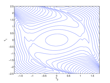
Figure 5: Action for a lattice system with two occupied states

The minimum at the origin corresponds to the trivial configuration where the two vectors $v_{i}$ are both parallel to the $\omega$-axis. However, this is only a local minimum, whereas the absolute minimum of the action is attained at the two non-trivial points $(\tau_{1}\approx 1.5,\tau_{2}\approx 1)$ and $(\tau_{1}\approx-1.5,\tau_{2}\approx-1)$.

Obviously, a sytem of two occupied states on an $8\times 6$-lattice is much too small for modelling a Dirac sea structure. But at least, our example shows that our variational principle generates a non-trivial structure on the lattice where the occupied points distinguish specific lattice points, and the corresponding vectors $v$ are not all parallel.

8 Analysis of Regularization Tails

Another important task in making the connection to Minkowski space rigorous is to justify the distribution $\tilde{\mathcal{M}}$ in (35). To explain the difficulty, let us assume that we have a family of fermion systems $(H^{(l)},\mbox{$<\!\!$ \nolinebreak}.|.\mbox{\nolinebreak$>$},(E_{x}^{(l)})_{x\in M^{(l)}},P^{(l)})$ having the properties (1)-(3) of Conjecture 7.1. We can then regard the operators $\alpha^{(l)}P^{(l)}(\alpha^{(l)})^{-1}$ as regularizations of the continuum fermionic projector (25). It is easier to consider more generally a family of regularizations $(P^{\varepsilon})_{\varepsilon>0}$ in Minkowski space with

$$P^{\varepsilon}(x,y)\;\stackrel{{\scriptstyle\varepsilon\searrow 0}}{{\longrightarrow}}\;P(x,y)\quad{\mbox{in the distributional sense}}.$$

The parameter $\varepsilon$ should be the length scale of the regularization. In order to justify (35) as well as the convolution integral (38), our regularization should have the following properties:

Definition 8.1.

The fermionic projector satisfies the assumption of a distributional ${\mathcal{M}}P$-product if the following conditions are satisfied:

• There is a distribution $\tilde{\mathcal{M}}(\xi)$ of the form (35) such that $\lim_{\varepsilon\searrow 0}{\mathcal{M}}[A^{\varepsilon}_{xy}]=\tilde{\mathcal{M}}(\xi)$ in the distributional sense.

• For every $k$ for which $\lim_{\varepsilon\searrow 0}\hat{Q}^{\varepsilon}(k)$ exists, the convolution integral (38) is well-defined and $\lim_{\varepsilon\searrow 0}\hat{Q}^{\varepsilon}(k)=\hat{Q}(k)$.

This notion was introduced in [4, §5.6] and used as an ad-hoc assumption on the regularization. Justifying this assumption is not just a technicality, but seems essential for getting a detailed understanding of how the connection between discrete space-time and Minkowski space is supposed to work. Namely, if one takes a simple ultraviolet regularization (for example a cutoff in momentum space), then, due to the distributional singularity of $P(x,y)$ on the light cone, the product $A^{\varepsilon}_{xy}=P^{\varepsilon}(x,y)P^{\varepsilon}(y,x)$ will in the limit $\varepsilon\searrow 0$ develop singularities on the light cone, which are ill-defined even in the distributional sense. Thus, in order to satisfy the conditions of Definition 8.1, we need to construct special regularizations, such that the divergences on the light cone cancel. In [7] it is shown that this can indeed be accomplished. The method is to consider a class of spherically symmetric regularizations involving many free parameters, and to adjust these parameters such that all the divergences on the light cone and near the origin compensate each other. It seems miraculous that it is possible to cancel all the divergences; this can be regarded as a confirmation for our approach. If one believes that the regularized fermionic projector describes nature, we get concrete hints on how the vacuum should look like on the Planck scale. More specifically, the admissible regularizations give rise to a multi-layer structure near the light cone involving several length scales.

In this survey article we cannot enter into the constructions of [7]. Instead, we describe a particular property of Dirac sea configurations which is crucial for making the constructions work. Near the light cone, the distribution $P(x,y)$ has an expansion of the following form

$$P(x,y) = +iC_{0}\>\xi\mbox{ $/$}\>\frac{\mbox{PP}}{\xi^{4}}+C_{1}\>\frac{\mbox{PP}}{\xi^{2}}+iC_{2}\>\xi\mbox{ $/$}\>\frac{\mbox{PP}}{\xi^{2}}+C_{3}\,\log(\xi^{2})+\cdots$$ (41)

$$+\epsilon(\xi^{0})\Big{(}D_{0}\>\xi\mbox{ $/$}\delta^{\prime}(\xi^{2})+iD_{1}\>\delta(\xi^{2})+D_{2}\>\xi\mbox{ $/$}\delta(\xi^{2})+iD_{3}\>\Theta(\xi^{2})+\cdots\Big{)}\qquad$$

with real constants $C_{j}$ and $D_{j}$ (PP denotes the principal part; for more details see [7, Section 3]). Let us consider the expression ${\mathcal{M}}[A_{xy}]$, (31), for timelike $\xi$. Computing the closed chain by $A_{xy}=P(x,y)\,P(x,y)^{*}$, from (41) we obtain away from the light cone the expansion

$$A_{xy}\;=\;\frac{C_{0}^{2}}{\xi^{6}}+\frac{C_{1}^{2}+2C_{0}C_{2}}{\xi^{4}}+2C_{0}D_{3}\>\frac{\xi\mbox{ $/$}\>\epsilon(\xi^{0})}{\xi^{4}}\>+\>\cdots\qquad(\xi^{2}>0).$$ (42)

It is remarkable that there is no contribution proportional to $\xi\mbox{ $/$}/\xi^{6}$. This is because the term $\sim C_{0}C_{1}$ is imaginary, and because the contributions corresponding to $D_{0}$, $D_{1}$ and $D_{2}$ are supported on the light cone. Taking the trace-free part, we find

$${\mathcal{M}}[A_{xy}]\;=\;4C_{0}D_{3}\>\frac{\xi\mbox{ $/$}\,\epsilon(\xi^{0})}{\xi^{4}}\>+\>\cdots\qquad(\xi^{2}>0).$$ (43)

The important point is that, due to the specific form of the Dirac sea configuration, the leading pole of ${\mathcal{M}}[A_{xy}]$ on the light cone is of lower order than expected from a naive scaling. This fact is extremely useful in the constructions of [7]. Namely, if we consider regularizations of the distribution (41), the terms corresponding to $C_{0}$, $C_{1}$ and $C_{2}$ will be “smeared out” and will thus no longer be supported on the light cone. In particular, the contribution $\sim C_{0}D_{1}$ no longer vanishes, and this vector contribution can be used to modify (43). In simple terms, this effect means that the contributions by the regularization are amplified, making it possible to modify ${\mathcal{M}}[A^{\varepsilon}_{xy}]$ drastically by small regularization terms. In [7] we work with regularization tails, which are very small but spread out on a large scale $\varepsilon^{\gamma}$ with $\gamma<1$. Taking many tails with different scales gives rise to the above-mentioned multi-layer structure. Another important effect is that the the regularization yields bilinear contributions to ${\mathcal{M}}[A^{\varepsilon}_{xy}]$ of the form $\sim iC_{0}D_{0}\gamma^{t}\gamma^{r}$ (with $\gamma^{r}=\vec{\xi}\vec{\gamma}/|\vec{\xi}|$), which are even more singular on the light cone than the vector contributions. The bilinear contributions tend to make the roots $\lambda_{j}$ complex (as can be understood already from the fact that $(i\gamma^{t}\gamma^{r})^{2}=-\mbox{\rm 1 1}$). This can be used to make a neighborhood of the light cone space-like; more precisely,

$${\mathcal{M}}[A^{\varepsilon}_{xy}]\;\equiv\;0\qquad{\mbox{if~{}$|\xi^{0}|<|\vec{\xi}|+\epsilon^{\gamma}\,|\vec{\xi}|^{-\frac{1}{\alpha}}$ with~{}$\gamma<1$ and~{}$\alpha>1$}}.$$ (44)

The analysis in [7] also specifies the singularities of the distribution $\tilde{\mathcal{M}}$ on the light cone (recall that by (31), $\tilde{\mathcal{M}}$ is determined only away from the light cone). We find that $\tilde{\mathcal{M}}$ is unique up to the contributions

$$\tilde{\mathcal{M}}(x,y)\;\asymp\;c_{0}\>\xi\mbox{ $/$}\>\delta^{\prime}(\xi^{2})\>\epsilon(\xi^{0})\>+\>c_{1}\>\xi\mbox{ $/$}\>\delta(\xi^{2})\>\epsilon(\xi^{0})$$ (45)

with two free parameters $c_{0},c_{1}\in\mathbb{R}$. Moreover, the regularization tails give us additional freedom to modify ${\mathcal{M}}[A^{\varepsilon}_{xy}]$ near the origin $\xi=0$. This makes it possible to go beyond the distributional ${\mathcal{M}}P$-product by arranging extra contributions supported at the origin. Expressed in momentum space, we may modify $\hat{Q}(q)$ by a polynomial in $Q$; namely (see [7, Theorem 2.4])

$$\hat{Q}(q)\;:=\;\lim_{\varepsilon\searrow 0}\hat{Q}^{\varepsilon}(q)\;=\ \frac{1}{2}\>(\hat{\mathcal{M}}*\hat{P})(q)+c_{2}+c_{3}\,q\!\!\!/+c_{4}\,q^{2}\qquad(q\in{\mathcal{C}}^{\wedge})$$ (46)

with additional free parameters $c_{2},c_{3},c_{4}\in\mathbb{R}$.

9 A Variational Principle for the Masses of the Dirac Seas

With the analysis of the regularization tails in the previous section we have given the Euler-Lagrange equations for a vacuum Dirac sea configuration a rigorous mathematical meaning. All the formulas are well-defined in Minkowski space without any regularization. The freedom to choose the regularization of the fermionic projector is reflected by the free real parameters $c_{0},\ldots,c_{4}$ in (45) and (46). This result is the basis for a more detailed analysis of the Euler-Lagrange equations for vacuum Dirac sea configurations as carried out recently in [8]. We now outline the methods and results of this paper.

We first recall the notion of state stability as introduced in [4, §5.6]. We want to analyze whether the vacuum Dirac sea configuration is a stable local minimum of the critical variational principle within the class of static and homogeneous fermionic projectors in Minkowski space. Thus we consider variations where we take an occupied state of one of the Dirac seas and bring the corresponding particle to any other unoccupied state $q\in{\mathcal{Q}}^{\wedge}$. Taking into account the vector-scalar structure in the ansatz (25) and the negative definite signature of the fermionic states, we are led to the variations (for details see [4, §5.6])

$$\delta P=-c(k\mbox{ $/$}+m)\>e^{-ik(x-y)}+c(l\!\!/+m)\>e^{-iq(x-y)}$$ (47)

with $m\in\{m_{1},\ldots,m_{g}\}\not\ni\sqrt{q^{2}}$, $k^{2}=l^{2}=m^{2}$ and $k^{0},l^{0}<0$. We demand that such variations should not decrease the action,

$$S[P+\delta P]\;\geq\;S[P]\quad\mbox{for all variations~{}(\ref{varstat})}.$$

For the proper normalization of the fermionic states, we need to consider the system in finite $3$-volume. Since the normalization constant $c$ in (47) tends to zero in the infinite volume limit, we may treat $\delta S$ as a first order perturbation. Hence computing the variation of the action by (14), we obtain the condition stated in the next definition. Note that, according to (45), (46) and (38), we already know that $\hat{Q}$ is well-defined inside the lower mass cone and has a vector scalar structure, i.e.

$$\hat{Q}(k)\;=\;a\>\frac{k\mbox{ $/$}}{|k|}+b\>,\qquad k\in{\mathcal{C}}^{\wedge}\>,$$ (48)

where we set $|k|=\sqrt{k^{2}}$, and $a=a(k^{2})$, $b=b(k^{2})$ are two real-valued, Lorentz invariant functions.

Definition 9.1.

The fermionic projector of the vacuum is called state stable if the functions $a$ and $b$ in the representation (48) of $\hat{Q}(k)$ have the following properties:

• $a$ is non-negative.

• The function $a+b$ is minimal on the mass shells,

  $$(a+b)(m^{2}_{\alpha})\;=\;\inf_{q\in{\mathcal{C}}^{\land}}(a+b)(q^{2})\qquad\mbox{for all~{}$\alpha\in\{1,\ldots,g\}$}.$$ (49)

It is very helpful for the understanding and the analysis of state stability that the condition (49) can be related to the Euler-Lagrange equations of a corresponding variational principle. This variational principle was introduced in [8] for unregularized Dirac sea configurations of the form (25) and can be regarded as a Lorentz invariant analog of the critical variational principle. To define this variational principle, we expand the trace-free part of the closed chain inside the light cone similar to (41, 42) as follows,

$$A_{0}(\xi)\;:=\;A_{xy}-\frac{1}{4}\>\mbox{\rm{Tr}\/}(A_{xy})\;=\;\xi\mbox{ $/$}\>\epsilon(\xi^{0})\left(\frac{{\mathfrak{m}}_{3}}{\xi^{4}}+\frac{{\mathfrak{m}}_{5}}{\xi^{2}}+{\mathcal{O}}(\log\xi^{2})\right),$$

where the coefficients ${\mathfrak{m}}_{3}$ and ${\mathfrak{m}}_{5}$ are functions of the parameters $\rho_{\beta}$ and $m_{\beta}$ in (25). Using the simplified form (30) of the critical Lagrangian, we thus obtain for $\xi$ in the interior of the light cone the expansion

$${\mathcal{L}}\;=\;\mbox{\rm{Tr}\/}(A_{0}(\xi)^{2})\;=\;\frac{{\mathfrak{m}}_{3}}{\xi^{6}}+\frac{2{\mathfrak{m}}_{3}{\mathfrak{m}}_{5}}{\xi^{4}}+{\mathcal{O}}(\xi^{-2}\log\xi^{2})\qquad(\xi^{2}>0).$$

The naive adaptation of the critical action (9) would be to integrate ${\mathcal{L}}$ over the set $\{\xi^{2}>0\}$ (for details see [8, Section 2]). However, this integral diverges because the hyperbolas $\{\xi^{2}={\mbox{const}}\}$, where ${\mathcal{L}}$ is constant, have infinite measure. To avoid this problem, we introduce the variable $z=\xi^{2}$ and consider instead the one-dimensional integral $\int_{0}^{\infty}{\mathcal{L}}(z)\,z\,dz$, which has the same dimension of length as the integral $\int{\mathcal{L}}\,d^{4}\xi$. Since this new integral is still divergent near $z=0$, we subtract suitable counter terms and set

$${\mathcal{S}}\;=\;\lim_{\varepsilon\searrow 0}\left(\int_{\varepsilon}^{\infty}{\mathcal{L}}(z)\>z\,dz\>-\>\frac{{\mathfrak{m}}_{3}^{2}}{\varepsilon}\>+\>2\,{\mathfrak{m}}_{3}\,{\mathfrak{m}}_{5}\,\log\varepsilon\right).$$ (50)

In order to build in the free parameters $c_{0},c_{1}$ in (45) and $c_{2},c_{3}$ in (46), we introduce the extended action by adding extra terms,

$${\mathcal{S}}_{\mbox{\scriptsize{ext}}}\;=\;{\mathcal{S}}\>+\>F({\mathfrak{m}}_{3},{\mathfrak{m}}_{5})+c_{3}\sum_{\beta=1}^{g}\rho_{\beta}\,m_{\beta}^{4}+c_{4}\sum_{\beta=1}^{g}\rho_{\beta}\,m_{\beta}^{5}\>,$$ (51)

where $F$ is an arbitrary real function (note that the parameter $c_{2}$ in (46) is irrelevant for state stability because it merely changes the function $b$ in (48) by a constant). In our Lorentz invariant variational principle we minimize (51), varying the parameters $\rho_{\beta}$ and $m_{\beta}$ under the constraint

$$\sum_{\beta=1}^{g}m_{\beta}\,\rho_{\beta}^{3}\;=\;{\mbox{const}}\>.$$

This constraint is needed to rule out trivial minimizers; it can be understood as replacing the condition in discrete space-time that the number of particles is fixed.

In [8] it is shown that, allowing for an additional “test Dirac sea” of mass $m_{g+1}$ and weight $\rho_{g+1}$ (with $\rho_{g+1}=0$ but $\delta\rho_{g+1}\neq 0$), the corresponding Euler-Lagrange equations coincide with (49). The difficult point in the derivation is to take the Fourier transform of the Lorentz invariant action and to reformulate the $\varepsilon$-regularization in (50) in momentum space. In [8] we proceed by constructing numerical solutions of the Euler-Lagrange equations which in addition satisfy the condition (1) in Definition 9.1. We thus obtain state stable Dirac sea configurations. Figure 6

Figure 6: A state stable Dirac sea structure with three generations

shows an example with three generations and corresponding values of the parameters $m_{1}=1$, $m_{2}=5$, $m_{3}=20$ and $\rho_{1}=1$, $\rho_{2}=10^{-4}$, $\rho_{3}=9.696\times 10^{-6}$.

10 The Continuum Limit

The continuum limit provides a method for analyzing the Euler-Lagrange equations (15) for interacting systems in Minkowski space. For details and results we refer to [4, Chapters 6-8]; here we merely put the procedure of the continuum limit in the context of the methods outlined in Sections 6–9. As explained in Section 8, the regularization yields bilinear contributions to $A^{\varepsilon}_{xy}$, which make a neighborhood of the light cone spacelike (44). Hence near the light cone, the roots $\lambda_{j}$ of the characteristic polynomial form complex conjugate pairs and all have the same absolute value,

$$|\lambda_{i}|=|\lambda_{j}|\qquad{\mbox{for all~{}$i,j$}},$$ (52)

so that the critical Lagrangian (11) vanishes identically. If we introduce an interaction (for example an additional Dirac wave function or a classical gauge field), the corresponding perturbation of the fermionic projector will violate (52). We thus obtain corresponding contributions to ${\mathcal{M}}[A^{\varepsilon}_{xy}]$ in a strip of size $\sim\varepsilon$ around the light cone. These contributions diverge if the regularization is removed. For small $\varepsilon$, they are much larger than the contributions by the regularization tails as discussed in Section 8; this can be understood from the fact that they are much closer to the light cone. The formalism of the continuum limit is obtained by an expansion of these divergent contributions in powers of the regularization length $\varepsilon$. The dependence of the expansion coefficients on the regularization is analyzed using the method of variable regularization; we find that this dependence can be described by a small number of free parameters, which take into account the unknown structure of space-time on the Planck scale. The dependence on the gauge fields can be analyzed explicitly using the method of integration along characteristics or, more systematically, by performing a light-cone expansion of the fermionic projector. In this way, one can relate the Euler-Lagrange equations to an effective interaction in the framework of second quantized Dirac fields and classical bosonic fields.

11 Outlook and Open Problems

In this paper we gave a detailed picture of the transition from discrete space-time to the usual space-time continuum. Certain aspects have already been worked out rigorously. But clearly many questions are still open. Generally speaking, the main task for making the connection between discrete space-time and Minkowski space rigorous is to clarify the symmetries and the discrete causal structure of the minimizers for discrete systems involving many particles and many space-time points. More specifically, we see the following directions for future work:

1. Numerics for large lattice models: The most direct method to clarify the connection between discrete and continuous models is to the static and isotropic lattice model [9] for systems which are so large that they can be compared in a reasonable way to the continuum. Important questions are whether the minimizers correspond to Dirac sea configurations and what the resulting discrete causal structure is. The next step will be to analyze the connection to the regularization effects described in [7]. In particular, does the lattice model give rise to a multi-layer structure near the light cone? What are the resulting values of the constants $c_{0},\ldots,c_{4}$ in (45, 46)?

2. Numerics for fermion systems in discrete space-time: For more than two particles, almost nothing is known about the minimizers of our variational principles. A systematic numerical study could answer the question whether for many particles and many space-time points, the minimizers have outer symmetries which can be associated to an underlying lattice structure. A numerical analysis of fermion systems in discrete space-time could also justify the spherically symmetric and static ansatz in [9].

3. Analysis and estimates for discrete systems: In the critical case, the general existence problem for minimizers is still open. Furthermore, using methods of [6], one can study fermion systems with prescribed outer symmetry analytically. One question of interest is whether for minimizers the discrete causal structure is compatible with the structure of a corresponding causal set. It would be extremely useful to have a method for analyzing the minimizers asymptotically for a large number of space-time points and many particles. As a first step, a good approximation technique (maybe using methods from quantum statistics?) would be very helpful.

4. Analysis of the Lorentz invariant variational principle: In [8] the variational principle for the masses of the vacuum Dirac seas is introduced and analyzed. However, the existence theory has not yet been developed. Furthermore, the structure of the minimizers still needs to be worked out systematically.

5. Analysis of the continuum limit: It is a major task to analyze the continuum limit in more detail. The next steps are the derivation of the field equations and the analysis of the spontaneous symmetry breaking of the chiral gauge group. Furthermore, except for [3, Appendix B], no calculations for gravitational fields have been made so far. The analysis of the continuum limit should also give constraints for the weight factors $\rho_{\beta}$ in (25) (see [8, Appendix A]).

6. Field quantization: As explained in [4, §3.6], the field quantization effects should be a consequence of a “discreteness” of the interaction described by our variational principle. This effect could be studied and made precise for small discrete systems.

Apart from being a challenge for mathematics, these problems have the physical perspective of clarifying the microscopic structure of our universe and explaining the emergence of space and time.

References

- [1] L. Bombelli, J. Lee, D. Meyer, R. Sorkin, “Space-time as a causal set,” Phys. Rev. Lett. 59 (1987) 521-524
- [2] A. Diethert, F. Finster, D. Schiefeneder, “Fermion systems in discrete space-time exemplifying the spontaneous generation of a causal structure,” arXiv:0710.4420 [math-ph] (2007)
- [3] F. Finster, “Light-cone expansion of the Dirac sea to first order in the external potential,” hep-th/9707128, Michigan Math. J. 46 (1999) 377-408
- [4] F. Finster, “The Principle of the Fermionic Projector,” AMS/IP Studies in Advanced Mathematics 35 (2006)
- [5] F. Finster, “A variational principle in discrete space-time – existence of minimizers,” math-ph/0503069, Calc. Var. and Partial Diff. Eq. 29 (2007) 431-453
- [6] F. Finster, “Fermion systems in discrete space-time – outer symmetries and spontaneous symmetry breaking,” math-ph/0601039, Adv. Theor. Math. Phys. 11 (2007) 91-146
- [7] F. Finster, “On the regularized fermionic projector of the vacuum,” math-ph/0612003v2, to appear in J. Math. Phys. (2008)
- [8] F. Finster, S. Hoch, “An action principle for the masses of Dirac particles,” arXiv:0712.0678 [math-ph] (2007)
- [9] F. Finster, W. Plaum, “A lattice model for the fermionic projector in a static and isotropic space-time,” arXiv:0712.0676 [math-ph], to appear in Math. Nachr. (2008)
- [10] I. Gohberg, P. Lancaster, L. Rodman, “Matrices and Indefinite Scalar Products,” Birkhäuser Verlag (1983)