Mobile $\pi-$kinks and half-integer zero-field-like steps in highly discrete alternating $0-\pi$ Josephson junction arrays

Abstract

The dynamics of a one-dimensional, highly discrete, linear array of alternating $0-$ and $\pi-$ Josephson junctions is studied numerically, under constant bias current at zero magnetic field. The calculated current - voltage characteristics exhibit half-integer and integer zero-field-like steps for even and odd total number of junctions, respectively. Inspection of the instantaneous phases reveals that, in the former case, single $\pi-$kink excitations (discrete semi-fluxons) are supported, whose propagation in the array gives rise to the $1/2-$step, while in the latter case, a pair of $\pi-$kink – $\pi-$antikink appears, whose propagation gives rise to the $1-$step. When additional $2\pi-$kinks are inserted in the array, they are subjected to fractionalization, transforming themselves into two closely spaced $\pi-$kinks. As they propagate in the array along with the single $\pi-$kink or the $\pi-$kink - $\pi-$antikink pair, they give rise to higher half-integer or integer zero-field-like steps, respectively.

I Introduction

Conventional ($0-$) Josephson junctions (JJs) in the ground state, have zero $\phi$, the gauge invariant phase difference of the superconducting order parameters on each side of the barrier. However, in some cases a JJ may have a ground state with $\phi$ equal to $\pi$ ($\pi-$JJ). The possibility of a $\pi-$JJ was first pointed out theoretically in the tunneling through an oxide layer with magnetic impurities in SIS junctions, because of negative Josephson coupling Bulaevskii . Negative coupling also arises in JJs with ferromagnetic intermediate layers Ryazanov ; Kontos . In that case the state of the JJ, i.e., a $0-$state or a $\pi-$state depends sensitively on the sample design and the temperature Radovic . Another realization of $\pi-$JJs became possible due to the $d-$wave symmetry of the order parameter in high$-T_{c}$ superconductors. Thus, $\pi-$JJs were demonstrated using twist-tilt, and $45^{o}$ tilt $YBCO$ grain boundary JJs Lombardi ; Testa . Very recently, a new technique of tailoring the barrier of superconductor-insulator-ferromagnet-superconductor (low $T_{c}$) junctions can be used for accurate control of the critical current densities of $\pi-$JJs (as well as $0-$JJs and $0-\pi$ JJs) Weides ; Weides1 . All these junctions are characterized by an intrinsic phase shift of $\pi$ in the current-phase relation or, in other words, an effectivelly negative critical current.

One-dimensional (1D) discrete arrays of parallel biased $0-$JJs for which both dimensions are smaller than the Josephson length $\lambda_{j}$ (i.e., small JJs), have been studied extensively in recent years Ustinov ; Pedersen . Such systems represent an experimental realization of the spatially discrete sine-Gordon (SG) lattice, whose dynamic behaviour has been modelled with the discrete sine-Gordon (DSG) equation. That equation is formally equivalent to the Frenkel-Kontorova model, which describes the motion of a chain of interacting particles subjected to an external on-site sinusoidal potential Brown . Experiments and numerical simulations have shown that, even with large discreteness, the dynamics of a localized kink (fluxon) in the SG lattice exhibit some features of solitonic nature, close to the properties of the continuous SG solitons Ustinov1 . However, discreteness also introduces a number of aspects in fluxon dynamics which have no counterparts in the continuum system. The experimental investigation of discrete JJ arrays is a relevant issue in superconducting electronics because they are the basis of the so called phase-mode logic Nakajima and of the rapid single-flux-quantum (RSFQ) circuits Buchholz , for the construction of superconducting quantum interference filters (SQIFs) Schultze , as well as for developing high frequency mixers Shi , or variable inductors and tunable filters Kaplunenko .

Naturally, the next step in this field was to consider JJ arrays comprising $\pi-$JJs. The usage of $\pi-$JJs as passive $\pi-$shifters in RSFQ circuits was recently suggested in reference Ustinov3 , and realized in Balashov . Moreover, recent studies (both theoretical and experimental) of JJ arrays with $\pi-$JJs have shown some novel features arising out of the interplay between $0-$ and $\pi-$JJs Ryazanov1 ; Deleo1 ; Liu ; Tian ; Kornev1 ; Caputo ; Rotoli ; Kornev2 ; Kornev ; Rotoli1 ; Li . For instance, when a $2\pi$ kink is introduced in a hypothetical parallel array with alternating $0-$ and $\pi-$JJs Chandran , it will break up into two separate $\pi-$kinks. This effect is reffered to as ”fractionalization of a flux quantum” and, surprisingly, it also appears in long continuous JJs with alternating $0$ and $\pi$ facets Susanto . In the limit of very short, randomly alternating $0$ and $\pi$ facets, that problem has been studied in references Mints ; Ilichev . Given that $\pi-$JJs can now be formed in a variety of ways, a parallel array of alternating $0-$ and $\pi-$JJs could, in principle, be made in the lab. It is worth noting that parallel JJ arrays consisting of both $0-$ and $\pi-$ JJs were also studied as a model of long, faceted, high$-T_{c}$ bicrystal JJs with high misorientation angle of the bicrystalline film ($\sim 45^{o}$) Rotoli ; Kornev2 ; Kornev ; Lindstrom .

In the present work, we investigate numerically the fluxon dynamics in a 1D, highly discrete array of alternating $0-$ and $\pi-$JJs. We are mainly concerned with linear arrays, with open ended boundary conditions, and different (even or odd) total number of JJs. In the next section, we describe the array model and typical ground states of such arrays, while in section 3 we present numerically obtained, typical current - voltage characteristics where zero field-like (ZF-like) steps appear. We finish in section 4 with the conclusions.

Figure 1: Schematic view of a linear array of alternating $0-$ and $\pi-$JJs in parallel. Solid lines show the superconducting electrodes, while the crosses and the crosses-in-box show the $0-$ and $\pi-$JJs, respectively.

II Model equations and ground state

Consider a 1D array of alternatingly $0-$ and $\pi-$JJs, which are connected in parallel via superconducting leads, as shown schematically in figure 1. The Hamiltonian function of this system in the simplest approximation, where all mutual inductances between different cells are neglected, is given by

$$H=e^{-\alpha\,t}\sum_{n}\frac{1}{2}p_{n}^{2}+$$

$$e^{\alpha\,t}\sum_{n}\left\{\frac{1}{2}k(\phi_{n}-\phi_{n-1})^{2}+(1-I_{cn}\,\cos\phi_{n})-\gamma\,\phi_{n}\right\},$$ (1)

where $\phi_{n}$ is the phase difference over the $n-$th JJ, $I_{cn}$ is the critical current of the $n-$th JJ, $\alpha$ is the dissipation coefficient due to quasiparticles crossing the barriers, $k=1/a^{2}$ is the coupling strength between nearest neighbouring JJs, with $a$ being the discreteness parameter, $\gamma$ is the applied constant (dc) bias current assumed to be injected and extracted uniformly (see figure 1), and

$$p_{n}=e^{+\alpha t}\,\frac{d\phi_{n}}{dt}.$$ (2)

is the canonical variable conjugate to $\phi_{n}$. For $\alpha=0$ that variable reduces to the (normalized) voltage - phase relation, $v_{n}=\frac{d\phi_{n}}{dt}$, for the $n-$th JJ. Since $H$ depends explicitly on time $t$, it is obvious that it is not a constant of the motion. However, it is interesting that the system in consideration belongs in a certain class of systems having time-dependent Hamiltonians, which may be useful when studying stability issues of specific solutions. For $\alpha=0$ and $\gamma=0$ we get the simpler Hamiltonian

$$H_{s}=\sum_{n}\left\{\frac{1}{2}\left(\frac{d\phi_{n}}{dt}\right)^{2}+\frac{1}{2}k(\phi_{n}-\phi_{n-1})^{2}\right\}$$

$$+\sum_{n}\left\{(1-I_{cn}\cos\phi_{n})\right\},$$ (3)

which has been used (with $I_{cn}=const.$) to describe a harmonic chain of particles subjected to an external sinusoidal potential Brown . In this context, the variable $\phi_{n}$ represents the displacement of a particle from its equilibrium position, and the three terms in the earlier Hamiltonian $H_{s}$ are interpreted as the kinetic energy of the particles, the harmonic (elastic) interaction of the nearest neighbouring particles in the chain, and the interaction of the chain with an external on-site sinusoidal potential, respectively. If the ratio $k$ of the coefficients of the elastic coupling energy to the on-site potential energy is less than unity, then the system is considered to be highly discrete. In respect to kink propagation, the system is highly discrete if the kink width is of the order of lattice spacing $a$.

The $n-$dependent critical current $I_{cn}$ is given in compact form by

$$I_{cn}=I_{c}[\xi+\cos((n+1)\pi)],$$ (4)

where

$$I_{c}=\frac{I_{c0}+I_{c\pi}}{2},\qquad\xi=\frac{I_{c0}-I_{c\pi}}{I_{c0}+I_{c\pi}}$$ (5)

with $I_{c0}$ ($I_{c\pi}$) being the critical current of the $0-$ ($\pi-$) JJs. From equations (4) and (5) we have that $I_{cn}=I_{c0}$ and $-I_{c\pi}$ for odd and even $n$, respectively. Note that $I_{cn}$ may differ both in sign and magnitude for the $0-$ and $\pi-$JJs. From the Hamiltonian function given in equation (II) we get the equations

$$\frac{d^{2}\phi_{n}}{dt^{2}}+\alpha\frac{d\phi_{n}}{dt}+I_{cn}\sin\phi_{n}$$

$$=k(\phi_{n+1}-2\phi_{n}+\phi_{n-1})+\gamma.$$ (6)

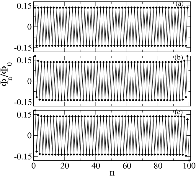
Figure 2: The normalized flux $2\pi\Phi_{n}/\Phi_{0}$ vs plaquette number $n$, for (a) a periodic array ($N=100$); (b) an open-ended array with even $N$ ($N=100$); (c) an open-ended array with odd $N$ ($N=101$). $I_{c0}=I_{c\pi}$, and $k=0.8$.

For a finite array with $N$ total number of JJs, $n=1,2,...,N$. The earlier equations may also be obtained by applying Kirchhoff laws in the equivalent electrical circuit Watanabe , where each single JJ is described by the resistively and capacitively shunted junction (RCSJ) model. In this model the JJ consists of a capacitive branch, a resistive branch, and a superconducting branch, all connected in parallel.

Equations (II) are written in the standard normalization form, i.e. $a=D/\lambda_{j}$ is normalized to $\lambda_{j}$ with $D$ being the spatial separation of neighbouring JJs, the temporal variable $t$ to the inverse plasma frequency $\omega_{p}^{-1}$, and $\gamma=I_{c}/I_{c0}$ is normalized to $I_{c0}$. Then, $I_{c0}=1$ in equations (II), and $I_{c\pi}$ actually represents the ratio $I_{c\pi}/I_{c0}$. The voltage $V_{n}$ across the $n-$th JJ is normalized so that $v_{n}=V_{n}/V_{p}$ where $V_{p}=\Phi_{0}\omega_{p}/(2\pi)$, and $\Phi_{0}=h/(2e)$ is the flux quantum (with $h$ and $e$ being the Planck’s constant and the electron charge, respectively). Equation (II) is analogous to that deduced in reference Goldobin in the context of analysis of zig-zag arrays Smilde . Below we deal with arrays both with periodic and open ends, i.e., annular and linear finite arrays, respectively. Then, in both cases, the governing equations (II) remain the same for $n=2,...,N-1$. The same equations are also valid at the end points $n=1$ and $n=N$, if we define artificial phases $\phi_{0}$ and $\phi_{N+1}$ such that

$$\phi_{0}(t)=\phi_{N}(t)-2\pi M_{f}\qquad\phi_{N+1}(t)=\phi_{1}(t)+2\pi M_{f},$$ (7)

for periodic boundary conditions (e.g., Watanabe ; Pfeiffer ), and

$$\phi_{0}(t)=\phi_{1}(t)\qquad\phi_{N+1}(t)=\phi_{N}(t),$$ (8)

for open-ended boundary conditions. The integer $M_{f}$ in equation (7) is the number of $2\pi$ fluxons trapped in the annular array.

Equations (II) are integrated with a standard fourth order Runge - Kutta algorithm with fixed time-stepping (typically $0.01$). In figure 2 we plot the calculated normalized flux $\Phi_{n}/\Phi_{0}=(\phi_{n}-\phi_{n+1})/(2\pi)$ in each elementary cell (plaquette) as a function of the junction number $n$, for three different arrays in their ground state: a periodic array (figure 2(a)), and open-ended arrays with even and odd $N$ (figures 2(b) and 2(c), respectively). In the former case the flux clearly alternates between two values of opposite sign and the same magnitude, the latter depending on the coupling constant $k$, indicating that the flux lattice is actually periodic with a period of two elementary cells. We can thus define a new extented unit cell, with respect to the flux periodicity, which consists of two elementary cells. Then, we can evaluate the (normalized) average flux in each of the extended cells, $\Phi_{pm}=(\Phi_{2m-1}+\Phi_{2m})/(2\Phi_{0})$, where $m=1,...,N/2$ numbers the extended cell composed of the ($2m-1$)th and $2m$th elementary cells. Clearly, $\Phi_{pm}$ vs $m$ is a constant which equals to zero. The same remarks also hold for the open-ended arrays, both with even and odd $N$, relatively far from the end JJs.

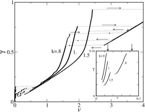
Figure 3: Current-voltage characteristics for an array with $N$ even ($N=100$), $I_{c0}=I_{c\pi}$, $\alpha=0.2$ and $k$ as shown in the figure. The arrows along the dotted lines indicate the direction of the jumps. Inset: half-integer ZF-like steps in the lower-voltage part of the curves shown in main figure. The vertical arrows indicate the position of $v_{m}$ for ZFS1/2 and ZFS3/2 for $k=0.8$ (see text).

III Current - voltage characteristics and zero-field-like steps

For obtaining the current-voltage ($\gamma-v$) characteristics for an open-ended array, we initialize the system with $\phi_{n}=0$ and $\pi$ for $n$ odd and even, respectively, and $\dot{\phi}_{n}=0$ for any $n$ at $t=0$ and $\gamma=0$. (The overdot denotes derivation with respect to the temporal variable.) Then equations (II) are integrated forward in time up to $t_{1}=1000$, by which time the system has reached a steady state. We then calculate the time averaged voltage $v_{n}$ across each JJ by averaging over an additional $t_{2}-t_{1}$ dimensionless time-units, i.e., $v_{n}=\frac{1}{t_{2}-t_{1}}\int_{t_{1}}^{t_{2}}\dot{\phi}_{n}\,dt$, where $t_{2}=2000$. The voltage of the array $v$ is obtained by averaging over all JJs, i.e., $v=\sum_{n=1}^{N}v_{n}/N$. The dc bias $\gamma$ is then increased by $\delta\gamma$ and the calculation is repeated, assuming as initial condition the steady state achieved in the previous calculation. We continue this procedure increasing $\gamma$ by $\delta\gamma$ until $\gamma=1.1$, then decrease $\gamma$ with same steps back to zero, obtaining the $\gamma-v$ characteristics shown in figures 3 and 4 for even $N$(=100) and odd $N$(=101), respectively ($\delta\gamma=0.005$ for the curves in the main figures and $0.001$ for the curves in the insets). Large hysteresis is observed in the high-voltage part ($v\stackrel{{\scriptstyle>}}{{\sim}}0.5$) of all characteristics in both figures, even though the damping coefficient is rather high ($\alpha=0.2$). Small hysteretic effects are also apparent in the low-voltage parts (not shown for clarity). Apparently, the high-voltage characteristics in figures 3 and 4 for same $k$ are practically the same. The solutions on the high voltage branches have been discussed in detail in reference Chandran , and it seems that they are not significantly affected by the choice of boundary conditions. Here, we focus on the the low-voltage parts of those characteristics, which exhibit significant quantitative differences for odd and even $N$.

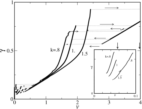
Figure 4: Current-voltage characteristics for an array with $N$ odd ($N=101$), $I_{c0}=I_{c\pi}$, $\alpha=0.2$ and $k$ as shown in the figure. The arrows along the dotted lines indicate the direction of the jumps. Inset: integer ZF-like steps in the lower-voltage part of the curves shown in main figure. The vertical arrows indicate the position of $v_{m}$ for ZFS1 and ZFS2 for $k=0.8$ (see text).

That can be seen by comparing the insets of figures 3 and 4, which display a magnified portion of the corresponding low-voltage characteristics seen in the main figures. There we can see the appearence of current steps, similar with those observed in $0-$JJ arrays (see for example references Ustinov1 ; Pfeiffer ). Those steps are the discrete counterparts of the zero-field steps (ZFSs) appearing in the $\gamma-v$ characteristics of continuous, long $0-$JJ, due to fluxon resonant motion. In this case the propagating fluxons are $2\pi-$kinks and their multitudes, while single $\pi-$kinks are unstable. In a continuous, long $0-$JJ, with equivalent normalized length $L\simeq Na$, the normalized voltage at maximum fluxon velocity $v_{m}$ of the first ZFS would be $v_{m}=2\pi/L\simeq 0.056$ for $k=0.8$. Thus, the first half-integer ZFS (ZFS1/2) would have $v_{m}=0.028$, while the second integer ZFS (ZFS2) and second half-integer ZFS (ZFS3/2) would have $v_{m}=0.112$ and $0.084$, repectively. The fluxon width decreases (i.e., the fluxon size contracts) with increasing velocity. Thus, in the discrete system, a fluxon cannot reach the maximum velocity of its continuous counterpart, since its contracted size cannot be smaller than $a$. In each of the insets in figures 3 and 4 there are two ZFS-like branches with $k=0.8$, with maximum $v$ (defined at the top of the steps) equal to $0.024$, $0.072$, and $0.048$, $0.093$, respectively. Thus, the steps in the inset of figure 3 can be identified with the discrete counterparts of half-integer ZFSs (namely with ZFS$1/2$ and ZFS$3/2$), while those in the inset of figure 4 with the discrete counterparts of integer ZFSs (ZFS$1$ and ZFS$2$).

Figure 5: An instantaneous profile of (a) $\Phi_{n}/\Phi_{0}$ vs $n$, and (b) $\Phi_{pm}$ vs. extended cell number $m$, for $I_{c0}=I_{c\pi}$, $N=100$, $\gamma=0.2$, $k=0.8$, and $\gamma=0.13$ on the ZFS$1/2-$like branch in the inset of figure 3.

Inspection of the time evolution of the phases (not shown) reveals that the ZFS$1/2$-like branch for even $N$(=100) is due to a $\pi-$kink propagating in the array, on a staggered phase background. In figure 5 we show the instantaneous profile of the normalized flux as a function of the plaquette number $n$, and $\Phi_{pm}$ as a function of the number of the extended cell $m$, for $\gamma=0.13$. The antiferromagnetic background in the flux (figure 5(a)) obscures the picture, but its proper elimination with the doubling of the unit cell along with the definition of $\Phi_{pm}$ makes things more clear (figure 5(b)). Then, in figure 5b we see clearly the discrete $\pi-$kink in a form which is the discrete counterpart of the spatial phase derivative in continuous systems. Also apparent they are small oscillations behind the $\pi-$kink, a phenomenon known from $0-$JJ arrays Ustinov1 ; Pfeiffer , where moving $2\pi-$kinks excite linear oscillating modes of the array (Cherenkov radiation). Those oscillations, however, get strongly damped and die out fast away from the kink. In figure 6 the same quantities for an array with the same parameters but odd $N$(=101) are plotted for $\gamma=0.13$ on the ZFS$1$-like branch. Here we always have a $\pi-$kink and a $\pi-$antikink pair. Cherenkov radiation is also apparent here (figure 6(b)) behind both the propagating $\pi-$kinks.

Figure 6: A snapshot of (a) $\Phi_{n}/\Phi_{0}$ vs $n$, and (b) $\Phi_{pm}$ vs. extended cell number $m$, for $I_{c0}=I_{c\pi}$, $N=101$, $\gamma=0.2$, $k=0.8$, and $\gamma=0.13$ on the ZFS$1-$like branch in the inset of figure 4.

Inserting one (or more) $2\pi-$kink(s) in both the even and odd $N$ arrays, we get higher order ZFS-like branches. The ZFS$3/2$- and ZFS$2$-like branches for even and odd $N$, respectively, are shown in the insets of figure 3 and 4, respectively (only for $k=0.8$). Those branches were obtained by inserting one $2\pi-$kink in the arrays. Again, inspection of the phases reveals that the $2\pi-$kink is fractionalized into two closely spaced but clearly separated $\pi-$kinks which, however, are not identical. The snapshot in figure 7 shows the normalized flux as a function of the plaquette number $n$, and $\Phi_{pm}$ as a function of the number of the extended cell $m$, for $\gamma=0.13$ on the ZFS$3/2$-like branch in the inset of figure 3 ($N=100$, even). The fractionalized $2\pi-$kink at the right of figure 7(b), now coexists with the single $\pi-$kink in the array. The corresponding figure (figure 8) for the ZFS$2$-like branch in the inset of figure 4 ($N=101$, odd), shows the fractionalized $2\pi-$kink along with a $\pi-$kink - $\pi-$antikink pair.

The direction of motion of the fractionalized $2\pi-$kinks depends on their polarity when they are inserted in the array. These kinks, either the single one or the ones obtained by fractionalization, behave in many aspects like the usual $2\pi-$kinks. They get reflected by the ends changing their polarity, and interact completelly elastically, passing the one through the other without any apparent shape change. Although not shown in figures 3 and 4, the depinning current $\gamma_{c}$ related to the Peierls-Nabarro potential, which the kink should overcome in order to start moving, is practically the same for $N$ even and odd. It increases with increasing discreteness (decreasing $k$), having the values $\gamma_{c}=0.123,~{}0.099$ and $0.066$ for $k=0.8,~{}1.0$ and $1.5$, respectively. The fractionalized $2\pi-$kinks shown for a specific illustrative case in the figures 7(b) and 8(b), are closely spaced and they move together in the same direction without changing their distance of separation. Thus, they essentially form a single bound state which resembles the bunched fluxon state observed in $0-$JJ arrays Ustinov2 . Such a state results from strong interactions between kinks, which is mediated by their Cherenkov ”tails”. As a result, the Cherenkov radiation behind the bunched state is strongly suppressed, which is exactly what we observe in our figures 7(b) and 8(b).

Figure 7: A snapshot of (a) $\Phi_{n}/\Phi_{0}$ vs $n$, and (b) $\Phi_{pm}$ vs. extended cell number $m$, for $I_{c0}=I_{c\pi}$, $N=100$, $\gamma=0.2$, $k=0.8$, and $\gamma=0.13$ on the ZFS$3/2-$like branch in the inset of figure 3.

Figure 8: A snapshot of (a) $\Phi_{n}/\Phi_{0}$ vs $n$, and (b) $\Phi_{pm}$ vs. extended cell number $m$, for $I_{c0}=I_{c\pi}$, $N=101$, $\gamma=0.2$, $k=0.8$, and $\gamma=0.13$ on the ZFS$2-$like branch in the inset of figure 4.

In annular $0-\pi$ JJ arrays with both even and odd $N$, which satisfy the boundary conditions (7), the effect of fractionalization of $2\pi-$fluxons also appears Chandran . In that case, $2\pi-$fluxons can be inserted in the array either by setting $M_{f}$ to a nonzero integer value or by an appropriate initial condition. For both even and odd $N$ and a nonzero dc bias $\gamma$ (e.g., $\gamma=0.13$), there is a number of $\pi-$kinks and $\pi-$antikinks moving along the array such that the total flux is always an integer as required by the boundary conditions. They appear either as $\pi-$kink - $\pi-$antikink pairs moving in opposite directions, or as two bunched $\pi-$kinks looking very much like those in figures 7 and 8. However, we did not find single $\pi-$kinks in this case, so that half-integer ZF-like branches do not appear. Thus, it seems that half-integer ZF-like branches appear only for arrays with even $N$ satisfying the boundary conditions (8), i.e., for linear arrays. This is probably due to the amount of the net total flux in a $0-\pi$ JJ array in its ground state. For arrays satisfying periodic boundary conditions without inserted flux, with either odd or even $N$, the ground state is always arranged such that the total flux is equal to zero. Apparently, this is not always the case for open-ended boundary conditions. For odd $N$ there is an even number of elementary cells in the array, so that the contributions from all cells exactly cancel, resulting in zero total flux. However, for even $N$ there is an odd number of elementary cells in the array, and the total flux attains a nonzero value (approximatelly equal to $0.274$ in figure 2(b)). With increasing bias current above the Peirls-Nabarro barrier, that ground state becomes unstable against the formation of a $\pi-$kink. Dynamic simulations for such $0-\pi$ JJ arrays with periodic boundary conditions have been performed in reference Chandran , where it was shown that $2\pi-$kinks fractionalize into a pair of $\pi-$kinks in certain regions of $k-I_{cp}$ space. However, ZF-like steps on the current - voltage characteristics are not discussed. Although a $0-\pi$ JJ array is still hypothetical, it can be possibly realized with the existing technology. Moreover, it has been argued Kornev2 that bicrystal grain boundary JJs with $45^{o}$ misorientations angle, form intrinsically an array of alternatingly $0$ and $\pi$ contacts. In this context, a discrete array of alternating $0-$ and $\pi-$JJs has been used as a model to study the dynamics as well as the magnetic field dependence of such JJs Kornev2 ; Kornev .

IV Conclusions

In conclusion, we caclulated numerically the $\gamma-v$ characteristics for a 1D discrete, planar array of small, parallel connected alternating $0-$ and $\pi-$JJs, which exhibit current steps in the low-voltage part. For even $N$, the maximum voltage of the steps (evaluated at the top of each step) is approximately two times smaller than the maximum voltage of the steps for odd $N$. Comparison with the continuous long JJ, helps in identifying those steps as half-integer and integer ZFS-like steps for even and odd $N$, respectively. Inspection of the phases and the fluxes reveals that in both cases the system supports $\pi-$kinks, either a single $\pi-$kink or a $\pi-$kink - $\pi-$antikink pair for even and odd $N$, respectively, which can propagate in the array. Moreover, any $2\pi-$kink inserted in the array is fractionalized into two, generally different $\pi-$kinks, which propagate together in the array along with the single $\pi-$kink or the $\pi-$kink - $\pi-$antikink pair, for even and odd $N$, respectively, giving rise to higher order half-integer and integer ZFS-like branches. In the continuum, half-integer ZFSs have been observed experimentally in not very long $0-\pi$ JJs due to the hopping of the semifluxons Goldobin2 . Similar ZFS-like branches can be found in rather wide parameter range. The case with $k=0.8$, for which the system is already highly discrete, was chosen only for better illustration of the half-integer ZFSs. Those steps can also be found even for low damping (i.e., $\alpha=0.02$), as well as for higher damping (i.e., $\alpha=0.42$), which is more appropriate for high-temperature superconductor JJ arrays Smilde . Also, they may exist even for slightly different critical currents (i.e., for $I_{c\pi}=0.9$ for even $N$). Dynamic states such as those described above could in principle be detected by low-temperature scanning electron microscopy (LTSEM) imaging Doderer .

References

- (1) Bulaevskii L N, Kuzii V V and Sobyanin A A 1977 Pis’ma Zh. Éksp. Teor. Fiz. 25 314 [1977 JETP Lett. 25 290].
- (2) Ryazanov V V, Oboznov V A, Rusanov A Yu, Veretennikov A V, Golubov A A and J. Aarts J 2001 Phys. Rev. Lett. 86 2427
- (3) Kontos T, Aprili M, Lesueur J, Genêt F, Stephanidis B and Boursier R 2002 Phys. Rev. Lett. 89 137007
- (4) Radović Z, Lazarides N and Flytzanis N 2003 Phys. Rev. B 68 014501
- (5) Lombardi F, Tafuri F, Ricci F, Miletto Granozio F, Barone A, Testa G, Sarnelli E, Kirtley J R and C. C. Tsuei 2002 Phys. Rev. Lett. 89 207001
- (6) Testa G, Monaco A, Esposito E, Sarnelli E, Kang D-J, Tarte E J, Mennema S H and Blamire M G, 2003 cond-mat/0310727
- (7) Weides M, Kemmler M, Kohlstedt H, Waser R, Koelle D, Kleiner R and Goldobin E 2006 Phys. Rev. Lett. 97 247001
- (8) Weides M, Schindler C and Kohlstedt H 2007 J. Appl. Phys. 101 063902
- (9) Ustinov A V Physica D 123 315
- (10) Pedersen N F and Ustinov A V 1995 Supercond. Sci. Technol. 8 389 and references therein.
- (11) O. M. Brown, and Y. S. Kivshar, 1998 Phys. Rep. 306 1
- (12) Ustinov A V, Cirillo M, Larsen B H, Oboznov V A, Carelli P and G. Rotoli G 1995 Phys. Rev. B 51 3081 and references therein.
- (13) Nakajima K, Sugahara H, Fujimaki A and Sawada Y 1989 J. Appl. Phys. 66 949
- (14) Buchholz F-Im and Kessel W 1999 Physica C 326-327 111
- (15) Schultze V, IJsselsteijn R, Boucher R, Meyer H-G, Oppenländer J, Häussler Ch and Schopohl N 2003 Supercond. Sci. Technol. 16 1356
- (16) Shi S C, Wang M J and Noguchi T 2002 Supercond. Sci. Technol. 15 1717
- (17) Kaplunenko V and Fischer G M 2004 Supercond. Sci. Technol. 17 S145
- (18) Ustinov A V and Kaplunenko V K 2003 J. Appl. Phys. 94 5405
- (19) Balashov D, Dimov B, Khabipov M, Ortlepp T, Hagedorn D, Zorin A B, Buchholz F-I, Uhlmann F H and Niemeyer J 2007 IEEE Trans. Appl. Supercond. 17 142
- (20) Ryazanov V V, Oboznov V A, Timofeev A V and Bol’ginov V V 2003 Microelectron. Eng. 69 341
- (21) De Leo C and Rotoli G 2002 Supercond. Sci. Technol. 15 1711
- (22) Liu D T, Zhu X M, Tian Y, Zhao S P and Chen G H 2005 Supercond. Sci. Technol. 18 1539
- (23) Tian Ye, Wang H W, Kong X Y, Zhao S P, Chen G H and Yang Q S 2004 Supercond. Sci. Technol. 17 838
- (24) Kornev V K, Klenov N V, Oboznov V A, Feofanov A K, Bol’ginov V V, Ryazanov V V and Pedersen N F 2004 Supercond. Sci. Technol. 17 S355
- (25) Caputo J G and Loukitch L 2005 Physica C 425 69
- (26) Rotoli G 2003 Phys. Rev. B 68 052505
- (27) Kornev V K, Borisenko I V, Mozhaev P B, Ovsyannikov G A and Pedersen N F 2002 Physica C 367 285.
- (28) Kornev V K, Soloviev I I, Klenov N V, Pedersen N F, Borisenko I V, Mozhaev P B and Ovsyannikov G A 2003 IEEE Trans. Appl. Supercond. 13 825
- (29) Rotoli G 2005 IEEE Trans. Appl. Supercond. 15 852
- (30) Li Z-Z, Feng Y, Wang F-R and Dai Y-D 2007 Chinese Physics 16 1450
- (31) Chandran M and Kulkarni R V 2003 Phys. Rev. B 68 104505
- (32) Susanto H, Darminto and van Gils S A 2007 Phys. Lett. A 361 270
- (33) Mints R G 1998 Phys. Rev. B 57 R3221
- (34) Il’ichev E, Zakosarenko V, IJsselsteijn R P J, Hoenig H E, Meyer H-G, Fistul M V and Müller P 1999 Phys. Rev. B 59 11502
- (35) Lindström T, Johansson J, Bauch T, Stepantsov E, Lombardi F and Charlebois S A 2006 Phys. Rev. B 74 014503
- (36) Watanabe S, van der Zant H S J, Strogatz S H and Orlando T P 1996 Physica D 97 429
- (37) Goldobin E, Koelle D and Kleiner R 2002 Phys. Rev. B 66 100508
- (38) Smilde H J H, Ariando, Blank D H A, Gerritsma G J, Hilgenkamp H and Rogalla H 2002 Phys. Rev. Lett. 88 057004
- (39) Pfeiffer J, Schuster M, Abdumalikov A A, Jr. and Ustinov A V 2006 Phys. Rev. Lett. 96 034103
- (40) Ustinov A V, Malomed B A and Sakai S 1998 Phys. Rev. B 57 11691
- (41) Goldobin E, Sterck A, Gaber T, Koelle D and Kleiner R 2004 Phys. Rev. Lett. 92 057005
- (42) Doderer T, Kaplunenko V K, Mygind J and Pedersen N F 1995 Phys. Rev. B 50 7211