SZ and CMB reconstruction using Generalized Morphological Component Analysis

Abstract

In the last decade, the study of cosmic microwave background (CMB) data has become one of the most powerful tools to study and understand the Universe. More precisely, measuring the CMB power spectrum leads to the estimation of most cosmological parameters. Nevertheless, accessing such precious physical information requires extracting several different astrophysical components from the data. Recovering those astrophysical sources (CMB, Sunyaev-Zel’dovich clusters, galactic dust) thus amounts to a component separation problem which has already led to an intense activity in the field of CMB studies. In this paper, we introduce a new sparsity-based component separation method coined Generalized Morphological Component Analysis (GMCA). The GMCA approach is formulated in a Bayesian maximum a posteriori (MAP) framework. Numerical results show that this new source recovery technique performs well compared to state-of-the-art component separation methods already applied to CMB data.

Introduction

Investigating Cosmic Microwave Background (CMB) data is of huge scientific importance as it improves our knowledge of the Universe [8]. Indeed, most cosmological parameters can be derived from the study of CMB data. In the last decade several experiments (Archeops, Boomerang, Maxima, WMAP - [1]) have already provided large amounts of data and astrophysical information. The forthcoming Planck ESA mission will provide new accurate data requiring effective data analysis tools. More precisely, recovering useful scientific information requires disentangling in the CMB data the contribution of several astrophysical components namely CMB itself, Galactic emissions from dust and synchrotron, Sunyaev-Zel’dovich (SZ) clusters [12] to name a few. In the frequency range used for CMB observations [3], the observed data combines contributions from distinct astrophysical components the recovery of which falls in the frame of component separation.
Following a standard practice in the field of component or source separation, which has physical grounds here, the observed sky is modeled as a linear mixture of statistically independent components. The observation with detector $i$ is then a noisy linear mixture of $n$ independent sources $\{s_{j}\}_{j=1,\cdots,n}$ : $x_{i}=\sum_{j=1}^{n}a_{ij}s_{j}+n_{i}$. The coefficient $a_{ij}$ reflects the emission law of source $s_{j}$ in the frequency band of the $i$-th sensor; $n_{i}$ models instrumental noise. When $m$ sensors provide observations at different frequencies, this linear mixture model can be rewritten in a more convenient matrix formulation :

$${\bf X}={\bf AS}+{\bf N}$$ (1)

where ${\bf X}$ is the $m\times t$ data matrix the rows of which are the observed data maps in each channel, ${\bf A}$ is the $m\times n$ mixing matrix, ${\bf S}$ is the $n\times t$ source matrix the rows of which are the sources $s_{j}$, and ${\bf N}$ is the $m\times t$ noise matrix. In practice, both the sources ${\bf S}$ and their emission laws ${\bf A}$ may be unknown or only partly known. A component separation technique then aims at estimating both ${\bf S}$ and ${\bf A}$ from the data ${\bf X}$. This problem refers to Blind Source Separation (BSS).
Amongst all the physical components mixed in the observed data, each one raises scientific interest. Thus it would be worthwhile to devise a separation technique able to differentiate effectively between most physical components. Up to now, several source separation techniques have already been used in the field of CMB data studies. In this paper, we concentrate on two particular components: the CMB and the SZ components. For such processes, state-of-the-art blind separation methods used on CMB data are:

• JADE which is a classical Independent Component Analysis technique based on fourth order statistics. Its effectiveness at extracting non-Gaussian components such as the SZ map was shown in [10].

• Spectral Matching ICA (SMICA) (see [5] and [9]) has been devised to accurately separate the CMB component. SMICA assumes the case of mixed stationary Gaussian components in a noisy environment. It is based on second order statistics. In the Fourier representation, colored stationary Gaussian components are discernible based on the diversity of their power spectra. SMICA is then well adapted to Gaussian components such as CMB.

Neither of the aforementioned techniques is able to effectively extract both the SZ and CMB maps. In this paper we propose a novel sparsity-based component separation technique coined Generalized Morphological Component Analysis (GMCA) which turns out to be well suited for the recovery of CMB and SZ components. Section 1 describes the GMCA model and the algorithm proposed to solve the corresponding optimization problem. Numerical experiments are given which illustrate the astounding performances of GMCA for CMB and SZ extraction in Section 2. Finally, we show in Section 2.2 that GMCA is versatile enough to account for physical priors.

1 Generalized Morphological Component Analysis

1.1 The GMCA model

In the previous section, we introduced the linear mixture model in Equation 1. We further assume that all the protagonists of the model in Equation 1 are random components (variables or vectors). More particularly, the entries of the noise matrix ${\bf N}$ are assumed to be independently distributed according to a zero mean Gaussian distribution with variance $\sigma_{i}^{2}$ depending on the detector. From physical considerations, ${\bf N}$ models instrumental noise the level of which varies independently from one detector to another. ${\bf N}$ is thus a random Gaussian variable with zero mean and covariance matrix ${\bf\Gamma_{N}}=\mbox{diag}(\sigma_{1}^{2},\cdots,\sigma_{m}^{2})$. In practice, as the detectors are assumed to be accurately calibrated, ${\bf\Gamma_{N}}$ is known with high precision. The log-likelihood function is then the following one :

$$\log P({\bf X}\big{|}{\bf A},{\bf S},{\bf\Gamma_{N}})=-\frac{1}{2}\|{\bf X}-{\bf AS}\|_{2,{\bf\Gamma_{N}}}^{2}+C$$ (2)

where $C$ is a constant. The notation $\|.\|_{2,{\bf\Gamma_{N}}}^{2}$ stands for the Frobenius norm of ${\bf Y}$ in the noise covariance metric : $\|Y\|_{2,{\bf\Gamma_{N}}}^{2}=\mbox{ Trace}\left({\bf Y}^{T}{\bf\Gamma_{N}}^{-1}{\bf Y}\right)$. From a Bayesian point of view, adding physical priors should help the separation task. We first assume no particular knowledge about the emission laws of the components modeled by ${\bf A}$. For simplicity, we consider that each entry of the mixing matrix ${\bf A}$ is i.i.d. from a uniform zero mean distribution. Note that it would be possible to add some physical constraint on the emission laws reflected in ${\bf A}$.
In the general case, source separation is merely a question of diversity and contrast between the sources (see [4]). For instance, on the one hand JADE relies on non-Gaussianity to distinguish between the sources. On the other, SMICA takes advantage of the diversity of the mixed components’ power spectra to achieve the separation task. “Non-Gaussianity” and “power spectra diversity” are contrasts between the sources. A combination of both characteristics, “Non-Gaussianity” and “power spectra diversity”, was also proposed to separate CMB from kinetic SZ signal which are otherwise undistinguishable [7]. Recent work has already emphasized on sparsity as a source of diversity to improve component separation (see [14] and [2]). In that setting, each source $\{s_{j}\}_{j=1,\cdots,n}$ is assumed to be sparse in a representation (potentially overcomplete) $\mathcal{D}$. Formally, $\mathcal{D}$ is a fixed dictionary of signal waveforms written as a $T\times t$ matrix. We define the set of projection coefficients $\alpha_{j}$ such that : $\forall j\in\{1,\cdots,n\},\quad s_{j}=\alpha_{j}\mathcal{D}$. Any source $s_{j}$ is said to be sparse in $\mathcal{D}$ if most of the entries of $\alpha_{j}$ are nearly zero and only a few have “significant” amplitudes. When $\mathcal{D}$ is overcomplete ($T>t$), $\mathcal{D}$ is called a dictionary. The attractiveness of overcomplete representations in image processing theory resides in the potentially very sparse representations that they make possible (see e.g. [6] and references therein). In the field of basic source separation we showed in [2] that morphological diversity and sparsity are key properties leading to better separation. We noticed that the gist of sparsity-based source separation methods leans on the rationale : “independent sources are distinctly sparse in a dictionary $\mathcal{D}$”. In that study, we considered the simple case of morphologically different sources : components were assumed to be sparsely represented in different sub-dictionaries. We illustrated that such a sparsity based prior provides a very effective way to distinguish between sources. In the present paper, we focus on a more general setting : the sources can have similar morphologies (i.e. all the sources are sparsely represented over the whole $\mathcal{D}$). When the overcomplete dictionary $\mathcal{D}$ is made of the union of $D$ orthonormal bases (i.e. $\mathcal{D}=\left[\Phi_{1},\cdots,\Phi_{D}\right]$) then each source is modeled as the linear combination of $D$ so-called morphological components (see [11] for details on Morphological Component Analysis) - each morphological component being sparse in a different orthonormal basis $\{\Phi_{1},\cdots,\Phi_{D}\}$:

$$\forall j\in\{1,\cdots,n\},\quad s_{j}=\sum_{k=1}^{D}\varphi_{jk}=\sum_{k=1}^{D}\alpha_{jk}\Phi_{k}$$ (3)

From a statistical viewpoint, we assume that the entries of $\alpha_{jk}=\varphi_{jk}\Phi_{k}^{T}$ are i.i.d. from a Laplacian probability distribution with scale parameter $1/\mu$:

$$P(\varphi_{jk})\propto\exp\left(-\mu\|\varphi_{jk}\Phi_{k}^{T}\|_{1}\right)$$ (4)

where the $\ell_{1}$-norm $\|.\|_{1}$ stands for $\|x\|_{1}=\sum_{p=1}^{t}|x[p]|$ in which $x[p]$ is the $p$-th entry of $x$. In practice, the Laplacian prior is well adapted to model leptokurtic sparse signals. We classically assume that the morphological components are statistically mutually independent : $P({\bf S})=\prod_{j,k}P(\varphi_{jk})$. Estimating the sources ${\bf S}$ is then equivalent to estimating the set of morphological components $\{\varphi_{jk}\}_{j=1,\cdots,n;k=1,\cdots,D}$. In this Bayesian context, we propose to estimate those morphological components $\{\varphi_{jk}\}$ and the mixing matrix ${\bf A}$ from a maximum a posteriori (MAP) leading to the following optimization problem:

$$\left\{\{\hat{\varphi}_{jk}\},{\bf\hat{A}}\right\}=\arg\max_{\{\varphi_{jk}\},{\bf A}}P({\bf X}|{\bf A},\{\varphi_{jk}\},{\bf\Gamma_{N}})\prod_{j,k}P(\varphi_{jk})P({\bf A})$$ (5)

where we further assumed that the morphological components $\{\varphi_{jk}\}$ are independent of ${\bf A}$. Owing to Equations 2 and 4, the mixing matrix ${\bf A}$ and the morphological components $\{\varphi_{jk}\}$ are obtained by minimizing the following negative log a posteriori:

$$\left\{\{\hat{\varphi}_{jk}\},{\bf\hat{A}}\right\}=\arg\min_{\{\varphi_{jk}\},{\bf A}}\|{\bf X}-{\bf AS}\|_{2,{\bf\Gamma_{N}}}^{2}+2\mu\sum_{j=1}^{n}\sum_{k=1}^{D}\|\varphi_{jk}\Phi_{k}^{T}\|_{1}$$ (6)

where $\forall j\in\{1,\cdots,n\},\quad s_{j}=\sum_{k=1}^{D}\varphi_{jk}$. Equation 6 leads to the GMCA estimates of the sources and the mixing matrix in a general sparse component separation context. Interestingly, in the case of CMB data, the sources we look for (CMB, galactic dust and SZ) are quite sparse in the same unique orthonormal wavelet basis. The dictionary $\mathcal{D}$ then reduces to a single orthonormal basis $\Phi$. In that case, since $\Phi$ is unitary, Equation 6 can be rewritten as follows :

$$\left\{{\bf\hat{\alpha}},{\bf\hat{A}}\right\} = \arg\min_{{\boldsymbol{\alpha}},{\bf A}}\|{\bf X}\Phi^{T}-{\bf A\alpha}\|_{2,{\bf\Gamma_{N}}}^{2}+2\mu\|{\boldsymbol{\alpha}}\|_{1}$$ (7)

$$= \arg\min_{{\boldsymbol{\alpha}},{\bf A}}f_{\mu}({\boldsymbol{\alpha}},{\bf A})={\arg\min}_{{\boldsymbol{\alpha}},{\bf A}}f_{0}({\bf A},{\boldsymbol{\alpha}})+2\mu f_{1}({\boldsymbol{\alpha}})$$

where ${\boldsymbol{\alpha}}={\bf S}\Phi^{T}$. Note that the estimation is done in the sparse representation $\Phi$ requiring a single transform of the data ${\bf X}\Phi^{T}$. To remain computationally efficient, GMCA relies on practical transforms which generally involve fast implicit operators (typical complexity of $\mathcal{O}\left(t\right)$ or $\mathcal{O}\left(t\log t\right)$). In [14], the authors also used a unique orthonormal wavelet basis. While a gradient descent is used in [14], we use a fast and efficient iterative thresholding optimization scheme which we describe in the next section.

1.2 Solving the optimization problem

The maximum a posteriori estimates of the coefficients ${\boldsymbol{\alpha}}$ and the mixing matrix in Equation 7 lead to a non-convex minimization problem. Note that in Equation 7 the functional to be minimized suffers from several invariances : any permutation or rescaling of the sources and the mixing matrix leaves the product $\bf A{\boldsymbol{\alpha}}$ unaltered. The scale invariance is computationally alleviated by forcing the columns of ${\bf A}$ to have unit $\ell_{2}$ norm : $\forall i\in{\{1,\cdots,n\}},\quad a^{i^{T}}a^{i}=1$ where $a^{i}$ is the $i$-th column of ${\bf A}$.
As solutions of problem (7) have no explicit formulation, we propose solving it by means of a block-coordinate relaxation iterative algorithm such that each iteration $(h)$ is decomposed into two steps : (i) estimation of the sources ${\bf S}$ assuming the mixing matrix is fixed to its current estimate ${\bf\hat{A}}^{(h-1)}$ and (ii) estimation of the mixing matrix assuming the sources are fixed to their current estimates ${\bf\hat{S}}^{(h)}$. It is not difficult to see that the objective MAP functional in (7) is continuous on its effective domain and has compact level sets. Moreover, this objective function is convex in the source coefficient vectors $(\alpha_{1},\ldots,\alpha_{n})$, and $f_{0}$ has an open domain, is continuous and Gâteaux differentiable. Thus by [13, Theorem 4.1], the iterates generated by our alternating algorithm are defined and bounded, and each accumulation point is a stationary point of the MAP functional. In other words, our iterative algorithm will converge. Hence, at iteration $(h)$, the sources are estimated from a maximum a posteriori assuming ${\bf A}={\bf\hat{A}}^{(h-1)}$. By classical ideas in convex analysis, a necessary condition for ${\boldsymbol{\alpha}}$ to be a minimizer is that the zero is an element of the subdifferential of the objective at ${\boldsymbol{\alpha}}$. We calculate:

$$\partial_{\boldsymbol{\alpha}}f_{\mu}({\boldsymbol{\alpha}},{\bf A})=-2{\bf{\bf A}}^{T}{\bf\Gamma_{N}}^{-1}({\bf X}\Phi^{T}-{\bf A}{\boldsymbol{\alpha}})+2\mu\partial_{\boldsymbol{\alpha}}\|{\boldsymbol{\alpha}}\|_{1}$$ (8)

where $\partial_{\boldsymbol{\alpha}}\|{\boldsymbol{\alpha}}\|_{1}$ is defined as (owing to the separability of the prior):

$$\partial_{\boldsymbol{\alpha}}\|{\boldsymbol{\alpha}}\|_{1}=\left\{U\in\mathbb{R}^{n\times t}\Bigg{|}\begin{array}[]{ccc}U{j,k}&=\mbox{ sign}(\alpha_{j,k}),&~{}\alpha_{j,k}\neq 0\\ U{j,k}&\in[-1,1],&~{}\alpha_{j,k}=0\end{array}\right\}.$$

Hence, Equation 8 can be rewritten equivalently as two conditions leading to the following (proximal) fixed point equation:

$$\begin{array}[]{cc}\hat{\alpha}_{j,k}=0,&\text{if}~{}\left|{\left({\bf A}^{T}{\bf\Gamma_{N}}^{-1}{\bf X}\Phi^{T}\right)}_{j,k}\right|\leq\mu\\ {\bf{\bf A}}^{T}{\bf\Gamma_{N}}^{-1}({\bf X}\Phi^{T}-{\bf A}\hat{\boldsymbol{\alpha}})=\mu\mbox{ sign}\left(\hat{\boldsymbol{\alpha}}\right),&\text{otherwise}.\end{array}$$ (9)

Unfortunately, Equation 9 has no closed-form solution in general. It must be iterated and is thus computationally demanding. Fortunately, it can be simplified when ${\bf A}$ has nearly orthogonal columns in the noise covariance matrix (i.e. ${\bf\hat{A}}^{T}{\bf\Gamma_{N}}^{-1}{\bf\hat{A}}\simeq\mbox{diag}\left({\bf\hat{A}}^{T}{\bf\Gamma_{N}}^{-1}{\bf\hat{A}}\right)$). Let ${\bf C}={\left({\bf\hat{A}}^{T}{\bf\Gamma_{N}}^{-1}{\bf\hat{A}}\right)}^{-1}{\bf A}^{T}{\bf\Gamma_{N}}^{-1}{\bf X}\Phi^{T}$, Equation 9 boils down to the following set of equations $\forall j\in\{1,\cdots,n\}$:

$$\begin{array}[]{ccc}\hat{\alpha}_{j,k}&=0,\quad\text{if}~{}\left|{{\bf C}}_{j,k}\right|\leq\mu^{(h)}\sigma_{j}^{2}\\ \hat{\alpha}_{j}&={\left[{\bf C}\right]}_{j}-\mu\sigma_{j}^{2}\mbox{ sign}\left(\hat{\alpha}_{j}\right),\quad\text{otherwise}.\end{array}$$ (10)

where $[{\bf Y}]_{j}$ is the $j$-th row of ${\bf Y}$. In practice, even if the approximation we make is not strictly valid, such a simplification leads to good computational results. These equations are known as soft-thresholding with threshold $\mu^{(h)}\sigma_{j}^{2}$. We define $\mathrm{ST}_{\delta}(.)$, the soft-thresholding operator with threshold $\delta$. At iteration $(h)$, the sources are thus estimated such that:

$$\hat{\alpha}_{j}^{(h)}=\mathrm{ST}_{\mu^{(h)}\sigma_{j}^{2}}\left(\left[{\bf C}\right]_{j}\right)$$ (11)

The $j$th source is reconstructed as $\hat{s}_{j}^{(h)}=\hat{\alpha}_{j}^{(h)}\Phi$. The mixing matrix ${\bf A}$ is then estimated by a maximum likelihood estimate amounting to a simple least-squares update assuming ${\bf S}$ is fixed. The GMCA algorithm is then described as follows :

1. Set the number of iterations $I_{\max}$ and thresholds $\delta_{j}^{(0)}=\mu^{(0)}\sigma_{j}^{2}$ 2. While each $\mu^{(h)}$ is higher than a given lower bound $\mu_{min}$ (e.g. can depend on the noise variance),     – Proceed with the following iteration to estimate source coefficients ${\boldsymbol{\alpha}}$ at iteration $h$ assuming ${\bf A}$ is fixed:        $\hat{\alpha}_{j}^{(h)}=\mathrm{ST}_{\mu^{(h)}\sigma_{j}^{2}}\left(\left[{\left({\bf\hat{A}}^{T}{\bf\Gamma_{N}}^{-1}{\bf\hat{A}}\right)}^{-1}{\bf\hat{A}}^{T}{\bf\Gamma_{N}}^{-1}{\bf X}\Phi^{T}\right]_{j}\right)$:     – Update $\bf A$ assuming ${\boldsymbol{\alpha}}$ is fixed :        ${\bf\hat{A}}^{(h)}={\bf X}\Phi^{T}{\bf\hat{\boldsymbol{\alpha}}}^{T}\left({\bf\hat{\boldsymbol{\alpha}}}{\bf\hat{\boldsymbol{\alpha}}}^{T}\right)^{-1}$ – Decrease the threshold $\mu^{(h)}$ following a given strategy

Note that the overall optimization scheme is based on an iterative and alternate thresholding algorithm involving a coarse to fine estimation process. Indeed, coarse versions of the sources (i.e. containing the most “significant” features of the sources) are first computed with high values of $\mu^{(h)}$. In the early stages of the algorithm, the mixing matrix is then estimated from the most “significant” features of the sources which are less perturbed by noise. The estimation of ${\bf A}$ and ${\bf S}$ is then refined at each iteration as $\mu^{(h)}$ (and thus the thresholds $\{\mu^{(h)}\sigma_{j}^{2}\}_{j=1,\cdots,n}$) decreases towards a final value $\mu_{min}$. We already used this minimization scheme in [2] where this optimization process provided robustness and helped convergence even in a noisy context. Experiments in Section 2 illustrate that it achieves good results with GMCA as well.

2 Application to CMB and SZ reconstruction

2.1 Blind component separation

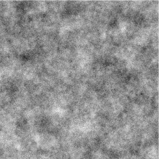
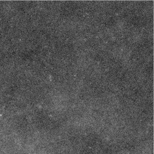
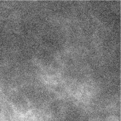
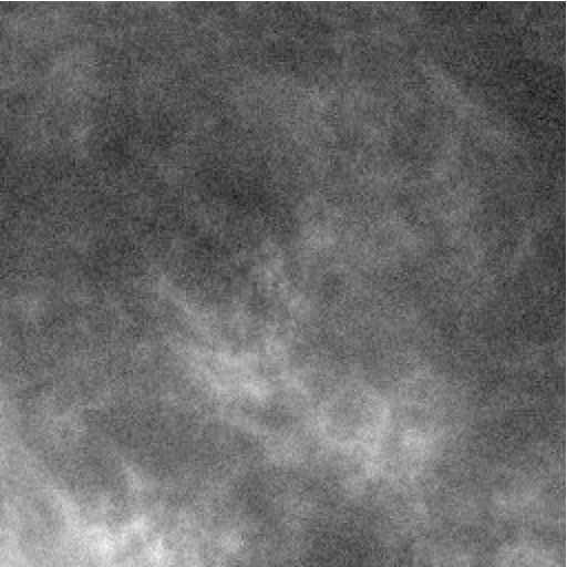
The method described above was applied to synthetic data composed of $m=6$ mixtures of $n=3$ sources : CMB, galactic dust emission and SZ maps illustrated in Figure 1 and 2. Following [5] and [9], we do not take into account the emission at high frequency from the fluctuations of infra-red galaxies.

Figure 1: The simulated sources - Left: CMB. Middle: galactic dust emission. Right: SZ map.

Figure 2: The observed CMB data - global SNR = 2.7dB

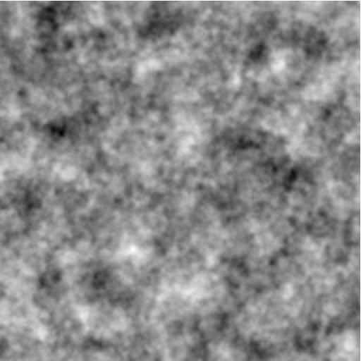
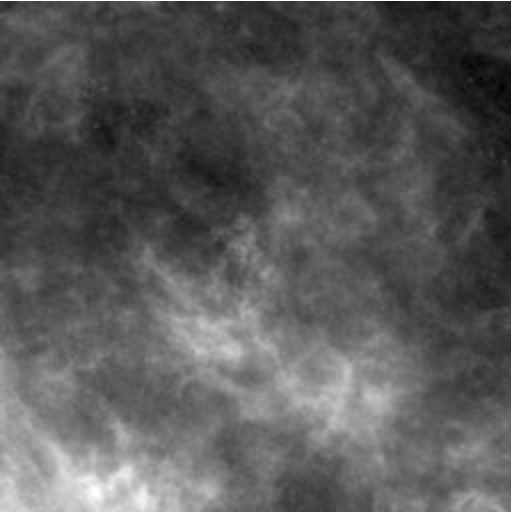
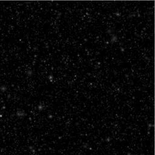
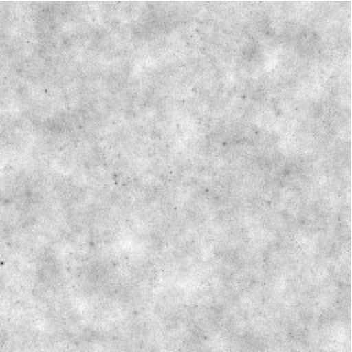
The synthetic data mimic the observations that will be acquired in the six frequency channels of Planck-HFI namely : $100,143,217,353,545$ and $857$ GHz, as shown on Figure 2. White Gaussian noise ${\bf N}$ is added with diagonal covariance matrix ${\bf\Gamma_{N}}$ reflecting the foreseen Planck-HFI noise levels. Experiments were led with $7$ global noise levels with SNR from $1.7$ to $16.7$dB such that the experimental noise covariance $\Gamma_{\bf N}$ was proportional to the nominal noise covariance. Note that the nominal Planck-HFI global noise level is about $10$dB. Each measurement point was computed from $30$ experiments involving random noise, randomly chosen sources from a data set of several simulated CMB, galactic dust and SZ $256\times 256$ maps. The astrophysical components and the mixture maps were generated as in [9] according to equation (1) based on model or experimental emission laws, possibly extrapolated, of the individual components. Separation was obtained with GMCA using a single orthonormal wavelet basis. Figure 3 depicts the average correlation coefficients over experiments between the estimated source maps and the true source maps.

Figure 3: Left Column : Mean value of the correlation coefficients between the estimated source map and the true source map - Right Column : Dispersion of these correlation coefficients : First line : CMB. Second line: galactic dust. Third line: SZ map. Fourth line: mixing matrix criterion $\Delta_{\bf A}$ Legend : JADE : dotted line with $\Box$ - SMICA : dashed line with $\circ$ - GMCA : solid line. Abscissa : SNR in dB.

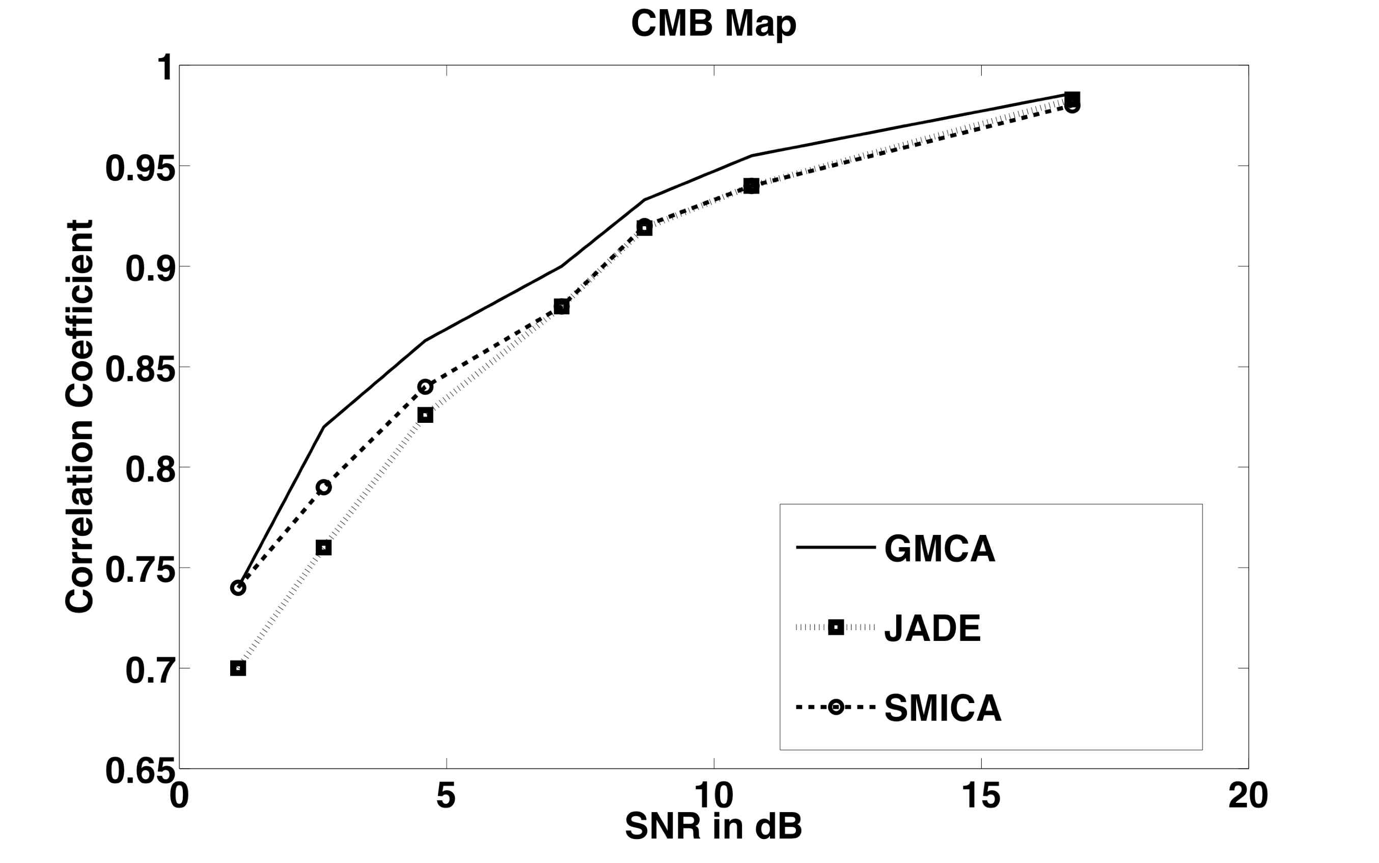
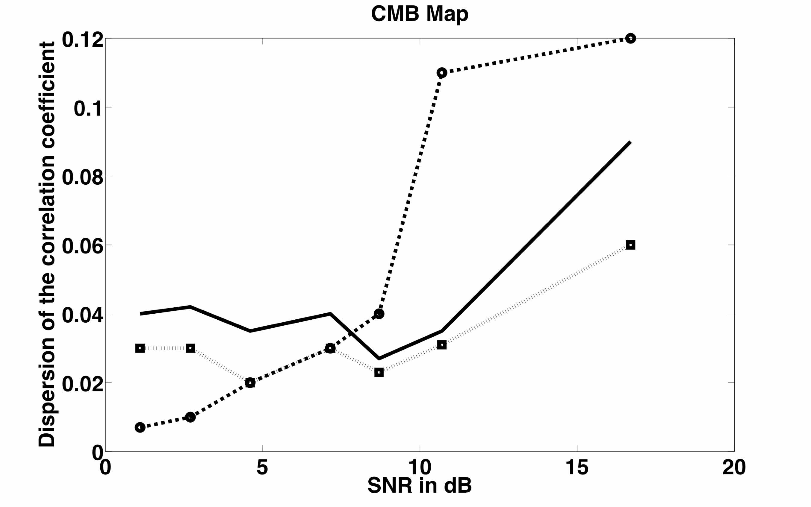
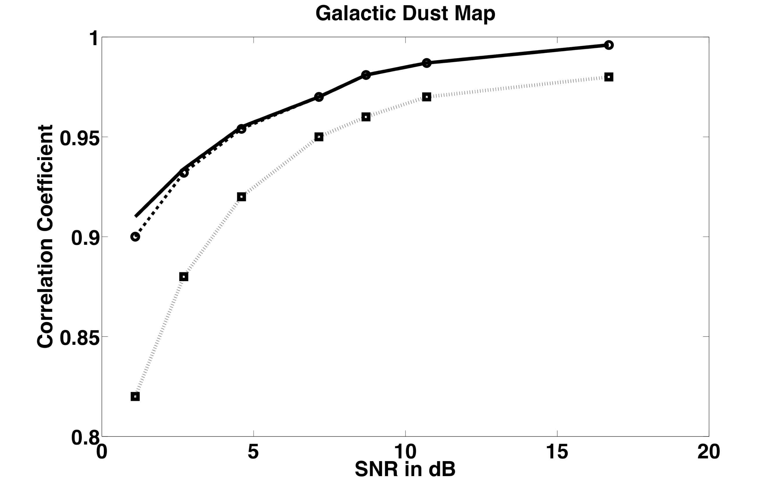
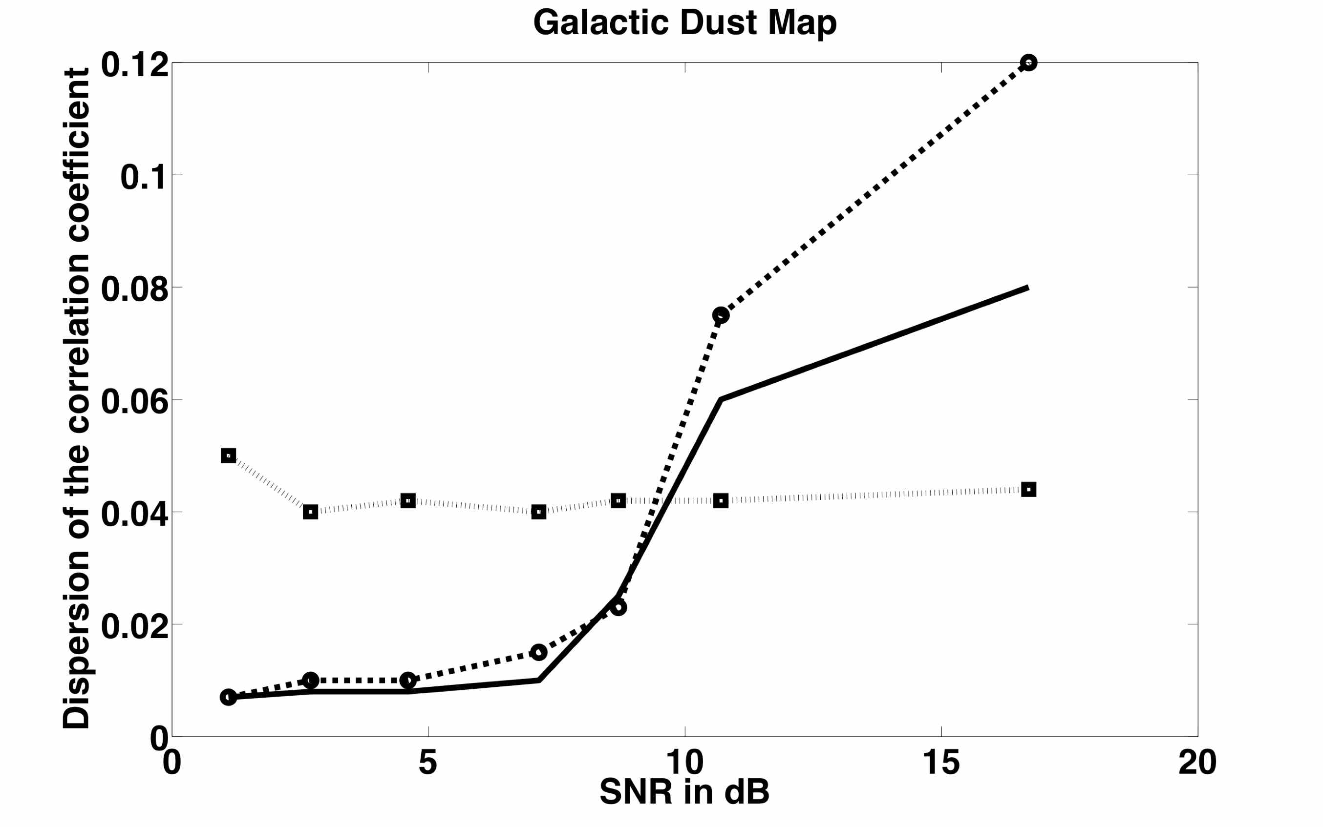
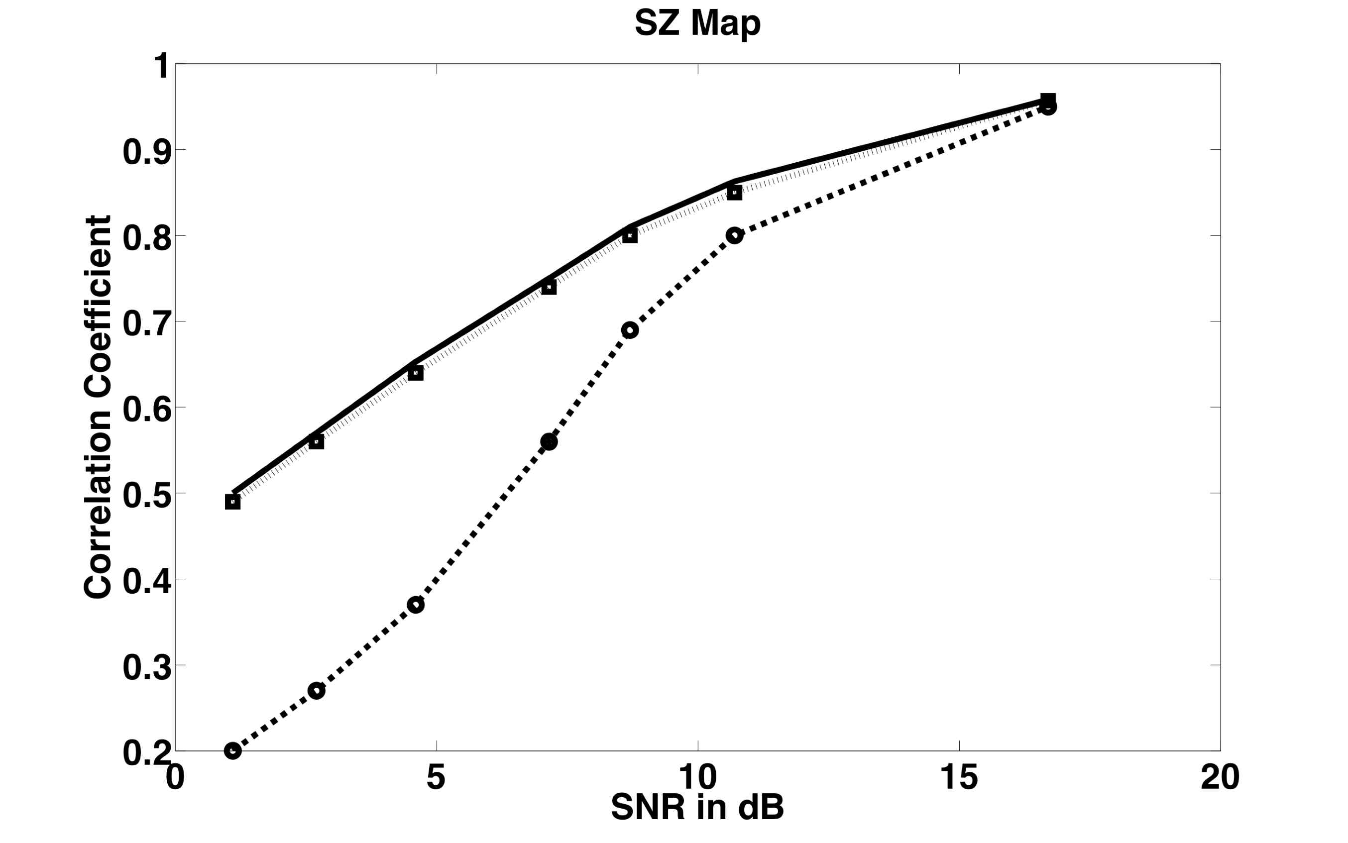
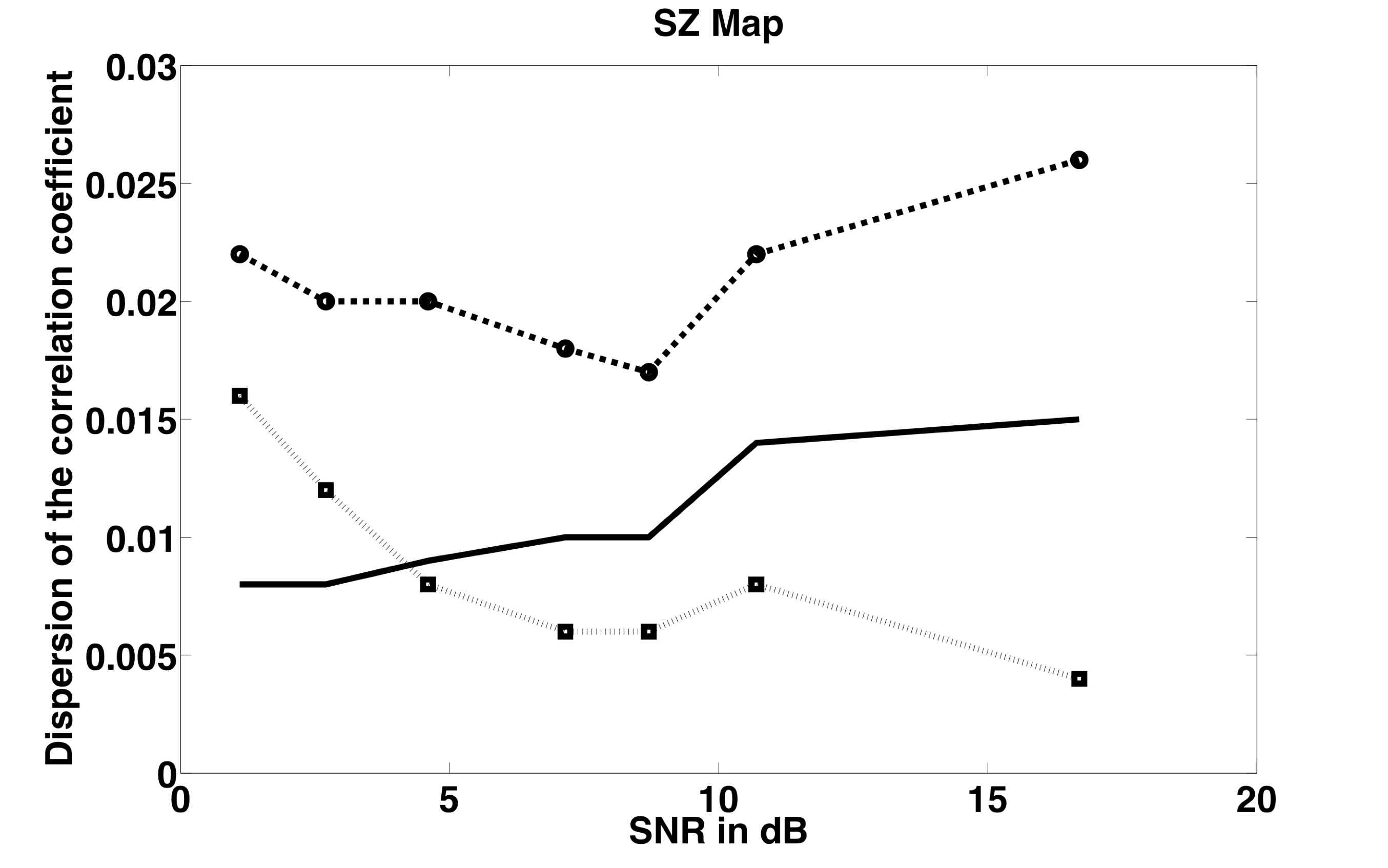
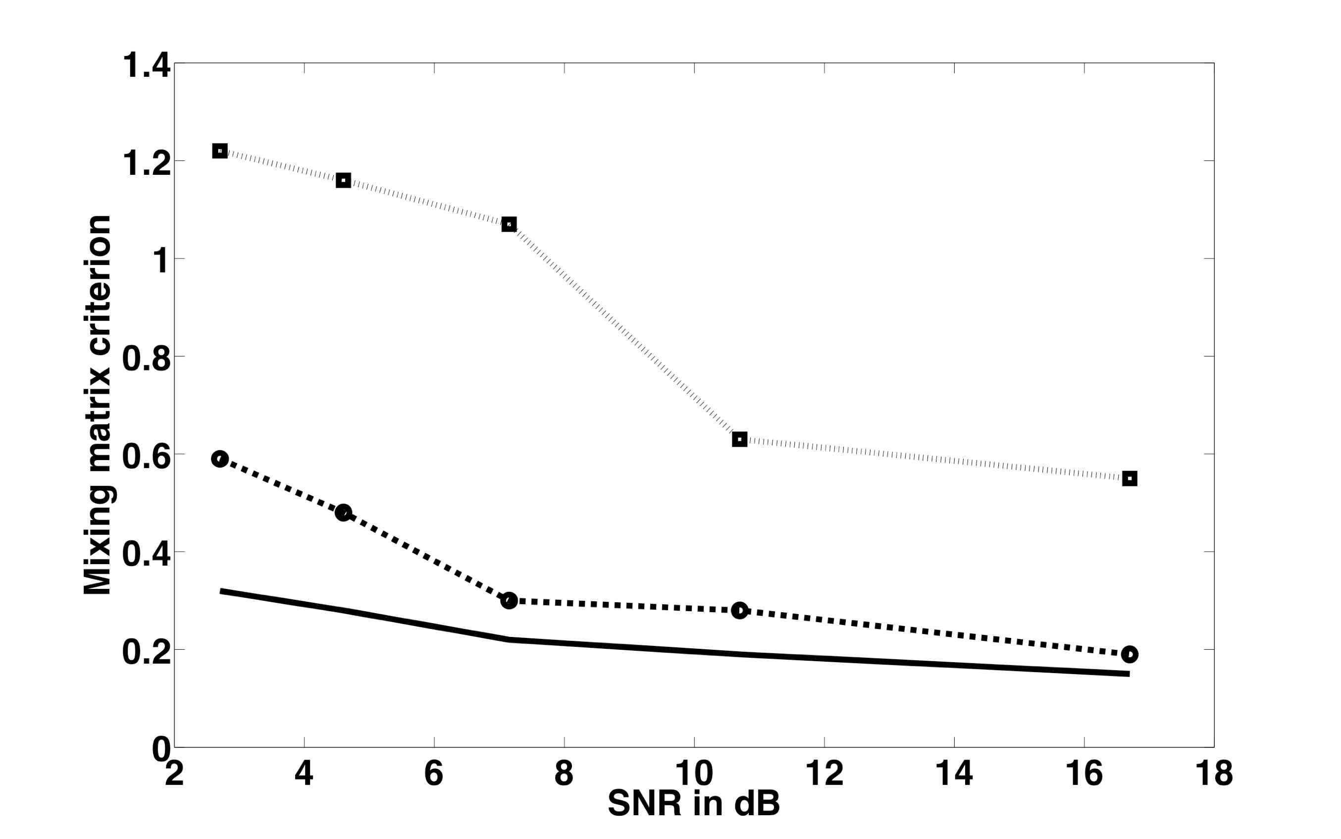
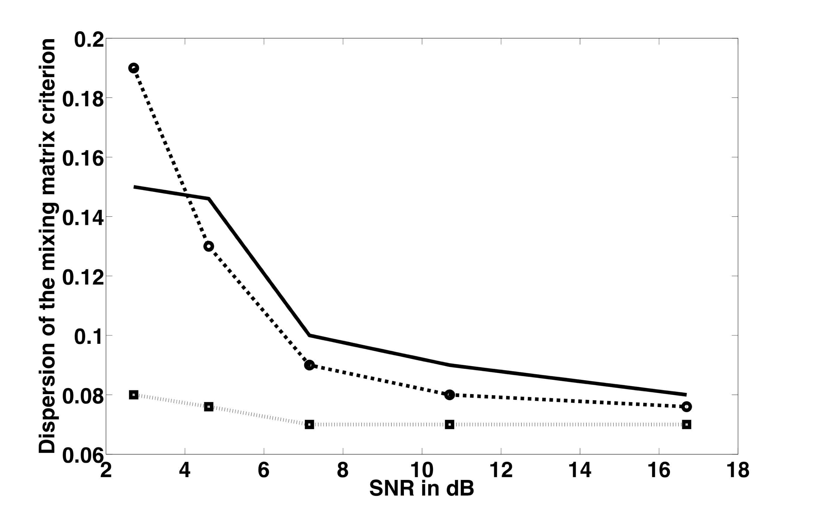
Figure 3 upper left panel shows the correlation coefficient between the true simulated CMB map and the one estimated by JADE (dotted line with $\Box$), SMICA (dashed line with $\circ$) and GMCA (solid line). The CMB map is well estimated by SMICA, which indeed was designed for the blind separation of stationary colored Gaussian processes, but not as well using JADE as one might have expected. GMCA turns out to perform similarly to SMICA. In the second line on the left of Figure 3, galactic dust is well estimated by both GMCA and SMICA. The SMICA estimates seem to have a slightly higher variance than GMCA estimates for higher global noise levels (SNR lower than $5$ dB). Finally, the picture in the third line on the left shows that GMCA gives better estimates of the SZ map than SMICA when the noise variance increases. The right panels provide the dispersion (i.e. standard deviation) of the correlation coefficients of the sources estimates. It appears that GMCA is a general method yielding simultaneous SZ and CMB estimates comparable to state-of-the-art blind separation techniques which seem mostly dedicated to individual components.
In a noisy context, assessing separation techniques turns out to be more accurate using a mixing matrix criterion. We define the mixing matrix criterion $\Delta_{\bf A}=\|{\bf I}-{\bf P}{\bf\hat{A}}^{-1}{\bf A}\|_{1,1}$ (where ${\bf P}$ is a matrix that reduces the scale/permutation indeterminacy of the mixing model, and $\|.\|_{1,1}$ is the entrywise $\ell_{1}$ matrix norm). Indeed, when ${\bf A}$ is perfectly estimated, it is equal to $\bf\hat{A}$ up to scale and permutation. As we entirely manage our experiments, the true sources and mixing matrix are known and thus ${\bf P}$ can be computed easily. The mixing matrix criterion is thus strictly positive unless the mixing matrix is perfectly estimated up to scale and permutation. This mixing matrix criterion is experimentally much more sensitive to separation error. The bottom right panel of Figure 3 illustrates the behavior of the mixing matrix criterion $\Delta_{\bf A}$ with JADE, SMICA and GMCA as the global noise variance varies. GMCA clearly outperforms SMICA and JADE when applied to CMB data.

2.2 Adding some physical constraint : the versatility of GMCA

In practice, the separation task is only partly blind. Indeed, the CMB emission law is extremely well-known. In this section, we illustrate that GMCA is versatile enough to account for such prior knowledge. In the following experiment, CMB-GMCA has been designed by constraining the column of the mixing matrix ${\bf A}$ related to CMB to its true value. This is equivalent to placing a strict prior on the CMB column of ${\bf A}$; that is $P(a^{cmb})=\delta(a^{cmb}-a^{cmb}_{0})$ where $\delta(.)$ is the Dirac measure and $a^{cmb}_{0}$ is the true simulated CMB emission law in the frequency range of Planck-HFI. Figure 4 shows the correlation coefficients between the true source maps and the source maps estimated using GMCA with and without the CMB prior.

Figure 4: Left Column : Mean value of the correlation coefficients between the estimated source map and the true source map - Right Column : Dispersion of these correlation coefficients : First line : CMB. Second line: galactic dust. Third line: SZ map. Legend : GMCA assuming that the CMB emission law is known : dotted line - GMCA : solid line. Abscissa : SNR in dB.

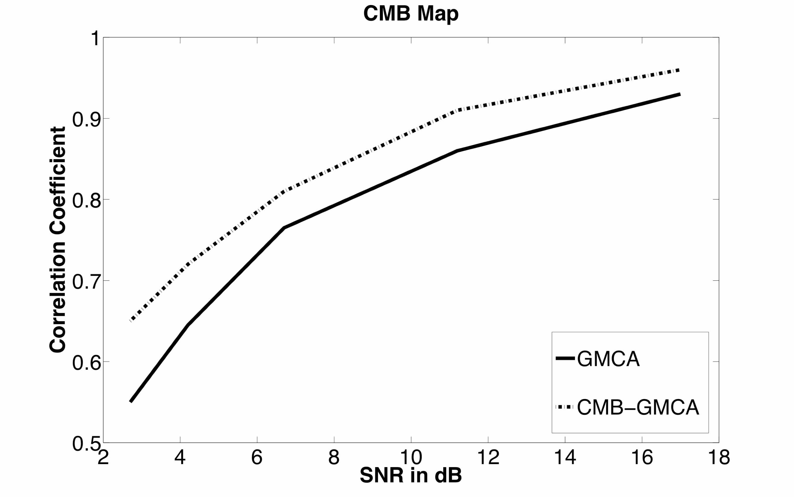
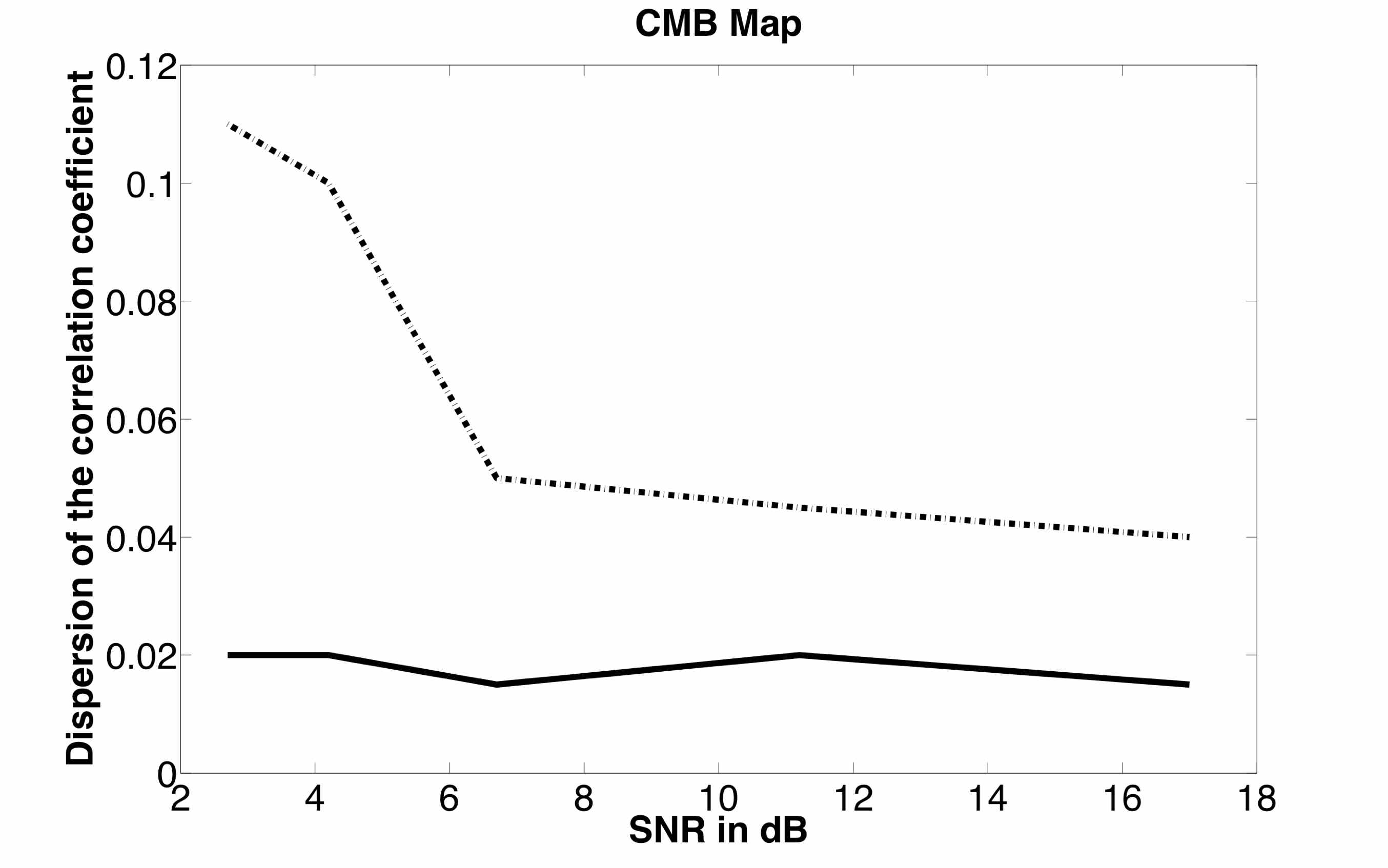
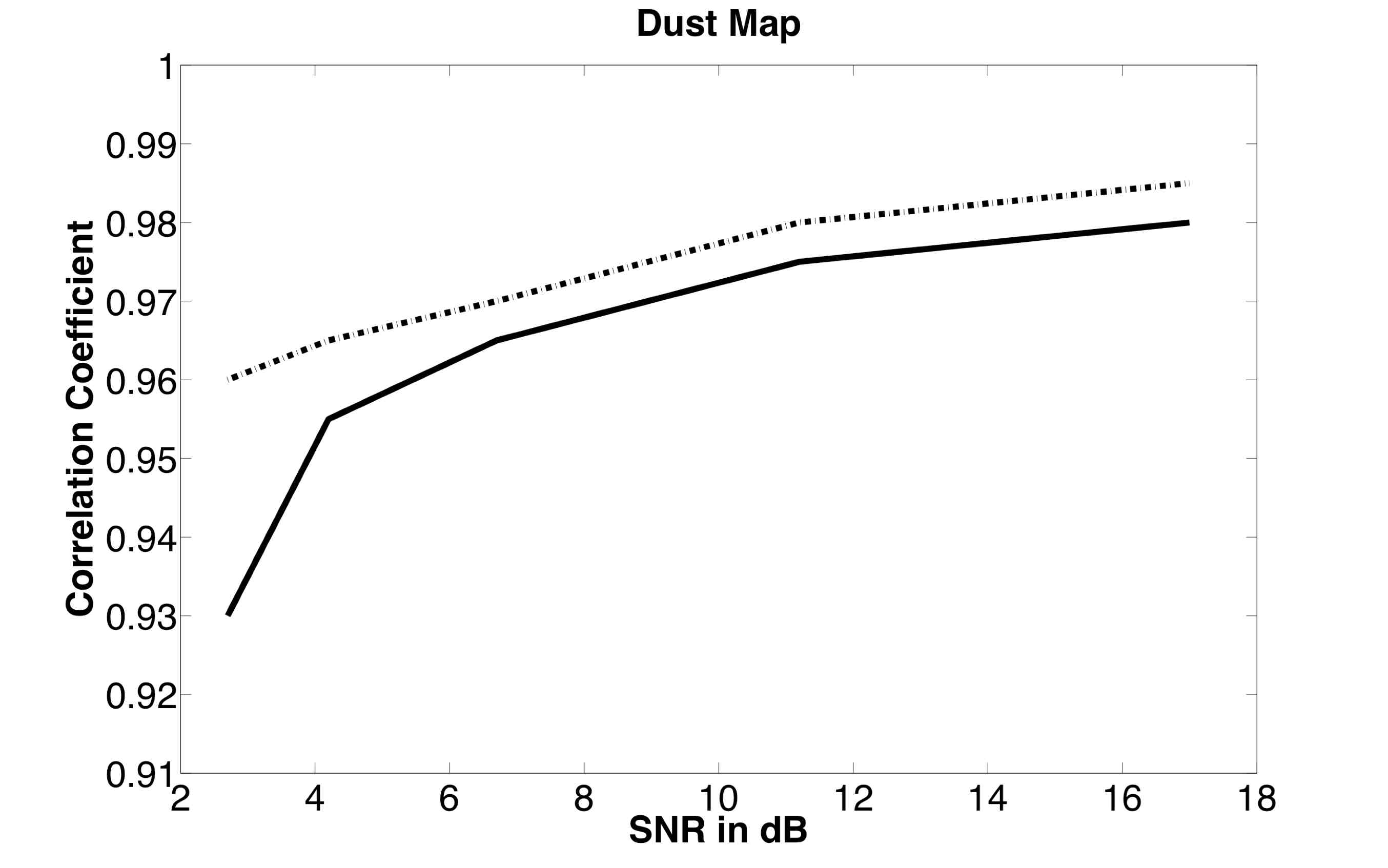
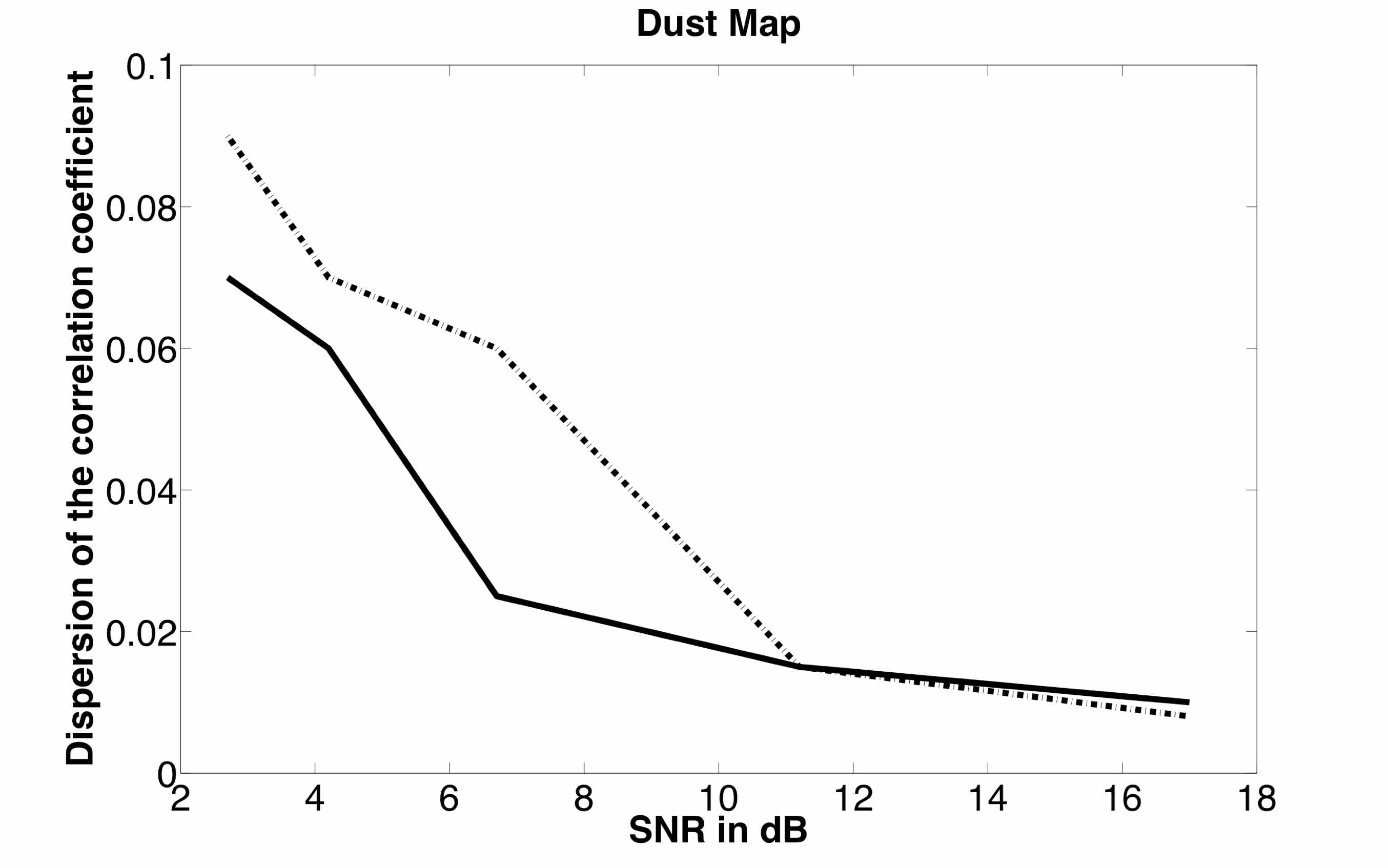
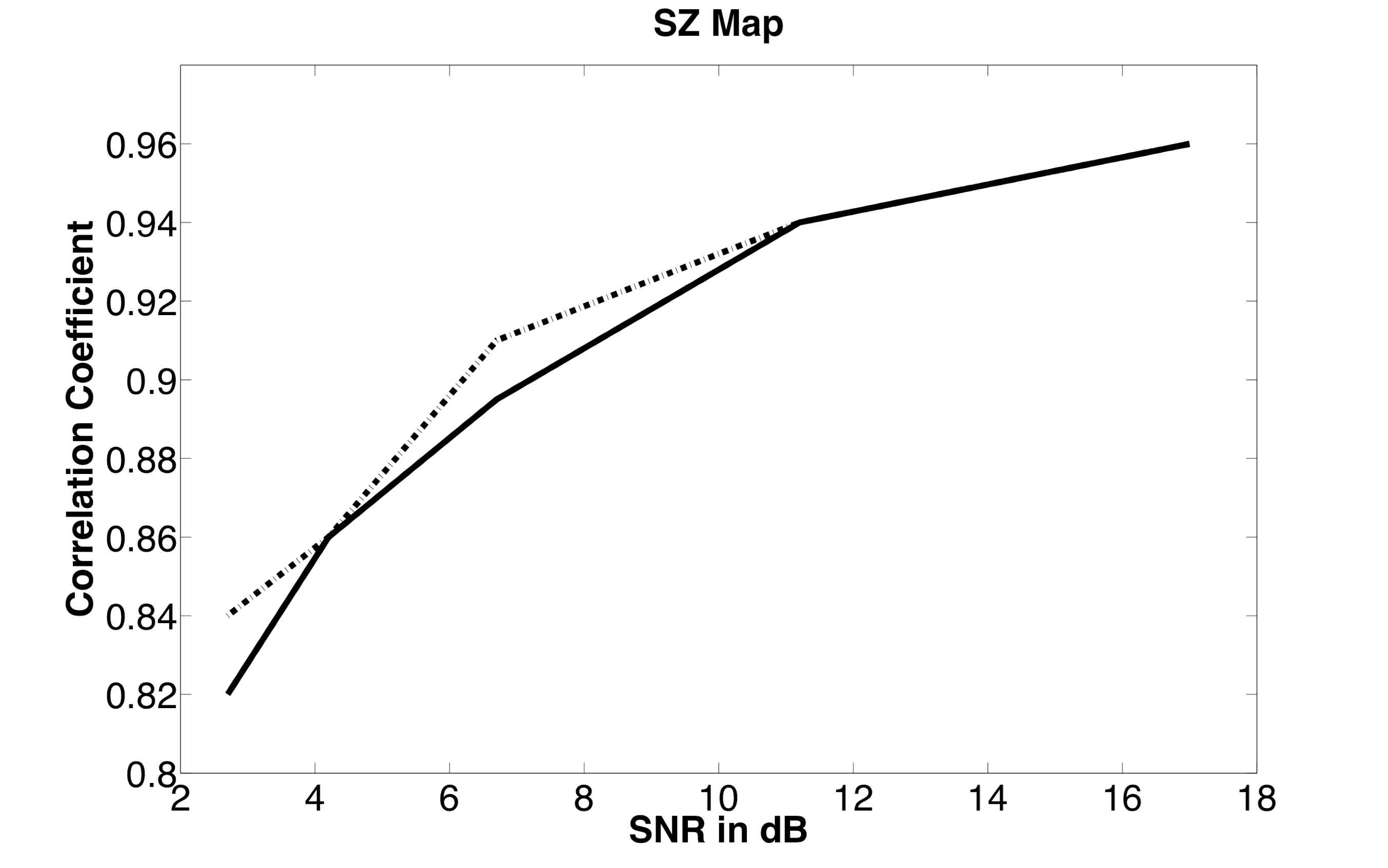
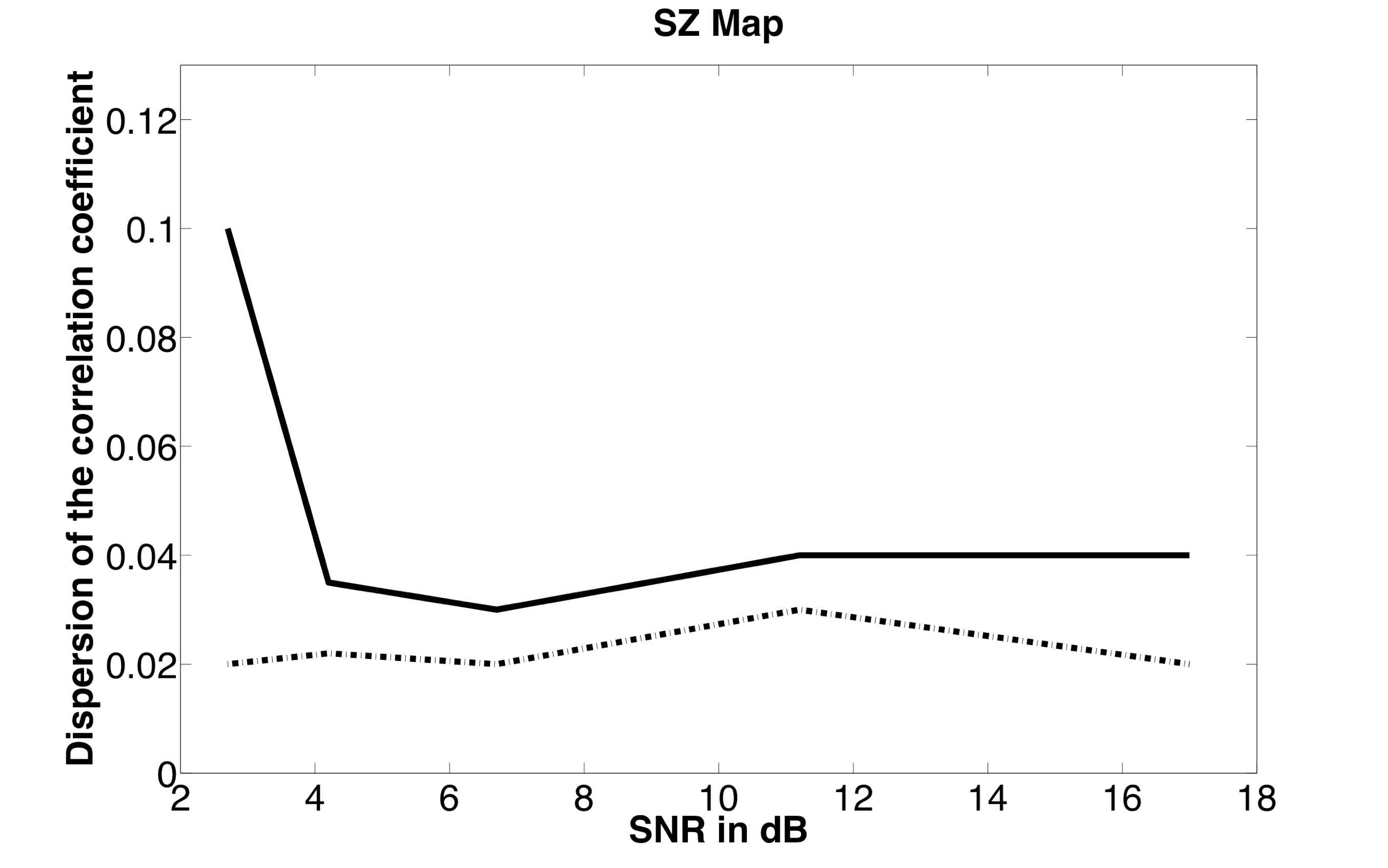
As expected, the top left picture of Figure 4 shows that assuming $a^{cmb}_{0}$ is known improves the estimation of CMB. Interestingly, the galactic dust map (in the middle on the left of Figure 4) is also better estimated. Furthermore, the CMB-GMCA SZ map estimate is likely to have a lower variance (bottom-right panel of Figure 4). Moreover, it is likely to provide more robustness to the SZ and galactic dust estimates thus enhancing the global separation performances.

3 Conclusion

In this paper we underlined that recovering information from CMB data requires solving a blind source separation issue (BSS). Several BSS techniques have already been applied to CMB data without providing good global performances i.e. on all components simultaneously. In this paper, we provide a sparsity-based source separation method coined Generalized Morphological Component Analysis (GMCA) which turns to give astounding results to effectively recover both CMB and SZ maps. In that context, sparsity enhances the contrast between the sources leading to an improved separation task even in a noisy context. In the blind case, when no prior knowledge is assumed on the emission laws of the components, GMCA outperforms state-of-the-art blind component separation techniques already applied to CMB data. Furthermore, GMCA is versatile enough to easily include some prior knowledge of the emission laws of the components. This is an extremely valuable feature of the proposed method in the case of CMB data analysis. Indeed, the CMB has a known black-body spectrum. Including this information in the GMCA algorithm enhances the source separation globally. In the present work, we have chosen not to include prior knowledge on the SZ spectral signature. Adding such prior would lead to even better separation results. Future work will be devoted to taking advantage of GMCA’s versatility to adapt to more complex physical models.

References

- [1] C.L.Bennett et al., “First year Wilkinson microwave anisotropy probe (WMAP) observations : preliminary maps and basic results”, ApJ. Suppl., vol. 148, 1, 2003.
- [2] J. Bobin, Y. Moudden, J.-L. Starck and M. Elad, “Morphological Diversity and Source Separation”, IEEE Signal Processing Letters, Vol.13, . 7, p. 409-412, July 2006.
- [3] R.Bouchet,R.Gispert,“Foregrounds and CMB Experiments: I. Semi-analytical estimates of contamination”, new astron. 4 443 (1999)
- [4] J.F. Cardoso, “The three easy routes to independent component analysis: contrast and geometry”, Proc. of ICA 2001 Workshop, San Diego, 2001.
- [5] J. Delabrouille, J.-F. Cardoso and G. Patanchon, “Multi-Detector Multi–Component spectral matching and applications for CMB data analysis”, Monthly Notices of the Royal Astronomical Society, 346, 4, 1089-1102, 2003.
- [6] D. L. Donoho and X. Huo, “Uncertainty principles and ideal atomic decomposition”, IEEE Transactions on Information Theory, vol. 47, no. 7, pp. 2845-2862, November, 2001.
- [7] O. Forni, N. Aghanim, 2004, Astron. Astrophys., 420, 49
- [8] G.Jungman et al., “Cosmological parameter determination with microwave backgroung maps”, Phys. Rev. D, 54, pp 1332-1344, 1996.
- [9] Y. Moudden, J.-F. Cardoso, J.-L. Starck, J. Delabrouille, “Blind Component Separation in Wavelet Space: Application to CMB Analysis”, Eurasip Journal on Applied Signal Processing , 2005, 15 pp 2437-2454, 2005.
- [10] S. Pires, J.-B. Juin, D. Yvon, Y. Moudden, S. Anthoine and E. Pierpaoli, “Sunyaev-Zeldovich cluster reconstruction in multiband bolometer camera surveys”, Astronomy and Astrophysics, 455 2 (2006) 741-755.
- [11] J.-L. Starck, M. Elad, and D.L. Donoho, “Image Decomposition Via the Combination of Sparse Representation and a Variational Approach”, IEEE Transaction on Image Processing , 14, 10, pp 1570–1582, 2005.
- [12] Sunyaev, R.A., & Zel’dovich, Ya.B., 1980, Ann. Rev. Astron. Astrophys., 18, 537
- [13] Tseng, P. (2001). “Convergence of a block coordinate descent method for nondifferentiable minimizations”, J. of Optim. Theory and Appl. 109, 3, pp. 457–494.
- [14] Zibulevsky, M. and Pearlmutter, B.A. (1999). “Blind Source Separation by Sparse Decomposition”, Neural Computations 13(4), 2001