A dispersive approach to pion photo- and electroproduction

Abstract

The relativistic amplitudes of pion photo- and electroproduction are calculated by dispersion relations at constant $t$. Several sum rules and low-energy theorems for the threshold amplitudes are investigated within this technique. The continuation of the amplitudes to sub-threshold kinematics is shown to provide a unique framework to derive the low-energy constants of chiral perturbation theory by global properties of the excitation spectrum.

1 Introduction

In two recent publications we have studied pion photoproduction on the nucleon in the framework of fixed-$t$ dispersion relations [1, 2]. In particular, we have concentrated on the threshold region in which the results can be compared to both precision data and predictions of baryon chiral perturbation theory (ChPT). The dispersion relations (DRs) are based on a set of 4 photoproduction amplitudes $A_{i}(\nu,t)$ depending on energy and momentum transfer described by the Lorentz invariant variables $\nu$ and $t$, respectively. These relations are Lorentz and gauge invariant by construction, and unitarity is implemented by constructing the real parts of the amplitudes from the imaginary (absorptive) parts via the dispersion integrals. The dispersive amplitudes for sub-threshold kinematics are regular functions in a region of small $\nu$ and $t$ values, and therefore they can be expanded in a power series about the origin of the Mandelstam plane ($\nu=0,\,t=0$). Comparing this series with the tree and loop contributions of relativistic baryon ChPT [3, 4, 5] one can read off the required low-energy constants (LECs) of that field theory, which up to now have been fixed by resonance saturation models or fits to the threshold data. In our present work we use MAID05 [6] as input for the absorptive parts of the amplitudes, which are obtained over the full resonance region up to c.m. energies of W=2.2 GeV by a global fit to the pion photoproduction data. With few exceptions the results compare favorably with the experimental data and the predictions of ChPT in the threshold region.

Another interesting aspect is the comparison with sum rules and low-energy theorems (LETs) of the 1950’s and 1960’s. These relations were based on current algebra and the PCAC hypothesis (partial conservation of the axial current). They become exact in the chiral limit of QCD, and thus all variables and observables have to be understood in the fictitious limit of vanishing (light) quark masses and hence soft pions with mass $M_{\pi}\rightarrow 0$. This leads to an expansion of the amplitudes in the mass ratio $\mu=M_{\pi}/M_{N}$. The first such theorem was established by Kroll and Ruderman [7] for charged pion photoproduction, with the result that the S-wave amplitude for this process was finite in the limit $\mu\rightarrow 0$, i.e., ${\mathcal{O}}(1)$. Somewhat later, several authors derived a LET for neutral pion photoproduction [8, 9], which led to the assumption that this reaction was ${\mathcal{O}}(\mu)$ for the proton and ${\mathcal{O}}(\mu^{2})$ for the neutron. However, extensive investigations in ChPT have shown that the finite pion mass leads to substantial corrections at physical threshold [10, 11]. We have studied the role of such corrections in the context of two sum rules of Fubini, Furlan, and Rossetti (FFR) [12]. The first of these sum rules relates the nucleon’s anomalous magnetic moment $\kappa_{N}$ to a dispersion integral over the first pion photoproduction amplitude $A_{1}(\nu,t)$ for neutral pions, or, if extended to electroproduction, the Pauli form factor to the corresponding electroproduction amplitude. The second FFR sum rule predicts that the difference of the axial ($G_{A}^{V}$) and the Dirac vector ($F_{1}^{V}$) form factors is related to the longitudinal electroproduction amplitude $A_{6}$ for charged pions. The radii of these form factors are of similar size, $\langle r^{2}\rangle_{1}^{V}-\langle r^{2}\rangle_{A}^{V}=(0.14\pm 0.03)$ fm${}^{2}\,$ and the early estimates [13] simply led to the result $G_{A}^{V}(Q^{2})-F_{1}^{V}(Q^{2})=0$. The first and to our knowledge only dispersive calculation was performed by Adler and Gilman already in 1966 [14]. Their result was $\langle r^{2}\rangle_{1}^{V}-\langle r^{2}\rangle_{A}^{V}=0.152$ fm², in fantastic agreement with our present knowledge of this observable. Unfortunately, this result involves a dispersion integral with formidable cancelations (I) among contributions of positive sign in the region up to the $\Delta(1232)$ resonance and of negative sign in the second resonance region and (II) between the electric transverse and longitudinal contributions of the same multipolarity.

We proceed by reviewing the status of the LET for neutral pion photoproduction in Sec. 2. The formalism for pion electroproduction is briefly described in Sec. 3. In the following Sec. 4 we discuss the FFR sum rule for the anomalous magnetic moment and compare the results of our dispersive calculation with the predictions of ChPT. We present some preliminary results on the two FFR sum rules for electroproduction in Sec. 5, and close by a short summary in Sec. 6.

2 Revised LET for neutral pion photoproduction

The “LET” of Refs. [8, 9] for the reaction $\gamma+p\rightarrow\pi^{0}+p$ was based on current algebra and PCAC. According to the theorem, the leading terms of the threshold multipole were to be given by the Born diagrams, evaluated with the pseudovector pion-nucleon interaction. However, this prediction had to be revised in the light of surprising experimental evidence. The reason for the discrepancy between the theorem and the data was first explained in the framework of ChPT by pion-loop corrections. An expansion of the S-wave amplitude in the mass ratio $\mu$ yielded the result [10, 11]

$$E_{0+}(\pi^{0}p)=\frac{eg_{\pi N}}{8\pi m_{\pi}}\left\{\mu-\mu^{2}\,\frac{3+\kappa_{p}}{2}-\mu^{2}\,\frac{M^{2}}{16f^{2}_{\pi}}+\ ...\right\}\ ,$$ (1)

where $g_{\pi N}$ is the pion-nucleon coupling constant and $f_{\pi}\approx 93$ MeV the pion decay constant. The first and the second terms on the rhs of Eq. (1) are the prediction of Refs. [8, 9], which however has to be corrected by the third term on the rhs. Although this loop correction is formally of higher order in $\mu$, its numerical value is of the same size as the leading term.

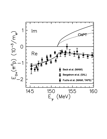
Figure 1: The real (Re) and imaginary (Im) parts of the S-wave amplitude $E_{0+}$ for $\pi^{0}$ photoproduction at threshold energies. The MAMI data [15, 16] are represented by circles, the SAL data [17] by triangles. Dashed lines: predictions of ChPT at $\cal{O}$($p^{3}$) [18, 19], solid lines: results from dispersion relations [20]. The solid horizontal line at about -2.2 shows the prediction of Refs. [8, 9].

The energy dependence of $E_{0+}(\pi^{0}p)$ is shown in Fig. 1. The discrepancy between the prediction of Refs. [8, 9] and the experimental data obtained at the Mainz Microtron MAMI and at SAL (Saskatoon) is apparent. Furthermore, the real part of the amplitude shows a characteristic “Wigner cusp” at the threshold for charged pion production, which lies about 5 MeV above the $\pi^{0}$ threshold. This cusp in the real part is related to the sharp rise of the imaginary part at the second threshold. The physical picture behind the large loop correction is based on (I) the large production rate of the charged pions and (II) the charge-exchange scattering between the nucleon and the slow $\pi^{+}$ in the intermediate state, which leaves a $\pi^{0}$ in the final state. However, the direct experimental determination of the imaginary part will require double-polarization experiments with linearly polarized photons and polarized targets. The excellent agreement between ChPT and the data for $E_{0+}$ is somewhat flawed by the fact that higher order diagrams are sizeable, that is, the perturbative series converges slowly and low-energy constants appearing at the higher orders reduce the predictive power.

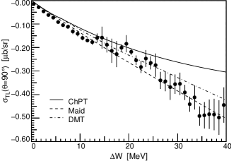
Figure 2: The separated cross sections $\sigma_{0}$, $\sigma_{\rm{TL}}$, and $\sigma_{\rm{TT}}$ as well as the beam helicity asymmetry $A_{\rm{TL}}^{\prime}$, as function of $\Delta W=W-W_{\rm{thr}}$ and at the pion c.m. angle $\theta_{\pi}=90^{\circ}$. Solid line: HBChPT [24], dashed line: MAID [6], and dashed-dotted line: DMT model [25]. The data are from Weis et al. [23].

The great success of ChPT for photoproduction at threshold was a strong motivation to extend the experimental program to electroproduction. The first of such investigations were performed at NIKHEF [21] and MAMI [22] for $Q^{2}=0.10~{}$GeV², and provided another confirmation of ChPT although at the expense of 2 new low-energy constants, which were fitted to the data. In order to further check this agreement, data were also taken at lower momentum transfer. Whereas the former experiments were only sensitive to the real part of the amplitudes, Weis et al. [23] also determined the fifth structure function (${\rm{TL}}^{\prime}$), which contains information on the phase of the S-wave amplitude. The result is displayed in Fig. 2. We observe that only the dynamical Dubna-Mainz-Taipei (DMT) model [25] is able to fully describe the experiment, in particular its prediction for the helicity asymmetry is right on top of the data. Such dynamical models start from a description of the pion-nucleon scattering phases by a quasi-potential, which serves as input for an integral equation to account for multiple scattering. In this sense the model contains the loop corrections to an arbitrary number of rescattering processes, and is therefore perfectly unitary, albeit on a phenomenological basis that may violate gauge invariance to some extent.

3 Formalism

Let us consider the reaction $\gamma^{\ast}(q)+N(p)\rightarrow\pi(k)+N(p\,^{\prime})$, where the variables in brackets denote the four-momenta of the participating particles. The familiar Mandelstam variables are $s=(p+k)^{2},\,t=(q-k)^{2}$, and $u=(p-q)^{2}$, and $\nu=(s-u)/(4M_{N})$ is the crossing-symmetric variable. The latter variable is related to the photon lab energy $E_{\gamma}^{\rm{lab}}$ by $\nu=E_{\gamma}^{\rm{lab}}+(t-M_{\pi}^{2}+Q^{2})/(4M_{N})$. The physical $s$-channel region is shown in Fig. 3. Its upper and lower boundaries are given by the scattering angles $\theta=0$ and $\theta=180^{\circ}$, respectively. The nucleon and pion poles lie in the unphysical region and are indicated by the dotted lines at $\nu_{s}=\nu_{B}$ ($s$-channel) and $\nu_{u}=-\nu_{B}$ ($u$-channel), where $\nu_{B}=(t-M_{\pi}^{2}+Q^{2})/(4M_{N})$, and $t=M_{\pi}^{2}$ ($t$-channel).

Figure 3: The Mandelstam plane for pion photoproduction ($Q^{2}=0$) on the nucleon. The boundaries of the physical region are $\theta=0$ (forward production) and $\theta=180^{\circ}$ (backward production). The nucleon and pion pole positions are indicated by the dotted lines $s=M_{N}^{2}$, $u=M_{N}^{2}$, and $t=M_{\pi}^{2}$. The dashed line $s=(M_{N}+M_{\pi})^{2}$ indicates the threshold of pion production and therefore also of the imaginary part of the production amplitude. It is tangent to the boundary of the physical region in the point $\nu=\nu_{\rm{thr}}$, $t=t_{\rm{thr}}$. The path $t=t_{\rm{thr}}$ (dashed-dotted line) yields the only dispersion relation at $t={\rm{const}}$ whose imaginary part is fully contained in the physical region.

The nucleonic transition current can be expressed in terms of 6 invariant amplitudes $A_{i}$, $J^{\mu}=\sum_{i=1}^{6}A_{i}(\nu,t,Q^{2})\,M^{\mu}_{i}$, with the four-vectors $M^{\mu}_{i}$ given by the independent axial vectors constructed from the particle momenta and the Dirac $\gamma$ matrices [26]. In the case of real photons ($Q^{2}=0$) and with the gauge condition $\epsilon_{\mu}k^{\mu}=0$, the matrices $M^{\mu}_{5}$ and $M^{\mu}_{6}$ do not contribute to the interaction Lagrangian, and the remaining 4 matrices reduce to Eq. (10) of Ref. [1]. The invariant amplitudes $A_{i}$ can be further decomposed into three isospin channels ($a=1,2,3$), $A_{i}^{a}=A_{i}^{(-)}i\epsilon^{a3b}\tau^{b}+A_{i}^{(0)}\tau^{a}+A_{i}^{(+)}\delta_{a3}$, where $\tau^{a}$ are the Pauli matrices in isospace, and the physical photoproduction amplitudes are given by

$$A_{i}(\gamma p\rightarrow n\pi^{+})=+\sqrt{2}(A_{i}^{(-)}+A_{i}^{(0)}), A_{i}(\gamma p\rightarrow p\pi^{0})=A_{i}^{(+)}+A_{i}^{(0)},$$

$$A_{i}(\gamma n\rightarrow p\pi^{-})=-\sqrt{2}(A_{i}^{(-)}-A_{i}^{(0)}), A_{i}(\gamma n\rightarrow n\pi^{0})=A_{i}^{(+)}-A_{i}^{(0)}.$$ (2)

Under crossing, the amplitudes $A_{1,2,4}^{(+,0)}$ and $A_{3,5,6}^{(-)}$ are even functions of $\nu$ and satisfy a DR of the type

$${\rm Re}\,A^{I}_{i}(\nu,t,Q^{2})=A_{i,{\rm pole}}^{I}(\nu,t,Q^{2})+\frac{2}{\pi}{\cal P}\int_{\nu_{\rm{thr}}}^{\infty}{\rm d}\nu^{\prime}\,\frac{\nu^{\prime}\,{\rm Im}\,A_{i}^{I}(\nu^{\prime},t,Q^{2})}{\nu^{\prime 2}-\nu^{2}}\,,$$ (3)

whereas the amplitudes $A_{3,5,6}^{(+,0)}$ and $A_{1,2,4}^{(-)}$ are odd and therefore fulfil the relation

$${\rm Re}\,A^{I}_{i}(\nu,t,Q^{2})=A_{i,{\rm pole}}^{I}(\nu,t,Q^{2})+\frac{2\nu}{\pi}{\cal P}\int_{\nu_{\rm{thr}}}^{\infty}{\rm d}\nu^{\prime}\,\frac{{\rm Im}\,A_{i}^{I}(\nu^{\prime},t,Q^{2})}{\nu^{\prime 2}-\nu^{2}}\,.$$ (4)

We note that these amplitudes have no kinematic but only dynamic singularities (poles and cuts). As a consequence, the integrals on the rhs of Eqs. (3) and (4) yield real and regular functions in a triangle bounded by the onset of particle production, that is below the cuts from $\pi\pi$ states at $t\geq 4M_{\pi}^{2}$ and N$\pi$ states for $s,u\geq(M_{N}+M_{\pi})^{2}$. Therefore, the integrals (“dispersive contributions”) can be expanded in a Taylor series about the origin of the Mandelstam plane. In order to avoid the cluttering of indices in the following text, we denote the real part of the dispersive amplitudes simply by ${\rm Re}A^{I}_{i,{\rm disp}}={\rm Re}A^{I}_{i}-A^{I}_{i,{\rm pole}}\doteq A_{i}^{I}$.

4 Anomalous magnetic moment

The FFR prediction for the Pauli form factor can be cast in the following form:

$$F_{2}^{N}(Q^{2})\tau_{3}+\Delta_{N}(\nu,t_{\rm{thr}},Q^{2})=\frac{4M_{N}^{2}}{\pi eg_{\pi N}}{\cal P}\int_{\nu_{\rm{thr}}}^{\infty}{\rm d}\nu^{\prime}\,\frac{\nu^{\prime}\,{\rm Im}\,A_{1}^{(N,\pi^{0})}(\nu^{\prime},t_{\rm{thr}},Q^{2})}{\nu^{\prime 2}-\nu^{2}}\,,$$ (5)

where $\Delta^{N}(\nu,t,Q^{2})$ is the “FFR discrepancy”, which should vanish in the soft-pion limit, $\nu\rightarrow 0,\nu_{B}\rightarrow 0,M_{\pi}\rightarrow 0$. In this limit, the pion threshold moves to the point ($\nu=0$, $t=-Q^{2}$) of the Mandelstam plane, which lies in the unphysical region. In the following we concentrate on the question whether the anomalous magnetic moment $\kappa_{N}=F_{2}^{N}(0)$ can be determined from the photoproduction data. The integrand for the dispersion integral of Eq. (5) is plotted in Fig. 4 for real photons ($Q^{2}=0$) and at $\nu=0$ (dashed lines) as well as $\nu=\nu_{\rm{thr}}$ (solid lines). In accordance with the magnetic moments, the isoscalar combination (top) is small compared to the isovector one (bottom).

Figure 4: The integrands of the dispersion integrals on the rhs of Eq. (5) for the isoscalar (top) and isovector (bottom) combinations of the amplitudes $A_{1}(\nu,t_{\rm{thr}},0)$. The full lines are obtained for $\nu=\nu_{\rm{thr}}$, the dashed lines for $\nu=0$.

The isoscalar integrand (top) shows peaks at threshold (S-wave pion production), no contribution in the $\Delta(1232)$ region, and further peaks in the second and third resonance regions. The isovector integrand (bottom) is essentially given by S-wave threshold production and a large contribution of the $\Delta(1232)$, whereas the higher resonance regions are negligible. However we note that the size of the S-wave contribution decreases strongly if the integral is evaluated in sub-threshold kinematics, for example, at $\nu=0$ as shown by the dashed lines in the figure.
In Fig. 5 we investigate the convergence of the multipole expansion for the dispersion integral of the proton. The figure shows the lhs of Eq. (5) evaluated over a large energy range. The result is clearly dominated by the imaginary part of the P-wave amplitude (dotted line), but the S-wave contribution is substantial at low $\nu$ values and yields the cusp effect at threshold (dashed line). The imaginary parts of the higher partial waves turn out to be negligible over the whole energy region.

Figure 5: The values of $\kappa_{p}+\Delta_{p}(\nu,t_{\rm{thr}})$ obtained from the dispersion integral of Eq. (5) with a multipole decomposition of Im$A_{1}$. Solid line: full result for Im$A_{1}$ evaluated with MAID03. Dashed line: result for the dispersion integral with only the S-wave contribution to Im$A_{1}$, dotted line: P-wave contribution only, dashed-dotted line: sum of D- and F-wave contributions.

We observe that the FFR theorem is nearly fulfilled in the sub-threshold region, for $\nu\rightarrow 0$. Indeed, the result of the dispersion integral is very close to $\kappa_{p}=1.793$, and by increasing $t$ from $t_{\rm{thr}}$ to $M_{\pi}^{2}$, the FFR discrepancy decreases even further. In this sense we may conclude that the proton’s anomalous magnetic moment is produced to $\frac{1}{3}$ by S-wave pions near threshold and $\frac{2}{3}$ by P waves, mostly from $\Delta(1232)$ resonance excitation. The following Fig. 6 compares the predictions of Heavy Baryon (HB) ChPT and DR for $\Delta_{p}(\nu,t_{\rm{thr}},0)$ as function of $\nu$ in the range $0\leq\nu\leq 200$ MeV. Although there is good agreement in the threshold region (upper panel), we observe 3 principal differences between HBChPT and DR if we move further away from the threshold (lower panel): (I) The rise of $\Delta_{p}$ for $\nu\gtrsim 170$ MeV due to the $\Delta(1232)$ resonance cannot be described by the “static” LECs of HBChPT, but requires a dynamical description of the resonance degrees of freedom  [28, 29]. (II) The curvature predicted by HBChPT for small $\nu$ is due to the non-relativistic approach, which leads to shifts of the nucleon pole situated at $\nu=\nu_{B}=-9.7$ MeV and, along the same line, to violations of the crossing symmetry. (III) Different order approximations of HBChPT lead to quite different results in the sub-threshold region.

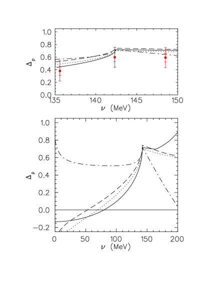
Figure 6: The correction to the FFR sum rule for the proton, $\Delta_{p}(\nu,t_{\rm{thr}},0)$ as defined by Eq. (5). The dispersive approach (solid lines) is compared to several predictions of HBChPT, represented by the dotted [18], dashed [19], and dashed-dotted [27] lines. The data points are obtained from the experimental S- and P-wave multipoles of Ref. [33] and an estimate of the D waves according to MAID.

The shortcomings of HBChPT have of course been noted often before, and several groups are now applying newly developed manifestly Lorentz-invariant renormalization schemes [30, 31, 32] to various physical processes, in particular also to pion photoproduction. However, the general structure of the dispersive part of the (dispersive) amplitude $A_{1}$ for small external momenta has already been given in Ref. [3],

$$A_{1}^{(N,\pi^{0})}=a_{00}+a_{02}\nu_{B}(t)+a_{20}\nu^{2}+\ldots\,,$$ (6)

where the coefficients $a_{ik}$ are functions of the mass ratio $\mu$. In particular the leading coefficients depend on the pion mass as follows: $a_{00}={\mathcal{O}}\,(\mu^{2})$, $a_{02}={\mathcal{O}}\,(\ln\,\mu)$, and $a_{20}={\mathcal{O}}\,(\mu^{-1})$. The vanishing of $a_{00}$ in the chiral limit is, of course, a necessary condition for the validity of the FFR sum rule. Furthermore, the divergence of the higher expansion coefficients in that limit is the reason why the old LET for neutral pion photoproduction failed. The analytic continuation of the multipole expansion for $A_{1}$ to the soft-pion threshold at the unphysical point ($s=u=M_{N}^{2},t=M_{\pi}^{2}$) requires some care, because the Legendre polynomials $P_{\ell}(x)$ involved in the expansion have to be evaluated at $|x|>1$. As a result of this extrapolation we find that $\delta_{00}^{N}$ is zero within the error bars of our calculation, which are essentially due to the unknown higher part of the spectrum. Also the expansion in $\nu_{B}(t)$ requires an extrapolation to the unphysical region near the origin of the Mandelstam plane. However, the coefficients of $\nu^{2n}$, $n\geq 1$, can be (approximately) obtained by expanding the dispersion integral at $t=t_{\rm{thr}}$ in a power series in $\nu^{2}$,

$$a_{2n,0}^{N}\approx\frac{4M_{N}^{2}}{\pi eg_{\pi N}}\,\int_{\nu_{\rm{thr}}}^{\infty}\frac{d\nu^{\prime}}{(\nu^{\prime})^{2n+1}}\,{\rm Im}\,A_{1}^{(N,\pi^{0})}(\nu^{\prime},t_{\rm{thr}},0)\,.$$ (7)

Due to the additional factors of $1/\nu^{\prime}\,{}^{2}$, these integrals are well saturated by the region between threshold and the $\Delta(1232)$ resonance. The numerical results for these coefficients are $a_{20}^{p}=0.368/M^{2}_{\pi+}$, $a_{40}^{p}=0.120/M^{4}_{\pi+}$, and $a_{60}^{p}=0.054/M^{6}_{\pi+}$, and Fig. 7 shows the good convergence of the Taylor series below pion threshold.

Figure 7: Full line: the correction $\Delta_{p}(\nu,t_{\rm{thr}},0)$ as defined by Eq. (5), compared to the low-energy expansion in the crossing-symmetric variable $\nu$. Dashed line: expansion up to ${\mathcal{O}}(\nu^{2})$, dashed-dotted line: to ${\mathcal{O}}(\nu^{4})$, dotted line: to ${\mathcal{O}}(\nu^{6})$.

We note that these results are obtained by expanding the denominator $\nu^{\prime 2}-\nu^{2}$ in the dispersion integral for fixed $t_{\rm{thr}}$ and $Q^{2}=0$. This expansion converges up to the cusp at $\nu=\nu_{\rm{thr}}$. In the same way, also the loop terms of relativistic ChPT can be expanded in a real power series in $\nu^{2}$ about $\nu=0$, up to the singularity at threshold. The Born and counter terms are power series in $\nu^{2}$ anyway. It is therefore possible to determine the (unknown) low-energy constants by comparing the Taylor expansions of ChPT and DR in the sub-threshold region.

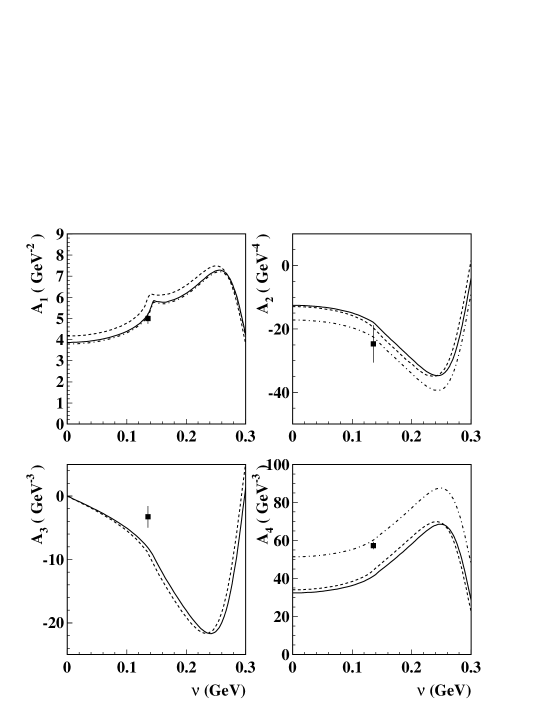
Figure 8: The real parts of the amplitudes $A_{i}^{(p\pi^{0})}$ for the reaction $\gamma p\to\pi^{0}p$ as function of $\nu$ and at $t=t_{\rm{thr}}$. Solid lines: dispersive contributions according to Eqs. (3) and (4) as evaluated with the imaginary amplitudes from MAID05 containing partial waves up to $\ell_{\rm{max}}=3$. Dashed lines: same results calculated with SAID [38]. The dashed-dotted lines are obtained by adding the vector-meson contributions to the MAID result. The data points near threshold are derived from the experimental values of Ref. [33] for the S and P waves plus the MAID values for the D waves.

Figure 8 displays the 4 invariant amplitudes for neutral pion photoproduction on the proton. The agreement between the MAID and SAID results demonstrates that the imaginary parts of the amplitudes, which serve as input for the dispersion integrals, are quite similar in these two partial-wave analyses. We further observe that the cusp effect is only dominant for the amplitude $A_{1}$, which signifies that the other 3 amplitudes have only small contributions from S waves and loop effects. However, the dispersion integrals can not fully describe the experimental values for $A_{2}$ to $A_{4}$. The reason is that these integrals do not provide the pole structures of the vector mesons at $t=m_{V}^{2}$, even though the vector meson background plays an important role in the unitarization process of MAID. It is even more surprising that the dispersion integrals for the threshold amplitudes change only by a few percent if we drop the vector mesons in the construction of the absorptive amplitude by MAID, whereas the vector mesons yield 20 % and 50 % of the threshold amplitudes for $A_{2}$ and $A_{4}$, respectively. We therefore have to accept the Mandelstam hypothesis [34] that the amplitudes are the sum of all pole terms plus two-dimensional integrals over the double spectral region. The one-dimensional DRs, e.g. at $t=$const, follow from this representation, as has been proved for pion photoproduction by Ball [35]. Alternatively, we could subtract the DRs at $\nu=0$, which introduces an unknown function $A_{i}^{I}(0,t,0)$. This function is real in the region of small $t$, and in principle can be constructed from its imaginary part by an integral along the $t$-axis of Fig. 3. If we add the t-channel $\rho$ and $\omega$ poles according to MAID05, we obtain an almost perfect agreement for $A_{1}$, $A_{2}$ and $A_{4}$. The apparent discrepancy between theory and experiment for $A_{3}$ is an open question. The inclusion of the vector meson poles does not help, because only axial vector mesons can contribute to the crossing-odd amplitude $A_{3}^{(p\pi^{0})}$ [2].
Let us next expand all 4 amplitudes for neutral pion photoproduction about the point ($\nu=0,\,t=M_{\pi}^{2},Q^{2}=0$). We first define dimensionless quantities $\Delta_{i}(\nu,t,0)$ as follows:

$$A_{1}(\nu,t,0) = \frac{eg_{\pi N}}{2M_{N}^{2}}\,(\kappa+\Delta_{1}(\nu,t,0))\,,$$

$$A_{2}(\nu,t,0) = \frac{eg_{\pi N}}{2M_{N}^{4}}\,\Delta_{2}(\nu,t,0)\,,$$ (8)

$$A_{3,4}(\nu,t,0) = \frac{eg_{\pi N}}{2M_{N}^{3}}\,\Delta_{3,4}(\nu,t,0)\,.$$

The functions $\Delta_{i}(\nu,t,0)$ are regular near the origin of the Mandelstam plane and can be expanded in a power series in $\nu$ and $t$ (or $\nu_{B}(t)$). As is evident from the definition of the variables, $\nu$ is ${\mathcal{O}}(M_{\pi})$ and $\nu_{B}$ is ${\mathcal{O}}(M_{\pi}^{2}/M_{N})$ in the region of interest. Therefore the crossing-even amplitudes $\Delta_{1,2,4}^{(+,0)}$ and $\Delta_{3}^{(-)}$ have the expansion

$$\Delta_{i}(\nu,t,0)=\delta_{00}^{i}+\delta_{20}^{i}\,\nu^{2}/M_{\pi}^{2}+\delta_{02}^{i}\,\nu_{B}/M_{\pi}+\ldots\,,$$ (9)

with the lowest expansion parameters given by

$$\delta_{00}^{i} = \Delta_{i}(0,\,M^{2}_{\pi},0)\,,$$

$$\delta_{20}^{i} = \frac{M_{\pi}^{2}}{2}\frac{\partial^{2}}{\partial\,\nu^{2}}\,\Delta_{i}(\nu\,,M^{2}_{\pi},0)\big{|}_{\nu=0}\,,$$

$$\delta_{02}^{i} = 4M_{N}\,M_{\pi}\frac{\partial}{\partial\,t}\,\Delta_{i}(0,t,0)\big{|}_{t=M^{2}_{\pi}}\,.$$ (10)

The expansion of the crossing-odd amplitudes $\Delta_{3}^{(+,0)}$ and $\Delta_{1,2,4}^{(-)}$ takes the form

$$\Delta_{i}(\nu,t,0)=\delta_{10}^{i}\,\nu/M_{\pi}+\delta_{30}^{i}\,\nu^{3}/M_{\pi}^{3}+\delta_{12}^{i}\,\nu\nu_{B}/M_{\pi}^{2}+\ldots\,,$$ (11)

with the lowest expansion parameter

$$\delta_{10}^{i}=M_{\pi}\frac{\partial}{\partial\nu}\,\Delta(\nu,M_{\pi}^{2})\big{|}_{\nu=0}\,.$$ (12)

Table 1: The leading expansion coefficients for the $p\pi^{0}$ amplitudes from the dispersion integral (see Eqs. (8)-(12) for definitions) including the vector meson $t$-channel contributions. In brackets: the low-energy constants of ChPT [5].

	$\delta_{00}$	$\delta_{10}$	$\delta_{20}$	$\delta_{02}$
$A_{1}$	-0.04  (0)	-	0.32  (0.53)	1.68  (3.40)
$A_{2}$	-6.41  (-6.33)	-	-1.26	1.92
$A_{3}$	-	-2.23 (-2.58)	-	-
$A_{4}$	21.19  (22.40)	-	2.23	4.50

In Table 1 we list the leading expansion coefficients for the full $p\pi^{0}$ amplitudes obtained from the dispersive calculation. The numbers in brackets are the LECs of relativistic ChPT. The differences between the full dispersive result and the LECs indicate the size of the loop terms and, in the case of $A_{1}$, also of the FFR current. It is obvious that the loop contributions are small for the amplitudes $A_{2}$, $A_{3}$, and $A_{4}$.

5 Pion electroproduction

The threshold for pion electroproduction moves with the value of $Q^{2}$, and in the following we evaluate the dispersive amplitude $t=t_{\rm{thr}}(Q^{2})$ along the path from $\nu=\nu_{\rm{thr}}(Q^{2})$ to infinity. In the soft-pion limit, the threshold moves to $\nu=0$ and $t=-Q^{2}$ (or $\nu_{B}=0$). As in the previous section for real photons, we can extrapolate from the physical to the soft-pion threshold for small values of $\nu$, $\nu_{B}$, and $Q^{2}$. Of course, we can not expect to reproduce the FFR sum rule in this way, because the expansion coefficients of the FFR discrepancy depend on the pion mass and the dispersion calculation only provides these coefficients for the physical mass. In particular the pion-loop effects at threshold depend on the pion mass and, moreover, they produce a $Q^{2}$ dependence very different from the nucleon form factors. However, as has been shown before, we expect a suppression of these loop effects if the dispersion integral is evaluated in the sub-threshold region.

Figure 9: The proton’s Pauli form factor $F_{2}^{p}$ as function of $Q^{2}$ compared to the rhs of Eq. (5). Thick solid line: dispersive results at threshold ($\nu=\nu_{\rm{thr}},t=t_{\rm{thr}}$), thick dashed line: same kinematics but including the $t$-channel vector meson poles, thin solid line: dispersive results for soft-pion kinematics ($\nu=\nu_{B}=0$), thin dashed line: same kinematics but including the $t$-channel vector meson poles. The dashed-dotted line is the parametrization of $F_{2}^{p}$ according to Ref. [37].

In Fig. 9 we compare the Pauli form factor $F_{2}^{p}$ (dotted line) to the $Q^{2}$ dependence of $A_{1,\,\rm{disp}}^{(p\pi^{0})}$ as evaluated by the dispersion integral at $\nu=0$ and $\nu=\nu_{\rm{thr}}$. The figure clearly demonstrates that the slopes of the Pauli form factor and the invariant amplitude $A_{1,\,\rm{disp}}^{(p\pi^{0})}$ differ considerably. More quantitatively, the extrapolation to the soft-pion kinematics yields an effective r.m.s. radius $r[A_{1}(\nu=\nu_{B}=0)]\approx 1.12$ fm, much larger than the Pauli radius of the proton, $r_{2}^{p}=0.894$ fm [36] or $0.879$ fm [37]. The reason for this behavior is already seen from the integrand of the dispersion integral shown in the top panels of Fig. 10 for the momentum transfers $Q^{2}=0$ and $0.1$ GeV². Evidently the bulk contribution to the integral stems from the $\Delta(1232)$ resonance. In the real photon limit and for energies near threshold (solid line) also the S-wave threshold production is quite sizeable, but this contribution of the pion cloud decreases rapidly if the energy moves into the sub-threshold region. It is also seen that the loop effects drop faster with momentum transfer than the resonance contributions. As discussed in the previous section, the FFR prediction is essentially verified at the real photon point. This fact is also seen from Fig. 10 by comparing the sub-threshold results (thin lines) with the Pauli form factor (dotted line) at $Q^{2}=0$.

Figure 10: The integrands of the dispersion integrals for $A_{1}^{(p\pi^{0})}$ (top row) and $A_{6}^{(-)}$ (bottom row) as function of the integration variable $\nu^{\prime}$. Left: $Q^{2}=0$, right: $Q^{2}=0.1$ GeV²; solid lines: integrands for the threshold amplitude ($\nu=\nu_{\rm{thr}}$), dashed lines: integrands for the sub-threshold amplitude ($\nu=0$).

On the other hand, the figure shows that the slopes of the amplitudes differ considerably from the slope of $F_{2}^{p}$ even in the sub-threshold region. In a simple model including the S-wave loop contributions according to Ref. [10] plus the FFR contributions for all the multipoles, we obtain the following slope for the threshold amplitude and its contributions, all in units of GeV^-4:

$$\frac{\partial}{\partial Q^{2}}A_{1,\,\rm{disp}}^{(p\pi^{0})\,\rm{thr}}(\rm{model}) = -311~{}(E_{0+})+278~{}(L_{0+})-1~{}({\rm{P~{}waves}})$$ (13)

$$= -13.5~{}({\rm{FFR}})-20.5~{}({\rm{loop}})=-34~{}{\rm{GeV}}^{-4}\,.$$

The strong cancelation between the transverse and the longitudinal S-wave contributions is remarkable, it requires a good knowledge of both multipoles to get a reliable prediction for the slope. Furthermore, the slope is largely determined by the loop contribution. Translated into transition radii, the FFR term has the radius of the Pauli form factor, $r_{2}^{p}\approx 0.88$ fm, whereas the pion cloud reaches to much larger distances described by $r[{\rm{loop}}]\approx 1/M_{\pi}=1.45$ fm. The total result is $r[{\rm{model}}]=1.12$ fm, in good agreement with $r[\nu_{\rm{thr}},\,t_{\rm{thr}}]=1.17$ fm and $r[\nu=0,\,t_{\rm{thr}}]=1.09$ fm obtained from the dispersion integrals. In conclusion, the radius derived from the invariant amplitude $A_{1}$ is about 25 % larger than the Pauli radius, which is another ”smoking gun” for the importance of the pion cloud in low-energy nuclear physics.
Let us now turn to the second FFR sum rule, which connects the axial and Dirac isovector form factors with the amplitude $A_{6}^{(-)}(\nu,t_{\rm{thr}},Q^{2})$. Its physics content is identical with the LET of Nambu et al. [39], which has been derived for the slope of the S-wave multipole. In the notation of Fubini et al. [12] this sum rule takes the following form in the soft-pion limit:

$$\frac{2}{\pi}{\cal P}\int_{\nu_{thr}}^{\infty}{\rm d}\nu^{\prime}\,\frac{\nu^{\prime}\,{\rm Im}\,A_{6}^{(-)}(\nu^{\prime},t_{thr},Q^{2})}{\nu^{\prime 2}-\nu^{2}}\rightarrow\frac{eg_{\pi N}}{2M_{N}Q^{2}}\,[G_{A}^{V}(Q^{2})-F_{1}^{V}(Q^{2})].$$ (14)

The isovector Dirac radius is relatively well known from the analysis of elastic electron scattering, e.g., $\langle r^{2}\rangle_{1}^{V}=(0.585\pm 0.010)$ fm² [36]. The axial mass parameter as determined by neutrino and antineutrino scattering [40] lies in the range of $M_{A}=(1.026\pm 0.021)$ GeV corresponding to $\langle r^{2}\rangle_{A}^{V}=(0.444\pm 0.019)$ fm² [41], which leads to $A_{6,\rm{FFR}}^{(-)}(Q^{2}=0)=(1.30\pm 0.27)~{}\rm{GeV}^{-3}$. Alternatively, the same axial mass but the radius of Ref. [37] results in $(1.55-9.50\,Q^{2}/~{}\rm{GeV}^{2}+{\cal O}(Q^{4}))\,~{}\rm{GeV}^{-3}$. In the soft-pion limit only the S-wave multipole $E_{0+}(Q^{2})$ survives as long as $Q^{2}$ is finite, and in accordance with the LET of Nambu et al. [39], the information of the LET resides in the slope of that multipole. For the real pion mass, on the other hand, the multipole $L_{0+}^{(-)}$ accounts for 94 % of $A_{6,\,\rm{FFR}}^{(-)}$ at $Q^{2}=0$, the remainder being given by $L_{1-}^{(-)}$. However, already at $Q^{2}=0.1$ GeV² the bulk contribution (78 %) is due to the rising multipole $E_{0+}$. Obviously, the situation is more complicated in the real world than for massless pions. The integrand for the amplitude $A_{6,\,\rm{disp}}^{(-)}$ is shown in the lower panels of Fig. 10. We note that the integrand diverges at the onset of the imaginary part like $1/\sqrt{\nu-\nu_{\rm{cusp}}}$. The figure shows positive contributions from both threshold pion production and $\Delta(1232)$ resonance excitation. However, these contributions are largely canceled by equally strong ones with opposite sign in the second and third resonance regions. It is again seen that the S-wave loop effects drop very much faster with momentum transfer $Q^{2}$ than the resonance contributions do. The multipole decomposition of the threshold amplitude for $Q^{2}=0$ takes the form

$$A_{6,\rm{thr}}^{(-)} \approx 3.8~{}(E_{0+})-1.5~{}(L_{0+})+0.9~{}(M_{1+})+1.0~{}(E_{1+})-1.0~{}(L_{1+})$$ (15)

$$-0.4~{}(L_{1-})-1.7~{}(E_{2-})+0.4~{}(L_{2-})-0.2~{}({\rm{others}})$$

$$\approx 2.3~{}({\rm{S}})+0.7~{}({\rm{P}})-1.3~{}({\rm{D}})-0.4~{}(\rm{F})\approx 1.3\,,$$

all in units of GeV^-3. We observe a terrific cancelation among the multipoles of the same pion partial wave and also between the strong electromagnetic dipole excitations $E_{0+}$ and $E_{2-}$. It is surprising to see that the electric transverse and longitudinal multipoles of the $\Delta(1232)$ resonance, $E_{1+}$ and $L_{1+}$, contribute just as much as the magnetic $M_{1+}$ transition, although the latter multipole is stronger by a factor of 40 and 25, respectively. As is also seen in Fig. 10, both S and P waves yield positive contributions, whereas the D and F waves of the second and third resonance regions diminish the integral. As $\nu$ moves from $\nu_{\rm{thr}}$ to zero, the total S-wave contribution decreases considerably, whereas the higher multipole contributions change little. As a result the invariant amplitude becomes negative in the sub-threshold region. We conclude that the dispersive threshold amplitude is right on top of the sum rule value. However, MAID is based on an isospin-symmetric form of the production amplitude, and therefore the S-wave amplitudes near threshold are only approximately correct. In view of the discussed cancelations, the perfect agreement is therefore sheer chance.

6 Summary and Conclusions

We have studied pion photo- and electroproduction on the basis of dispersion relations at $t$=const, analyzing the invariant amplitudes in both the (unphysical) sub-threshold region and the physical region between threshold and the $\Delta(1232)$ resonance. Our findings may be summarized as follows:

• The extension to sub-threshold kinematics provides a unique framework to determine the low-energy constants of chiral perturbation theory by global properties of the excitation spectrum.

• The Fubini-Furlan-Rossetti sum rule allows us to determine the anomalous magnetic moments of the nucleons, $\kappa_{p}$ and $\kappa_{n}$, from the pion photoproduction amplitude $A_{1}^{(N\pi^{0})}$. In particular, $\kappa_{p}$ is related to $\Delta(1232)$ excitation ($\frac{2}{3}$) and S-wave pion production near threshold ($\frac{1}{3}$).

• The predictions of Fubini, Furlan, and Rossetti for the nucleon form factors are violated by the chiral symmetry breaking due to the finite pion mass. The resulting pion-loop corrections have transition radii far above the nucleon radius. For the same reason the curvature of the invariant amplitudes is very much larger than predicted by the sum rule. As a consequence, the terms ${\mathcal{O}}~{}(Q^{4})$ are of “unnaturally” large size such that the convergence radius of a one-loop expansion is expected to be very small.

• The comparison between the SAID and MAID results in Fig. 8 shows that the input of the dispersion relations, the imaginary parts of the amplitudes, are more constrained by the experimental data than the real parts are.

We conclude that dispersion relations allow us to construct a unitary, gauge and Lorentz invariant description of pion production based on experimental information for the absorptive part of the amplitudes. The agreement found between the experimental threshold amplitudes and the dispersive results is generally satisfactory. We hope to extend these calculations to the higher energies up to the $\Delta(1232)$ resonance in order to constrain the real part of the background multipoles, which still hampers the model-independent determination of the small electric and Coulomb amplitudes for $\Delta(1232)$ excitation.

References

- [1] B. Pasquini, D. Drechsel, and L. Tiator, Eur. Phys. J. A 23 (2005) 279.
- [2] B. Pasquini, D. Drechsel, and L. Tiator, Eur. Phys. J. A 27 (2006) 231.
- [3] V. Bernard, N. Kaiser, and U.-G. Meißner, Nucl. Phys. B 383 (1992) 442.
- [4] V. Bernard et al., Physics Reports 246 (1994) 315.
- [5] V. Bernard, B. Kubis, and U.-G. Meißner, Eur. Phys. J. A 25 (2005) 419.
- [6] D. Drechsel, O. Hanstein, S.S. Kamalov, and L. Tiator, Nucl. Phys. A 645 (1999) 145; http://www.kph.uni-mainz.de/MAID/.
- [7] N.M. Kroll and M.A. Ruderman, Phys. Rev. 93 (1954) 233.
- [8] A.I. Vainshtein and V.I. Zakharov, Sov. J. Nucl. Phys. 12 (1970) 333.
- [9] P. de Baenst, Nucl. Phys. B 24 (1970) 633.
- [10] V. Bernard et al., Phys. Lett. B 268 (1991) 291.
- [11] V. Bernard, N. Kaiser, and U.-G. Meißner, Nucl. Phys. B 383 (1992) 442.
- [12] S. Fubini, G. Furlan, and C. Rossetti, Nuovo Cimento 40 (1965) 1171.
- [13] Riazuddin and B.W. Lee, Phys. Rev. 146 (1966) 1202.
- [14] S.L. Adler and F.J. Gilman, Phys. Rev. 152 (1966) 1460.
- [15] R. Beck et al., Phys. Rev. Lett. 65 (1990) 1841.
- [16] M. Fuchs et al., Phys. Lett. B 368 (1996) 20.
- [17] J.C. Bergstrom et al., Phys. Rev. C 53 (1996) 1052.
- [18] V. Bernard, N. Kaiser, and Ulf-G. Meißner, Z. Phys. C 70 (1996) 483.
- [19] V. Bernard, N. Kaiser, and Ulf-G. Meißner, Phys. Lett. B 378 (1996) 337.
- [20] O. Hanstein, D. Drechsel, and L. Tiator, Phys. Lett. B 399 (1997) 13.
- [21] H.B. van den Brink et al., Phys. Rev. Lett. 74 (1995) 3561.
- [22] M.O. Distler et al., Phys. Rev. Lett. 80 (1998) 2294.
- [23] M. Weis et al., arXiv:0705.3816 [nucl-ex].
- [24] V. Bernard, N. Kaiser, and U.-G. Meißner, Nucl. Phys. A 607 (1996) 379.
- [25] S.S. Kamalov, G.-Y. Chen, S.N. Yang, D. Drechsel, and L. Tiator, Phys. Lett. B 522 (2001) 27.
- [26] P. Dennery, Phys. Rev. 124 (1961) 2000.
- [27] V. Bernard, N. Kaiser, and Ulf-G. Meißner, Eur. Phys. J. A 11 (2001) 209.
- [28] T.A. Gail and T.R. Hemmert, Eur. Phys. J. A 28 (2006) 91.
- [29] V. Pascalutsa and M. Vanderhaeghen, Phys. Rev. Lett. 95 (2005) 232001.
- [30] T. Becher and H. Leutwyler, Eur. Phys. J. C 9 (1999) 643.
- [31] B. Kubis and U.-G. Meißner, Nucl. Phys. A 679 (2001) 698.
- [32] T. Fuchs et al., Phys. Rev. D 68 (2003) 056005; M.R. Schindler, J. Gegelia, and S. Scherer, Phys. Lett. B 586 (2004) 258.
- [33] A. Schmidt et al., Phys. Rev. Lett. 87 (2001) 232501.
- [34] S. Mandelstam, Phys. Rev. 112 (1958) 1344; 115 (1959) 1741; 115 (1959) 1752.
- [35] J.S. Ball, Phys. Rev. 124 (1961) 2014.
- [36] P. Mergell, U.-G. Meißner, and D. Drechsel, Nucl. Phys. A 596 (1996) 367.
- [37] J.J. Kelly, Phys. Rev. C 70 (2004) 068202.
- [38] R. A. Arndt, I. I. Strakovsky, and R. L. Workman, Phys. Rev. C 53(1996) 430.
- [39] Y. Nambu and D. Lurié, Phys. Rev. 125 (1962) 1429; Y. Nambu and E. Shrauner, Phys. Rev. 128 (1962) 862; Y. Nambu and M. Yoshimura, Phys. Rev. Lett. 24 (1970) 25.
- [40] L.A. Ahrens et al., Phys. Lett. B 202 (1988) 284.
- [41] A. Liesenfeld et al. (A1 Collaboration), Phys. Lett. B 468 (1999) 20.