Regulative Differentiation as Bifurcation of Interacting Cell Population

Akihiko Nakajima¹, Kunihiko Kaneko^1,2
1Department of Basic Science, University of Tokyo, 3-8-1 Komaba, Meguro-ku, Tokyo 153-8902, Japan
²ERATO Complex Systems Biology Project, JST, Japan
Corresponding author: Akihiko Nakajima
E-mail address: nakajima@complex.u-tokyo.ac.jp
Tel./fax: +81 3 5454 6732.

In multicellular organisms, several cell states coexist. For determining each cell type, cell-cell interactions are often essential, in addition to intracellular gene expression dynamics. Based on dynamical systems theory, we propose a mechanism for cell differentiation with regulation of populations of each cell type by taking simple cell models with gene expression dynamics. By incorporating several interaction kinetics, we found that the cell models with a single intracellular positive-feedback loop exhibit a cell fate switching, with a change in the total number of cells. The number of a given cell type or the population ratio of each cell type is preserved against the change in the total number of cells, depending on the form of cell-cell interaction. The differentiation is a result of bifurcation of cell states via the intercellular interactions, while the population regulation is explained by self-consistent determination of the bifurcation parameter through cell-cell interactions. The relevance of this mechanism to development and differentiation in several multicellular systems is discussed.

1 Introduction

Complex gene regulatory or protein networks are responsible for determining cellular behaviors. The function of such networks has recently been discussed in the light of specific network structures called network motifs (Shen-Orr et al., 2002; Milo et al., 2002, 2004). Besides such motifs, several simple network modules are also considered to operate to give specific dynamical properties such as bistability, adaptation, or oscillatory behavior (Ferrell Jr. and Machleder, 1998; Sha et al., 2003; Tyson et al., 2003). Recent experimental results also suggest that such modules provide a basis for cell differentiation, as studied in competence state in Bacillus subtilis (Süel et al., 2006; Maamar et al., 2007).

In multicellular organisms, several cell states coexist. Morphogenesis with differentiation into distinct cell types, however, is not an event of independent single-cellular dynamics, but occurs as a result of an ensemble of interacting cells. For determining each cell type, cell-cell interactions are often essential besides intra-cellular dynamics by functional modules at a single cell level. In fact, gene regulatory networks responsible for the early developmental process or the cell specification process of several kinds of organisms include many intercellular interactions (Ben-Tabou de-Leon and Davidson, 2007; E. H. Davidson et al., 2002; Imai et al., 2006; Loose and Patient, 2004; Swiers et al., 2006). The importance of cell-cell interactions to robust developmental processes is discussed as the community effect (Gurdon et al., 1993) and differentiation from equivalent groups of cells (Greenwald and Rubin, 1992).

When considering the development of a multi-cellular organism, not only a set of cell types, but also the number distribution of each of the cell types, has to be suitably determined and robust against perturbations during the course of development. The proportion of the body plan in planarian and in the slug of Dictyostelium discoideum is preserved over a wide range of body sizes (Oviedo et al., 2003; Ràfols et al., 2000). In the D. discoideum slug, the number ratio of two cell types is kept almost constant. In the hematopoietic system of mammals approximately ten different cell types are generated from a hematopoietic stem cell, and their growth and differentiation are regulated to keep the number distribution of each cell to achieve homeostasis of the hematopoietic system. In this case, in addition to the proportion regulation, the absolute size of stem cells is also important because all the hematopoietic cells will ultimately die out without their existence. Indeed, regulation of the numbers of each cell type is rather common in multicellular organisms. As the distribution of each cell type is a property of an ensemble of cells, cell-cell interactions should be essential for such regulation.

There are several theoretical studies discussing the importance of cell-cell interactions. By considering an ensemble of cells with intra-cellular genetic (or chemical) networks and intercellular interactions, synchronization of oscillation (García-Ojalvo et al., 2004; McMillen et al., 2002) or dynamical clusterings (Kaneko and Yomo, 1994; Mizuguchi and Sano, 1995; Kaneko and Yomo, 1997; Furusawa and Kaneko, 1998; Ullner et al., 2007; Koseska et al., 2007) are observed. Cell states distinguishable from those of a single-cellular dynamics are generated, providing a basis for functional differentiation for multicellularity. The preservation of the proportion of different cell types is realized by taking advantage of Turing instability (Mizuguchi and Sano, 1995), while the robustness in the number distribution of different cell types is discovered in reaction network models (Kaneko and Yomo, 1994; Furusawa and Kaneko, 1998; Kaneko and Yomo, 1999). Nevertheless, regulatory mechanisms for cell type populations are not elucidated in terms of dynamical systems because of the high dimensionality of the models.

In the present paper, we propose a regulatory mechanism of cell differentiation based on dynamical systems theory by taking simple cell models with biological gene regulation dynamics. Specifically, we study how cell states are differentiated with the change in the total cell number following cell-cell interactions. By incorporating different interaction kinetics, we show how simple functional modules generate specific cellular behaviors such as a cell fate switching, size regulation of each cell type, and preservation of the number ratio of each cell type.

The present paper is organized as follows. In section 2, we introduce an interacting multicellular model which is further analysed in the present paper. Each cell has a simple functional module of genes, and its expression dynamics is modulated by the interactions with other cells. In sections 3 to 5, we consider several different intercellular interactions, respectively. Although possible cell states are generated by an intracellular functional module, selection of one of these possible states or establishment of specific number distributions of cell states is realized depending on the manner of intercellular interactions. In section 6, we extend our theoretical scheme to discuss the distribution of cell types in cell differentiation models studied so far (Kaneko and Yomo, 1997, 1999; Furusawa and Kaneko, 1998, 2001). Although these models have a complex intra-cellular reaction network, we show that the same logic can be applied to explain the cell differentiation observed in these models. In section 7, we summarize our results and discuss their biological relevance and future directions.

2 Framework of the Model

Here we introduce a basic model of interacting cells with intracellular gene expression dynamics. Consider $N$ cells with identical genes which interact through a common medium. The internal state of $i$-th cell is represented by the expression pattern of $m$ genes, as $\vec{u_{i}}=(u_{i}^{1},\ldots,u_{i}^{m})^{T}$. The medium under which cells are placed is represented by concentrations of $n$ diffuse signals given by $\vec{v}=(v_{1},\ldots,v_{n})^{T}$. As the simplest case, we discard the spatial configuration of cells so that each cell interacts with all the other cells via common signal chemicals $\vec{v}$. Each intracellular gene expression dynamics is modulated by these signal molecules, which give interactions with other cells.

For the sake of simplicity, we mostly examine the dynamics of single gene expression, in which the state of the $i$-th cell is expressed by only one variable, $u_{i}$, and the intercellular interaction is mediated by only one global diffusive signal, $v$. By using the standard kinetics of gene expression, $\{u_{i}\}$ and $v$ are chosen to obey the following equation,

$$\frac{du_{i}(t)}{dt} =f(u_{i},v)=\frac{1}{\tau}\left(\frac{u^{\alpha}_{i}(t)}{K^{\alpha}_{u}+v^{\alpha}(t)+u^{\alpha}_{i}(t)}-u_{i}(t)+A_{u}\right) \mbox{for }i=1,\ldots,N,$$ (1)

$$\frac{dv(t)}{dt} ={\rm g}(u_{1},\dots,u_{N},v).$$ (2)

Here gene $u_{i}$ activates its own expression by feedback, while the signal $v$ has an inhibitory effect on the expression of the gene $u_{i}$. Generally, the signal $v$ is released by each cell depending on its gene expression level and the signal abundances at that moment. We adopt Hill-type kinetics for self activation of the gene $u_{i}$. The parameter $\alpha$ denotes the Hill coefficient, i.e., the cooperativity of its kinetics, while $K_{u}$ is the threshold for the activation of gene $u_{i}$, and $A_{u}$ is the activation rate of $u_{i}$ by other molecules in the cell. The parameter $\tau$ is a time constant of the expression dynamics of $u_{i}$ normalized by that of the signal $v$. In the present paper, we consider that the timescale of $u_{i}$ is much slower than that of $v$, so that only fixed point solutions are realized. The assumption on the time scale is biologically reasonable because the gene expression process requires a much longer time than simple catalytic reactions. For numerical simulations, we use the following parameter values; $K_{u}=0.1$, $A_{u}=0.04$, ${\alpha}=2.0$, ${\tau}=10.0$. Note that the following results are qualitatively invariant as long as the Hill-coefficient $\alpha$ is larger than unity.

Before studying the dynamics of a population of interacting cells, we first survey the single intracellular dynamics Eq. (1) with $v$ given as a constant control parameter. As is shown straightforwardly, the equation has a fixed point solution which exhibits two saddle-node bifurcations with the change in $v$ (Fig. 1). We denote these bifurcation points as $v=v^{*}_{1}$ and $v=v^{*}_{2}$, and call the upper branch of the stable state as $u_{(1)}$ (or cell state 1) that is stable at $v\leq v^{*}_{2}$, and the other lower branch as $u_{(2)}$ (or cell state 2) that is stable at $v\geq v^{*}_{1}$. In the parameter region $v_{1}^{*}<v<v_{2}^{*}$, the bistability of $u_{(1)}$ and $u_{(2)}$ is sustained.

As shown in Fig. 1, the only possible stationary states of each cell are $u_{i}=u_{(1)}$ or $u_{i}=u_{(2)}$. Depending on the value of $v$ and also on the initial condition of $u_{i}$, each of the two solutions are selected. The question we address is as follows: how are these states selected and what determines a possible range in the number distribution of the two states when intercellular interactions through $v$ are taken into account. In the following sections, we analyze three models with different types of the function ${\rm g}(u_{1},\dots,u_{N},v)$ to study how the differences in the kinetics of $v$ lead to different types of regulation in the number distribution of cell types.

3 Model I: Cell Fate Determination by Total Cell Number

As a first example of interacting cells, we adopt a model in which each cell simply emits the signal $v$ with the same rate. The kinetics of $v$ obeys the following equation,

model I

$$\frac{dv(t)}{dt} ={\rm g_{1}}(u_{1},\dots,u_{N},v)=\sum_{i=1}^{N}{c_{i}}-v(t)=c_{1}N-v(t),$$ (4)

while the kinetics of $\{u_{i}\}$ obey Eq. (1). We are interested in the behavior of the stationary state as a function of the total cell number $N$. The stationary state solution of an ensemble of cells is generally obtained by the following procedure. First, we regard the signal $v$ as a fixed parameter, not a variable, and obtain the solution $u_{i}$ as a function of $v$, as already described in the previous section. Next, we write down $v$ as a function of $N$ and $\{u_{i}\}$ so that the self-consistent solution of the coupled equation is obtained, from which we analyze the dependence of the solution on the total cell number.

The stationary state is simply obtained by $du_{i}/dt=0$ and $dv/dt=0$. In the present case, the solution $v$ is independent of $\{u_{i}\}$, and depends only on $N$, which leads to

$$f(u_{i},v) =0,\hskip 14.22636ptv=c_{1}N.$$ (5)

The solution curve $f(u_{i},v(N))=0$ is shown in Fig. 2, and the numerical result of the ratio of the number of each cell type to the total cell number is shown in Fig. 3. Here we define a single-cluster of an ensemble of cells as a state in which all the cells take the same stationary states, i.e.,

$$u_{i}=u_{(k)}~{}~{}(k=1,~{}\mbox{or}~{}2)\hskip 28.45274pt\mbox{for }i=1,2,\ldots,N,$$ (6)

and a two-cluster state as that in which two cell types with $u=u_{(1)}$ and $u=u_{(2)}$ coexist, so that

$$u_{i} =\begin{cases}u_{(1)}&\mbox{for}~{}i=1,\ldots,N_{(1)},\\ u_{(2)}&\mbox{for}~{}i=N_{(1)}+1,\ldots,N_{(1)}+N_{(2)}(=N).\\ \end{cases}$$ (7)

Here $N_{(1)}$ and $N_{(2)}$ denote the number of the cells with $u=u_{(1)}$ and $u=u_{(2)}$, respectively.

When the cell number $N$ is lower than a threshold $N^{*}_{1}$ ($=v_{1}^{*}/c_{1}$), the single-cluster state of $u_{(1)}$ is realized, while for $N$ larger than a threshold $N^{*}_{2}$ ($=v_{2}^{*}/c_{1}$), the single-cluster state of $u_{(2)}$ is realized, irrespectively of the initial cell state. Only within the range of $N^{*}_{1}\leq N\leq N^{*}_{2}$ are two-cluster states of $u_{(1)}$ and $u_{(2)}$ possible, where any population ratio of the cell types with $u_{(1)}$ to $u_{(2)}$ can be realized depending on the initial condition. Cell types switch between $u_{(1)}$ and $u_{(2)}$ simply by the total cell number, and the signal $v$ works as a population size detector.

4 Model II: Diversification from Single State, and Size Regulation of Specific Cell Type

Next, we consider the case in which the signal induction depends on the expression level of $u_{i}$. We will show that the cells are differentiated into two types over a wide range of the total cell number $N$, and that the number of type 1 cells remains at a same level herein.

The kinetics of the signal $v$ in model II is represented as follows,

model II

$$\frac{dv(t)}{dt} ={\rm g_{2}}(u_{1},\dots,u_{N},v)=c_{2}\sum_{i=1}^{N}{\frac{u^{\beta}_{i}(t)}{K_{v}^{\beta}+u^{\beta}_{i}(t)}}-v(t).$$ (9)

We here adopt Hill-type kinetics for the induction of the signal $v$ by $u_{i}$, where $\beta$ is the Hill coefficient, representing the cooperativity in the induction, and $K_{v}$ denotes the threshold value for the signal induction. The parameter $c_{2}$ gives the release rate of $v$ from each cell.

Dependence of the stationary states on the total cell number is shown in Fig. 4. For a small $N$, all the cells always fall on a single-cluster state of $u_{(1)}$. As $N$ gets larger, the bifurcation to a two-cluster state occurs, where the cells take either $u_{(1)}$ or $u_{(2)}$. Here, the single-cluster state of $u_{(1)}$ ($u_{(2)}$) is realized only at a small (large) number of cells, respectively, so that there is a gap in the total number of cells between the two single-cluster states. The two-cluster state exists within this gap.

To understand the observed dependence of the clustering behavior on the cell number, we first consider the stability of a single-cluster state. From $du_{i}/dt=0$, $dv/dt=0$, and $u_{i}=u_{(k)}$ ($k=1,~{}\mbox{or}~{}2$) for $i=1,\ldots,N$, we get

$$f(u_{(k)},v) =0,\hskip 14.22636ptv=c_{2}N\frac{u^{\beta}_{(k)}}{K_{v}^{\beta}+u^{\beta}_{(k)}}.$$ (10)

By solving the above equations self-consistently, the solution curve of $u$ is obtained as a function of the total cell number $N$ (Fig. 5). For $N<\tilde{N}_{1}^{*}$, a single-cluster state of $u_{(1)}$ is always stable. When the cell number increases beyond $\tilde{N}_{1}^{*}$, this single-cluster state becomes unstable, while for much larger $N$ such that $N>\tilde{N}^{*}_{2}$, the single-cluster state becomes stable again, where the cell state is $u_{(2)}$ (Fig. 5) . The threshold $\tilde{N}_{1}^{*}$ and $\tilde{N}_{2}^{*}$ are given by $\tilde{N}^{*}_{1}=v^{*}_{2}(K_{v}^{\beta}+u^{\beta}_{(1)}(v^{*}_{2}))/(c_{2}u^{\beta}_{(1)}(v^{*}_{2}))$ and $\tilde{N}^{*}_{2}=v^{*}_{1}(K_{v}^{\beta}+u^{\beta}_{(2)}(v^{*}_{1}))/(c_{2}u^{\beta}_{(2)}(v^{*}_{1}))$, respectively.

Next, consider the condition for the existence of a two-cluster state. Because the stability of a cell state is determined by the amount of $v$, the condition for the existence of a two-cluster state is given by $v_{1}^{*}<v<v_{2}^{*}$. Accordingly, considering $v$ as a function of $N_{(1)}$ and $N$, a two-cluster state is possible if $N_{(1)}$ satisfies $v_{1}^{*}<v(N_{(1)},N)<v_{2}^{*}$. Note that $v$ satisfies ${\partial v(N_{(1)},N)}/{\partial N_{(1)}}>0$. Thus, the range of the cell number $N$ in which a two-cluster state exists is given by $N^{*}_{1}<N<N^{*}_{2}$, where $N^{*}_{1}=v^{*}_{1}(K_{v}^{\beta}+u^{\beta}_{(1)}(v^{*}_{1}))/(c_{2}u^{\beta}_{(1)}(v^{*}_{1}))$ and $N^{*}_{2}=v^{*}_{2}(K_{v}^{\beta}+u^{\beta}_{(2)}(v^{*}_{2}))/(c_{2}u^{\beta}_{(2)}(v^{*}_{2}))$, respectively. These threshold sizes satisfy $N_{1}^{*}<\tilde{N}_{1}^{*}$ and $\tilde{N}_{2}^{*}<N_{2}^{*}$, so that only two-cluster states are stable for N satisfying $\tilde{N}_{1}^{*}<N<\tilde{N}_{2}^{*}$.

Because the number of each cell type in these two-cluster states has to satisfy the above condition, the range of possible numbers of two cell types is limited, depending on the total number of cells. The number of cell type 1 ($N_{(1)}$) from a variety of initial conditions is plotted as a function of $N$ in Fig. 6. As $N$ is increased beyond $N_{1}^{*}$, $N_{(1)}$ decreases linearly with $N$, with a rather small slope, over a wide range of $N$, up to $N_{2}^{*}$. Within this range the value of $N_{1}$ does not change so much.

To understand this behavior we obtain the dependency of $N_{(1)}$ on $v$ and $N$. In a two-cluster state $(N_{(1)},N_{(2)})$, $v$ is expressed by the contribution from the cell types 1 and 2. Thus, $N_{(1)}$ is written as

$$N_{(1)}(N,v) =-A(v)N+B(v),$$ (11)

$$A(v) =\frac{u_{(2)}^{\beta}(v)/(K_{v}^{\beta}+u_{(2)}^{\beta}(v))}{u_{(1)}^{\beta}(v)/(K_{v}^{\beta}+u_{(1)}^{\beta}(v))-u_{(2)}^{\beta}(v)/(K_{v}^{\beta}+u_{(2)}^{\beta}(v))},$$ (12)

$$B(v) =\frac{v}{c_{2}\{u_{(1)}^{\beta}(v)/(K_{v}^{\beta}+u_{(1)}^{\beta}(v))-u_{(2)}^{\beta}(v)/(K_{v}^{\beta}+u_{(2)}^{\beta}(v))\}}.$$ (13)

Here, we note that $u_{(1)}$ and $u_{(2)}$ are determined self-consistently as functions of $v$, and that $A(v)>0$ and $B(v)>0$. For the existence of a two-cluster state, $v$ has to satisfy $v^{*}_{1}<v<v^{*}_{2}$, that is, $N_{(1)}(N,v^{*}_{1})<N_{(1)}(N,v)<N_{(1)}(N,v^{*}_{2})$ for each $N$. By inserting Eq. (11) into this expression, it is shown that $N_{(1)}(N,v_{1}^{*})$ and $N_{(1)}(N,v_{2}^{*})$, i.e., the lower and upper bounds of $N_{(1)}$, decay linearly with $N$, with the slope of $A(v_{1}^{*})$ and $A(v_{2}^{*})$. In fact, a linear decrease in $N_{(1)}$ with the increase in $N$ is clearly discernible in Fig. 6.

Next, we evaluate the value of the slope $A(v)$. Eq. (11) is written as $A(v)=\{{(u_{(2)}/K_{v})}^{\beta}+{(u_{(2)}/u_{(1)})}^{\beta}\}/\{1-{(u_{(2)}/u_{(1)})}^{\beta}\}$. If $u_{(2)}\ll u_{(1)}$ and $u_{(2)}\ll K_{v}$ are satisfied, that is the case for the parameters used in Fig. 6, $A(v)$ is much smaller than unity. As a result, the decrease in $N_{(1)}$ with $N$ is slow, and $N_{(1)}$ is sustained at a same level over a wide range of $N$, satisfying $N_{(1)}(v^{*}_{1})<N_{(1)}(v)<N_{(1)}(v^{*}_{2})$ (Fig. 6).

By increasing the Hill-coefficient $\beta$, $A(v)$ becomes much smaller than unity which asymptotically go to zero, even if the value of $u_{(2)}$ is the same level as $u_{(1)}$ or $K_{v}$ as is shown in Fig. 7. Note that the conditions $u_{(2)}<u_{(1)}$ and $u_{(2)}<K_{v}$ have to be satisfied. The value of the slope $A(v)$ shows an exponential decrease with $\beta$. Hence, $N_{(1)}$ is sustained at an almost constant level and the population size regulation of cell type 1 is realized with a sufficiently large $\beta$.

5 Model III:  Proportion Preservation of Two Cell Types

For precise body plan or for tissue homeostasis, proportion regulation of the number of each cell type is required. The fraction of each cell type has to be sustained at a certain range, against the change in the total number of cells. Here we modify the kinetics of $v$ in the previous model II to seek for the possibility of the proportion regulation. With this modification, we will show that the population fraction of the two types of cells is kept at a certain level against the change of $N$.

Here, the kinetics of $v$ is modified as follows,

model III

$$\frac{dv(t)}{dt} ={\rm g_{3}}(u_{1},\dots,u_{N},v)$$

$$=c_{v1}\sum_{i=1}^{N}{\frac{u^{\beta}_{i}(t)}{\tilde{K}^{\beta}_{v}+u^{\beta}_{i}(t)}}-c_{v2}v(t)\sum_{i^{\prime}=1}^{N}{\frac{\tilde{K}^{\beta}_{v}}{\tilde{K}^{\beta}_{v}+u^{\beta}_{i^{\prime}}(t)}}-v(t)$$ (15)

The modification to model II is just an addition of the second term in Eq. (15). In other words, each cell in this model also contributes to the degradation of the signal $v$.

As in the previous model, the cellular states fall on stationary states, and the bifurcation of the stationary state from a single-cluster to two-cluster states are observed with the increase in $N$ (Fig. 8). Here, we first note that the two-cluster state remains stable over a wide range of $N$. Indeed, non-zero $N_{(1)}$ exists so that $v_{1}^{*}<v(N_{(1)},N)<v_{2}^{*}$ is satisfied even for sufficiently large $N$.

Next, we study the population distribution of two cell types. As shown in Fig. 9, the ratio $N_{(1)}/N$ stays at a constant level against the change of $N$. In the same way as in the previous section, the dependency of $N_{(1)}$ on $v$ and $N$ for a two-cluster state is written as,

$$\frac{N_{(1)}(N,v)}{N} =\tilde{A}(v)+\frac{\tilde{B}(v)}{N},$$ (16)

$$\tilde{A}(v) =\left[{\scriptstyle 1+\left(\frac{c_{v1}u_{(1)}^{\beta}(v)-c_{v2}\tilde{K}_{v}^{\beta}v}{c_{v2}\tilde{K}_{v}^{\beta}v-c_{v1}u_{(2)}^{\beta}(v)}\right)\left(\frac{\tilde{K}_{v}^{\beta}+u_{(2)}^{\beta}(v)}{\tilde{K}_{v}^{\beta}+u_{(1)}^{\beta}(v)}\right)}\right]^{-1},$$ (17)

$$\tilde{B}(v) =\frac{{\scriptstyle v}}{{\scriptstyle c_{v1}\left\{u_{(1)}^{\beta}(v)/(\tilde{K}_{v}^{\beta}+u_{(1)}^{\beta}(v))-u_{(2)}^{\beta}(v)/(\tilde{K}_{v}^{\beta}+u_{(2)}^{\beta}(v))\right\}+c_{v2}\tilde{K}_{v}^{\beta}v\left\{1/(\tilde{K}_{v}^{\beta}+u_{(2)}^{\beta}(v))-1/(\tilde{K}_{v}^{\beta}+u_{(1)}^{\beta}(v))\right\}}}.$$ (18)

Here, $\tilde{B}(v)>0$ is always satisfied. Because $v$ satisfies $v^{*}_{1}<v<v^{*}_{2}$ for the existence of a two-cluster state, $N_{(1)}/N$ is within the range $({\scriptstyle\tilde{A}(v_{1}^{*})+\tilde{B}(v_{1}^{*})/N})<\frac{N_{(1)}(N,v)}{N}<({\scriptstyle\tilde{A}(v_{2}^{*})+\tilde{B}(v_{2}^{*})/N})$ for each $N$. As a result, when $N$ is sufficiently large, the possible range of $N_{(1)}/N$ is given by

$$\tilde{A}(v_{1}^{*})<\frac{N_{(1)}}{N}<\tilde{A}(v_{2}^{*}).$$ (19)

From the above expression of $\tilde{A}(v)$, if the condition $(v_{2}^{*}/u_{(1)}^{\beta}(v_{2}^{*}))<c_{v1}/(c_{v2}K_{v}^{\beta})<(v_{1}^{*}/u_{(2)}^{\beta}(v_{1}^{*}))$ is satisfied, $\tilde{A}(v)$ is within $0<\tilde{A}(v)<1$. This is the case for the parameter values in Fig. 9. Thus, the cell type ratio of a two-cluster state has to be within the range given by Eq. (19), so that its ratio is insensitive to the change of the total number of cells. In addition, by increasing the Hill-coefficient $\beta$, the range given by Eq. (19) gets narrower. Thus, the ratio $N_{(1)}/N$ is more accurately regulated. As $\beta$ goes to infinity the range approaches its minimum, where the boundary is given by $\tilde{A}_{\infty}(v)=v/(c_{v1}/c_{v2}+v)$.

Note that $\tilde{A}(v)$ here is positive and is not necessarily small, in contrast to $A(v)$ in Eq. (11) for the model II. Inclusion of the second term in Eq. (15) allows for this behavior, and the proportion regulation of cell types is achieved over a wide range of cells.

6 Cell Differentiation Model with Random Network

Here, we briefly discuss a general situation of cell differentiation models with intracellular dynamics and intercellular interactions with more genes (chemical species). As an example, We use the cell differentiation models of Kaneko-Yomo or Furusawa-Kaneko (Kaneko and Yomo, 1997, 1999; Furusawa and Kaneko, 1998, 2001). Here, we aim at demonstrating that the regulative behavior of cell differentiation in the previous sections generally works, which at the same time may provide a possible explanation for differentiation phenomena observed in their models. For the following analysis, we use one of the models (FK model) introduced in (Furusawa and Kaneko, 2001), while it is straightforwardly extended to other models.

In the FK model each cell has intracellular metabolic dynamics, and grows by uptake of the nutrients in the medium, and divides when the abundances of chemicals in the cell goes beyond some threshold. Accordingly, the total cell number $N$ is also a time-dependent variable. As the cells share the same medium, they interact with other cells through uptake from the medium and exchange of chemicals with it.

The state of cell $l$ is expressed by $P$ different metabolites, $\vec{x}^{(l)}=(x^{(l)}_{1},\ldots,x^{(l)}_{P})^{T}$, and the nutrients are $\vec{X}=(X_{1},\ldots,X_{Q})^{T}$, $(Q\leq P)$. The dynamics of the $i$-th metabolite in cell $l$ is given as follows,

$$\frac{dx^{(l)}_{i}(t)}{dt}=F_{i}\left(\{x^{(l)}_{i}(t)\},X_{i}(t);\{C_{ijk}\},\{{\sigma}_{i}\}\right),$$ (20)

A change in the concentration of the $i$-th nutrient in the medium with the volume $V$ is given by,

$$\frac{dX_{i}(t)}{dt} =D_{\rm env}(S_{i}-X_{i}(t))-\frac{D}{V}\sum_{m=1}^{N}{(X_{i}(t)-x^{(m)}_{i}(t))}.$$ (21)

$S_{i}$ is the external source of the nutrient, $D_{\rm env}$ is the diffusion constant between the nutrient reservoir and the medium, and $D$ is that across the cell membrane. Each cell grows through uptake of nutrients and changing them to other metabolites by Eq. (20). As the cells share the same medium, they interact with each other through competition for nutrients. Here we confine our consideration only to the behavior of nutrients $\{X_{i}\}$ in the stationary states for fixed $N$, and to obtain the behavior of the stationary states as a function of $N$.

Because the stationary state satisfies the condition $dx^{(l)}_{i}/dt=0$ and $dX_{i}/dt=0$,

$$F_{i}\left(\{x^{(l)}_{i}\},X_{i};\{C_{ijk}\},\{{\sigma}_{i}\}\right)=0,$$ (22)

$$D_{\rm env}(S_{i}-X_{i})-\frac{D}{V}\sum_{m=1}^{N}{(X_{i}-x^{(m)}_{i})}=0.$$ (23)

From Eq. (22), possible stationary states of each cell, i.e., stationary solutions of $\vec{x}^{(l)}$, are obtained as a function of $\vec{X}$. Next, we describe how $\vec{X}$ varies with $N$. As in the previous sections, we assume that the cell population takes an $M$-cluster state in the stationary state for a given $N$. By solving Eq. (23) for $X_{i}$, one obtains

$$X_{i}=\frac{\sum_{k=1}^{M}{R_{k}{\hat{x}}_{i}^{(k)}}+\left(\frac{VD_{\rm env}}{D}\right)\frac{S_{i}}{N}}{1+\left(\frac{VD_{\rm env}}{D}\right)\frac{1}{N}},$$ (24)

where ${\hat{x}}_{i}^{(k)}$ is the cell type $k$ in an $M$-cluster state, and $R_{k}=N_{k}/N$, with $N_{k}$ as the number of type $k$ cells in the population. $X_{i}$ is represented as a function of $N$ and $\{R_{k}\}$. The stability condition of the $M$-cluster state of concern is expressed by $N$ and $\{R_{k}\}$, from Eq. (22) and Eq. (24). Thus, the realization of an $M$-cluster state depends on the number of cells or the ratio of cell types. Regulation of each cell type, as observed in (Kaneko and Yomo, 1997, 1999; Furusawa and Kaneko, 1998, 2001), is expected accordingly.

7 Summary and Discussion

Through the analysis of several models, we see, i) a switch of cell types via an increase of the total cell number, and ii) diversification to two cell types. In addition, when the cells differentiate to two types, size preservation of a specific cell type or proportion preservation of two cell types appears, depending on the interaction form with other cells. These behaviors are explained as a bifurcation of cell states via the intercellular interactions. First, possible cell types $u_{(1)}$ and $u_{(2)}$ are generated by a single positive feedback loop, which works as a module for bistability. Secondly, intercellular signal $v$ works as a bifurcation parameter, whose abundances determine the actual cell types. This bifurcation parameter is a function of the number of each cell type, depending on the intercellular interactions. Then, the resulting bifurcation parameter has to be determined self-consistently. This constraint restricts the number distribution of the cell types, which gives the mechanism of the regulation of the cell differentiation.

In model I, because the total cell number simply corresponds to the bifurcation parameter of cell states, the switch of the cell types by the total cell number is straightforward. In model II and III, since intercellular couplings change the bifurcation parameter, the transition from the single-cluster state of $u_{(1)}$ to a two-cluster state occurs by the increase in the total cell number. In model II, the cell-type 2 contributes only weakly to the increase of $v$, compared with the cell-type 1. Thus, the amount of $v$ mainly depends on the number of the cell-type 1. In contrast, in model III, the cell-type 2 degrades $v$. As a result, the amount of $v$ depends on the number ratio of two cell-types.

If a gene expression network shows bistability with a bifurcation structure as in Fig. 1, cell differentiation is a general consequence when cell-cell couplings are introduced. An important point here is that the same intracellular module can be used in several different biological contexts by modifying only the intercellular interaction. This is quite useful in an evolutionary perspective because new biological functions can be added by incorporating new interactions while preserving the intracellular core module.

Here, we discuss several biological examples that may correspond to our models. First, we refer to the cell cycle machinery in Xenopus, where a Cdc2 positive feedback loop makes a bifurcation with regards to the amount of cyclin B, and introduces bistability as in Fig. 1. In this system, an increase in the DNA amount in the early embryo induces the transition from the low Tyr15 phosphorylation state of Cdc2 to the high Tyr15 phosphorylation state, which seems to cause the mid-blastula transition in Xenopus  (Novak and Tyson, 1993; Hartley et al., 1996; Sha et al., 2003). The induced differentiation may correspond to that observed in model I.

Secondly, as for model II, consider the maintenance of the hematopoietic stem cells in mammals, where osteoblasts work as a stem cell niche (Calvi, 2006). The stem cells compete for some chemical factor representing this niche, and the cells which cannot take the factor differentiate to specific hematopoietic lineages. It has been discussed that the regulation of the stem cell population size is realized through the competition for the factor, to which responsibility decreases through the differentiation process (Radtke et al., 2004; Adams and Scadden, 2006). Indeed, it is observed that the expression of Notch1, which is a candidate for the involvement in the niche-stem interaction, disappears after commitment to the lymphoid lineage (Radtke et al., 2004). The differentiation in the hematopoietic system may correspond to that studied in model II.

Thirdly, an example for model III is given by the proportion regulation of prestalk-cell types and prespore-cell types in the Dictyostelium slug. Differentiation to prespore cells is induced by cAMP, and the cell state is maintained by a positive-feedback loop of prespore cell specific adenylyl cyclase G activity  (Hopper et al., 1993; Williams, 2006; Alvarez-Curto et al., 2007). On the other hand, differentiation-inducing factor-1 (DIF-1) is necessary for the differentiation from a prespore-cell to a prestalk-cell (at least for the differentiation to pstO which is a subtype of the prestalk-cell) (Williams, 2006; Kay and Thompson, 2001). As an intercellular interaction, this DIF-1 is produced by prespore-cells, and are degraded by prestalk-cells. This cell-type specific induction/destruction of DIF-1 is responsible for the proportion preservation as studied in model III.

Although we confine our analysis to a system with only fixed point solutions, oscillatory and other dynamical behaviors are often observed in biological systems. The analysis we introduced here is also applicable to such cases, as long as there are bifurcations of attractors with the change in relevant chemical concentrations which are influenced by cell-cell interactions. On the other hand, oscillatory behaviors may bring about richer bifurcations, as well as clustering of cells with regards to the oscillation phase or amplitude, as has been discussed in models with intra-cellular oscillatory dynamics and cell-cell interactions (Kaneko and Yomo, 1994, 1997; Koseska et al., 2007; Ullner et al., 2007). The study of possible forms on differentiations and regulations in such dynamical systems will be important in future. In multicellular systems, cells behave in coordination by taking advantage of communication with other cells. Such collective behavior is a result of interacting systems with intra-cellular gene expression dynamics. The present self-consistent determination of bifurcation parameters through cell-cell interactions will be essential to understand organization in multicellularity.

Captions

Figure 1:
The value $u$ of the fixed point solution as a function of the signal concentration $v$ in our model. Solid line indicates the stable solution, while the dotted line indicates the unstable one.

Figure 2:
The stationary states of $u_{i}$ in model I are plotted against the total cell number $N$. At the interval $N^{*}_{1}\leq N\leq N^{*}_{2}$, two different cell states coexist. The parameter value $c_{1}$ is set at 0.005.

Figure 3:
The ratio of the number of each cell type ($\times$ for $N_{(1)}$ and $\square$ for $N_{(2)}$) plotted against the total cell number $N$, for model I. The initial values of $u_{i}$ are chosen randomly from the interval of $u_{i}\in[0,1]$. The parameter value is $c_{1}=0.005$.

Figure 4:
The fixed point values of $u_{i}$ in model II are plotted against the total cell number $N$. At each $N$, 100 initial conditions are chosen. The expression levels of $u_{i}$ for a single cluster ($+$) and two-cluster solutions ($\circ$) are plotted as a function of $N$. The value for two-cluster solutions is the average over initial conditions. The parameter values are set at $K_{v}=2.0$, ${\beta}=2.0$, $c_{2}=0.1$.

Figure 5:
The stationary state of a single-cluster solution for model II. Solid line indicates $u_{i}$ of the stable fixed solution, while the broken line denotes that of the unstable one. The parameters are $K_{v}=2.0$, ${\beta}=2.0$, $c_{2}=0.1$.

Figure 6:
The number of cell type 1 ($\times$) is plotted against the total cell number in model II. The initial condition of $u_{i}$ is chosen randomly from the interval $u_{i}\in[0,1]$. Solid and broken lines indicate $N_{(1)}(N,v_{1}^{*})=-A(v^{*}_{1})N+B(v^{*}_{1})$ and $N_{(1)}(N,v_{2}^{*})=-A(v^{*}_{2})N+B(v^{*}_{2})$, respectively, where $A(v^{*}_{1})=0.011$, $B(v^{*}_{1})=24$, $A(v^{*}_{2})=0.0099$, and $B(v^{*}_{2})=93$. The parameters are $K_{v}=2.0$, ${\beta}=2.0$, $c_{2}=0.1$.

Figure 7:
The slope $A(\beta;v)$ is plotted as a function of $\beta$. Here, $A(\beta;v)$ for two different values of $v$, i.e., $v_{1}^{*}$ and $v_{2}^{*}$ are plotted, which agree within the resolution of the plot in the figure. The parameter values are $K_{v}=2.0$, $c_{2}=0.1$.

Figure 8:
The fixed point solutions of model III plotted against the total cell number $N$. At each $N$, 100 initial conditions are chosen. The expression levels of $u_{i}$ for a single cluster ($+$) and two-cluster solutions ($\circ$) are plotted as a function of $N$. The value for two-cluster solutions is the average over initial conditions. The parameter values are $\tilde{K}_{v}=0.2$, ${\beta}=2.0$, $c_{v1}=c_{v2}=0.005$.

Figure 9:
The ratio of the number cell type 1 $N_{(1)}$ to the total cell number $N$ is plotted against $N$ for model III. The initial condition of $u_{i}$ is chosen randomly from the interval of $u_{i}\in[0,1]$. Solid and broken lines indicate $N_{(1)}(N,v_{1}^{*})/N=\tilde{A}(v^{*}_{1})+\tilde{B}(v^{*}_{1})/N$ and $N_{(1)}(N,v_{2}^{*})/N=\tilde{A}(v^{*}_{2})+\tilde{B}(v^{*}_{2})/N$, respectively, where $\tilde{A}(v^{*}_{1})=0.16$, $\tilde{B}(v^{*}_{1})=69$, $\tilde{A}(v^{*}_{2})=0.36$, and $\tilde{B}(v^{*}_{2})=86$. The parameter values are $\tilde{K}_{v}=0.2$, ${\beta}=2.0$, $c_{v1}=c_{v2}=0.005$.

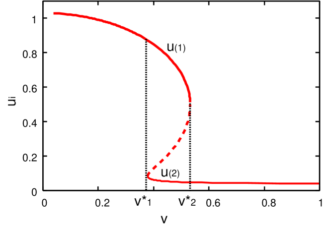
Figure 1:

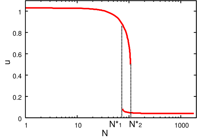
Figure 2:

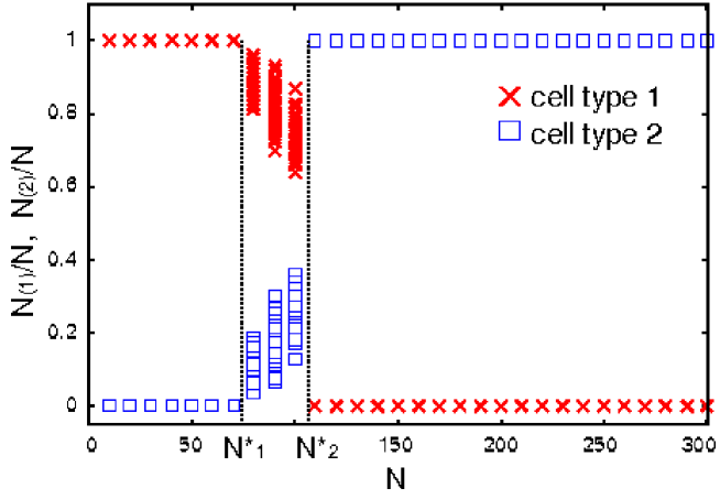
Figure 3:

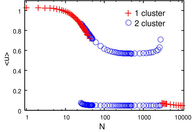
Figure 4:

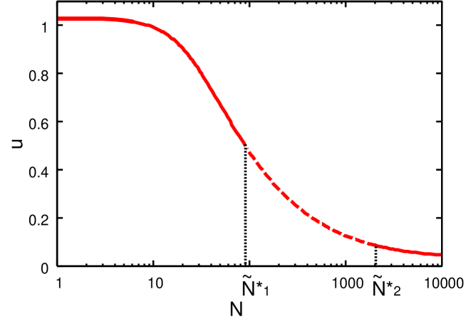
Figure 5:

Figure 6:

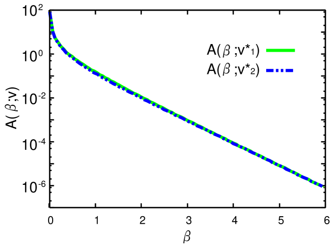
Figure 7:

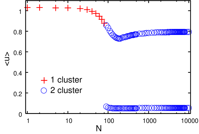
Figure 8:

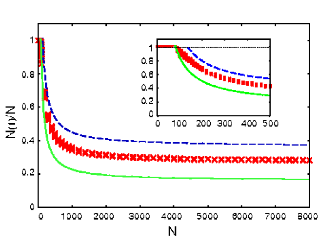
Figure 9:

References

- Adams and Scadden (2006) Adams, G. B., Scadden, D. T., 2006. The hematopoietic stem cell in its place. Nat. Immunol. 7, 333–337.
- Alvarez-Curto et al. (2007) Alvarez-Curto, E., Saran, S., Meima, M., Zobel, J., Scott, C., Schaap, P., 2007. cAMP production by adenylyl cyclase G induces prespore differentiation in Dicyostelium slugs. Development 134, 959–966.
- Ben-Tabou de-Leon and Davidson (2007) Ben-Tabou de-Leon, S., Davidson, E. H., 2007. Gene regulation: Gene control network in development. Annu. Rev. Biophys. Biomol. Struct. 36, 191–212.
- Calvi (2006) Calvi, L. M., 2006. Osteoblastic activation in the hematopoietic stem cell niche. Ann. N. Y. Acad. Sci. 1068, 477–488.
- E. H. Davidson et al. (2002) E. H. Davidson et al., 2002. A genomic regulatory network for development. Science 295, 1669–1678.
- Ferrell Jr. and Machleder (1998) Ferrell Jr., J. E., Machleder, E. M., 1998. The biochemical basis of an all-or-none cell fate switch in Xenopus oocytes. Science 280, 895–898.
- Furusawa and Kaneko (1998) Furusawa, C., Kaneko, K., 1998. Emergence of rules in cell society: Differentiation, hierarchy, and stability. Bull. Math. Biol. 60, 659–687.
- Furusawa and Kaneko (2001) Furusawa, C., Kaneko, K., 2001. Theory of robustness of irreversible differentiation in a stem cell system: Chaos hypothesis. J. Theor. Biol. 209, 395–416.
- García-Ojalvo et al. (2004) García-Ojalvo, J., Elowitz, M. B., Strogatz, S. H., 2004. Modeling a synthetic multicellular clock: Repressilators coupled by quorum sensing. Proc. Natl. Acad. Sci. USA 101, 10955–10960.
- Greenwald and Rubin (1992) Greenwald, I., Rubin, G. M., 1992. Making a difference: the role of cell-cell interactions in establishing separate identities for equivalent cells. Cell 68, 271–281.
- Gurdon et al. (1993) Gurdon, J. B., Lemaire, P., Kato, K., 1993. Community effects and related phenomena in development. Cell 75, 831–834.
- Hartley et al. (1996) Hartley, R. S., Rempel, R. E., Maller, J. L., 1996. In vivo regulation of the early embryonic cell cycle in Xenopus. Dev. Biol. 173, 408–419.
- Hopper et al. (1993) Hopper, N. A., Harwood, A. J., Bouzid, S., Véron, M., Williams, J. G., 1993. Activation of the prespore and spore cell pathway of Dictyostelium differentiation by cAMP-dependent protein kinase and evidence for its upstream regulation by ammonia. EMBO J. 12, 2459–2466.
- Imai et al. (2006) Imai, K. S., Levine, M., Satoh, N., Satou, Y., 2006. Regulatory blueprint for a chordate embryo. Science 312, 1183–1187.
- Kaneko and Yomo (1994) Kaneko, K., Yomo, T., 1994. Cell division, differentiation and dynamic clustering. Physica D 75, 89–102.
- Kaneko and Yomo (1997) Kaneko, K., Yomo, T., 1997. Isologous diversification: a theory of cell differentiation. Bull. Math. Biol. 59, 139–196.
- Kaneko and Yomo (1999) Kaneko, K., Yomo, T., 1999. Isologous diversification for robust development of cell society. J. Theor. Biol. 199, 243–256.
- Kay and Thompson (2001) Kay, R. R., Thompson, C. R. L., 2001. Cross-induction of cell types in Dictyostelium: evidence that DIF-1 is made by prespore cells. Development 128, 4959–4966.
- Koseska et al. (2007) Koseska, A., Volkov, E., Zaikin, A., Kurths, J., 2007. Inherent multistability in arrays of autoinducer coupled genetic oscillators. Phys. Rev. E 75, 031916.
- Loose and Patient (2004) Loose, M., Patient, R., 2004. A genetic regulatory network for Xenopus mesendoderm formation. Dev. Biol. 271, 467–478.
- Maamar et al. (2007) Maamar, H., Raj, A., Dubnau, D., 2007. Noise in gene expression determines cell fate in Bacillus subtilis. Science 317, 526–529.
- McMillen et al. (2002) McMillen, D., Kopell, N., Hasty, J., Collins, J. J., 2002. Synchronizing genetic relaxation oscillators by intercell signaling. Proc. Natl. Acad. Sci. USA 99, 679–684.
- Milo et al. (2004) Milo, R., Itzkovitz, S., Kashtan, N., Levitt, R., Shen-Orr, S., Ayzenshtat, I., Sheffer, M., Alon, U., 2004. Superfamilies of evolved and designed networks. Science 303, 1538–1542.
- Milo et al. (2002) Milo, R., Shen-Orr, S., Itzkovitz, S., Kashtan, N., Chklovskii, D., Alon, U., 2002. Network motifs: Simple building blocks of complex networks. Science 298, 824–827.
- Mizuguchi and Sano (1995) Mizuguchi, T., Sano, M., 1995. Proportion regulation of biological cells in globally coupled nonlinear systems. Phys. Rev. Lett. 75, 966–969.
- Novak and Tyson (1993) Novak, B., Tyson, J. J., 1993. Numerical analysis of a comprehensive model of m-phase control in Xenopus oocyte extracts and intact embryos. J. Cell Sci. 106, 1153–1168.
- Oviedo et al. (2003) Oviedo, N. J., Newmark, P. A., Alvarado, A. S., 2003. Allometric scaling and proportion regulation in the freshwater planarian Schmidtea mediterranea. Dev. Dyn. 226, 326–333.
- Radtke et al. (2004) Radtke, F., Wilson, A., Mancini, S. J. C., MacDonald, R., 2004. Notch regulation of lymphocyte development and function. Nat. Immunol. 5, 247–253.
- Ràfols et al. (2000) Ràfols, I., Amagai, A., Maeda, Y., MacWilliams, H. K., Sawada, Y., 2000. Cell type proportioning in Dictyostelium slugs: lack of regulation within a 2.5-fold tolerance range. Differentiation 67, 107–116.
- Sha et al. (2003) Sha, W., Moore, J., Chen, K., Lassaletta, A. D., Chung-Seon Yi, J. J. T., Sible, J. C., 2003. Hysteresis drives cell-cycle transitions in Xenopus laevis egg extracts. Proc. Natl. Acad. Sci. USA 100, 975–980.
- Shen-Orr et al. (2002) Shen-Orr, S. S., Milo, R., Mangan, S., Alon, U., 2002. Network motifs in the transcriptional regulation network of Escherichia coli. Nat. Gen. 31, 64–68.
- Süel et al. (2006) Süel, G. M., García-Ojalvo, J., Liberman, L. M., Elowitz, M. B., 2006. An excitable gene regulatory circuit induces transient cellular differentiation. Nature 440, 545–550.
- Swiers et al. (2006) Swiers, G., Patient, R., Loose, M., 2006. Genetic regulatory networks programming hematopoietic stem cells and erythroid lineage specification. Dev. Biol. 294, 525–540.
- Tyson et al. (2003) Tyson, J. J., Chen, K. C., Novak, B., 2003. Sniffers, buzzers, toggles and blinkers: dynamics of regulatory and signaling pathways in the cell. Curr. Opin. 15, 221–231.
- Ullner et al. (2007) Ullner, E., Zaikin, A., Volkov, E. I., García-Ojalvo, J., 2007. Multistability and clustering in a population of synthetic genetic oscillators via phase-repulsive cell-to-cell communication. Phys. Rev. Lett. 99, 148103.
- Williams (2006) Williams, J. G., 2006. Transcriptional regulation of Dictyostelium pattern formation. EMBO Rep. 7, 694–698.