Transport properties in chaotic and non-chaotic many particle systems

Abstract

Two deterministic models for Brownian motion are investigated by numerical simulations and kinetic theory arguments. The first model consists of a heavy hard disk immersed in a rarefied gas of smaller and lighter hard disks acting as a thermal bath. The second is the same except for the shape of the particles, which is now square. The basic difference in these two systems lies in the interaction: hard-core elastic collisions make the dynamics of the disks chaotic whereas that of squares is not. Remarkably, this difference does not reflect on the transport properties of the two systems: simulations show that the diffusion coefficients, velocity correlations and response functions of the heavy impurity are in agreement with kinetic theory for both the chaotic and non-chaotic model. The relaxation to equilibrium instead is very sensitive to the kind of interactions. These observations are used to think back and discuss some issues connected to chaos, statistical mechanics and diffusion.

Keywords: Brownian motion, transport properties (theory), fluctuations (theory)

1 Introduction

A century after Einstein [1] and Smoluchowski [2] seminal contributions, Brownian motion (BM) and diffusion phenomena remain an active subject of research. Statistical mechanics, since its foundation, has been operating an elegant synthesis between the microscopic dynamical laws and the macroscopic properties of a system. In this context, Brownian motion is a paradigmatic example of this modus operandi.

In the statistical mechanics framework, the minimal condition needed by microscopic dynamics for macroscopic diffusion can be identified in the presence of a mechanism leading to velocity decorrelation – memory loss. In the effort of interpreting BM and non-equilibrium transport in the light of modern dynamical systems theory, it thus comes rather natural to identify in the chaotic character of microscopic dynamics the main candidate to explain macroscopic transport. The instabilities of chaotic evolutions typically produce irregular trajectories resembling Brownian motions and supply a simple mechanism for memory loss. Indeed large scale diffusion has been found in simple low dimensional chaotic systems [3, 4, 5]. This picture received theoretical support from the existence, in some systems, of remarkable quantitative relations between macroscopic transport coefficients – such as diffusivity, thermal and electrical conductivity –, and microscopic chaos indicators – such as the Lyapunov exponents and the Kolmogorov-Sinai entropy –, see e.g. [6, 7, 8, 9, 10].

On the other hand, non-chaotic models generating diffusion have been proposed [11, 12, 13, 14] raising some doubts on the actual role of chaos for diffusion. However, these models, representing possibly the most elementary examples of diffusion without chaos, seem to be rather artificial: involve few degrees of freedom, often the presence of quenched randomness is needed together with the fine tuning of some parameters, e.g., for the suppression of periodic orbits [14]. Their relevance to statistical mechanics is thus not obvious. It is worth remarking that questions about the relevance of chaos have been recently raised also in the (related) context of thermal conduction problems [15], where non-chaotic models for heat transport were proposed and investigated [16, 17, 18, 19].

It should be remarked that the above systems are non-chaotic in the sense that the Lyapunov spectrum is non-positive. However, there are well known examples of Lyapunov stable systems that display non trivial behaviours [11, 14, 16, 17, 18, 19, 20]. In the presence of dynamical randomness without the sensitivity to initial condition, as in quantum mechanics, an alternative definition of ”chaos” or ”randomness” has been proposed in terms of the positiveness of the Kolmogorov-Sinai entropy [21]. In classical systems with a finite number of degrees of freedom, as consequence of the Pesin’s formula, the two definitions coincide. However, the proposal of Ref. [21] is an interesting open possibility for quantum and classical systems in the limit of infinite number of degrees of freedom.

It is far from trivial to the establish the role of chaos to macroscopic transport properties. The problem is actually more general as chaos (in the above wider definition) had been often invoked to justify the whole statistical mechanics apparatus [9, 10] and to explain the irreversibility of macroscopic processes [22]. Such viewpoint coexists with the “more traditional” approach of Boltzmann, which stresses the role of the many degrees of freedom and is mathematically supported by the results of Khinchin [23], Mazur and van der Linden [24] (see also Bricmont [25] and references therein).

This paper aims to discuss the role of chaos in the context of diffusion, thus we compare a chaotic and a non-chaotic many degrees of freedom system, providing two distinct deterministic models for BM. Both models consist of rarefied gas of hard particles surrounding a larger and heavier particle, in the following referred to as colloidal particle (or colloid for brevity), impurity or test particle. As an effect of the large number of collisions, the deterministic motion of such an impurity behaves as a BM at long times (i.e. much larger than the collision time) provided its mass is much larger than that of the lighter gas particles. The latter condition ensures a scale separation between the gas and impurity dynamics. The asymptotic convergence to a BM was proved for an infinite one dimensional system of hard-core particles [26] and, later, in three dimensions [27].

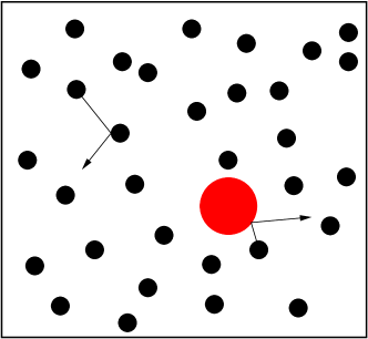
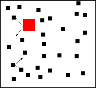
Figure 1: Schematic illustration of two models used to discuss the mechanical diffusion: (left) hard disks and (right) hard parallel (non rotating) squares. The colloidal particle is displayed in red.

The first model consists of $N$ hard disks surrounding a larger and heavier disk as sketched in Fig. 1 (left). Particle interactions occur via binary elastic, hard-core collisions which, due to convex shape of the disk, lead to chaotic trajectories (i.e. exponential separation among initially close trajectories). In the following, this hard disk model will be denoted by the acronym HD.

The second model, illustrated in Fig. 1 (right), consists of a gas of $N$ hard (non-rotating) parallel squares (HPS) surrounding a larger and heavier square particle. In this case, binary hard-core elastic collisions are not central and conserve the initial parallel orientation of the squares. Unlike HD, the resulting dynamics is non-chaotic. This model is not new, the case of a HPS gas with identical particles (without the impurity) has been studied both in terms of molecular dynamics and kinetic theory by Frisch and coworkers [28, 29, 30, 31]. It constitutes an interesting statistical mechanics system characterized by the presence of an infinite number of integrals of motion, preventing the system from being ergodic. Remarkably, in spite of such a pathology, the HPS gas gives rise to, e.g., phase transitions and transport properties as in the HD gas which, on the contrary, possesses ergodic and mixing properties.

The colloid can be seen as a test particle to probe the transport properties of both HPS and HD. Notwithstanding the intrinsic difference in their dynamics, chaotic for HD and non-chaotic for HPS, their macroscopic diffusion properties are remarkably similar, as confirmed by the analysis of the velocity-velocity correlations, connected to diffusion via the Green-Kubo formula [32, 33]. Measurements of the response function of the velocity of the colloid and of gas particles to small perturbations confirm that the non-chaotic nature of HPS does not influence either the diffusion or the validity of the Fluctuation Dissipation Theorem (FDT).

To discriminate the behavior of HPS from HD model one has to look at the relaxation to equilibrium, when the initial state is very far from it. For square particles relaxation properties crucially depend on the presence of the impurity, which induces a sort of “effective interaction” among the gas particles and allows the system to equilibrate to the Maxwell-Boltzmann distribution. Since collisions simply reshuffle the velocity components among the particles, preserving the initial velocity distribution, without the colloidal particle relaxation to Maxwell-Boltzmann is not possible. In spite of such a constraint, self-diffusion and other statistical mechanics behaviors can still be found [28, 29, 30, 31] (see also Sect. 3). In the presence of the colloid, a signature of such a pathology survives: the relaxation time $\mathcal{T}_{r}$ strongly depends on the mass of the impurity, whilst in HD it is independent of it. Moreover, ergodicity is not fully recovered being the exchanges between the $x$ and $y$ components of the velocity forbidden.

The paper is organized as follows. Sect. 2 introduces the two models. In Sect. 3, the numerical results for the diffusion coefficient, self-diffusion and velocity auto-correlation function are presented. In Sect. 4, the relaxation properties of HPS and HD close-to and far-from equilibrium are analyzed. Sect. 5 concludes the paper with a discussion of the relation among chaos, statistical mechanics and diffusion based on our results. In the Appendix, a kinetic theory derivation of the diffusion constants for both models is presented in the very dilute limit.

2 Deterministic many particle models for diffusion

In the spirit of Smoluchovski’s approach [2], it is natural to introduce a mechanical model for BM based on the dynamics of a macroscopically small but microscopically large heavy impurity colliding with many lighter particles. The large mass and size with respect to the gas particles allows for a separation of time scales so that the velocity of such an impurity is expected to follow a Langevin equation. The collisions with the gas provide both the friction and the stochastic kicking to the colloid [34]. Here, we focus on two different models in two dimensions.

2.1 Hard disks model (HD)

We consider $N$ hard disks of radius $r$ and mass $m$ plus an impurity consisting in another disk of radius $R>r$ and mass $M>m$, as in Fig. 1(left). All particles are in a square box of side $L$, with periodic boundary conditions. Crucial parameters are the number density $\rho=N/L^{2}$ and the volume fraction $\psi=N\pi r^{2}/L^{2}$. In the following, we shall always consider very dilute systems ($\psi\ll 1$) so that the properties of the system will be akin to those of a rarefied gas.

The kinetic energy coincides with the total energy $H$

$$H=\sum_{j=1}^{N}\frac{{\bm{p}}_{j}^{2}}{2m}+\frac{{\bm{P}}^{2}}{2M}\equiv\sum_{j=1}^{N+1}\frac{{\bm{p}}_{j}^{2}}{2m_{j}}\,,$$ (1)

and is conserved. In the second equality of Eq. (1) we adopt the convention that $i\!=\!N\!+\!1$ indicates the colloid, i.e. ${\bm{p}}_{N\!+\!1}\!=\!\bm{P}$ and $m_{N\!+\!1}\!=\!M$ while $m_{i}\!=\!m$ for $i=1,...,N$. Similarly, for the coordinates, we use either $\bm{q}_{i}=(x_{i},y_{i})$ ($i=1,\dots,N$) for the gas particles and $\bm{Q}=(X,Y)$ for the mass impurity, or ${\bm{q}}_{j}$ for $j=1,\dots N+1$ with ${\bm{q}}_{N+1}=\bm{Q}$. Of course, if $r=R$ and $m=M$, Eq. (1) reduces to a system of $N+1$ identical hard disks, which has been thoroughly investigated by accurate computer simulations [35] and theoretically in terms of kinetic theory of gases (see e.g. [9, 36] and references therein) in a variety of regimes.

Each particle moves with constant velocity till it collides with another particle, event at which the velocities are updated according to the elastic collisions rule

$${\bm{p}}_{i}^{\prime}={\bm{p}}_{i}+\frac{2m_{i}m_{j}}{m_{i}+m_{j}}({\bm{g}}_{ij}\cdot\hat{\bm{e}}_{ij})\hat{\bm{e}}_{ij}\quad\textrm{and}\quad{\bm{p}}_{j}^{\prime}={\bm{p}}_{j}-\frac{2m_{i}m_{j}}{m_{i}+m_{j}}({\bm{g}}_{ij}\cdot\hat{\bm{e}}_{ij})\hat{\bm{e}}_{ij}$$ (2)

where post-collision quantities are primed, and $\bm{g}_{ij}=\bm{p}_{i}/m_{i}-\bm{p}_{j}/m_{j}=\bm{v}_{i}-\bm{v}_{j}$ is the precollisional relative velocity. The unitary vector $\hat{\bm{e}}_{ij}$, oriented as $i\to j$, connects the centers of the two disks at contact.

The model (1) simplifies for two asymptotics: for $M/m\to 0$, it approaches the Lorentz-gas model [37], the impurity is much faster than the (now heavier) gas particles which can be treated as immobile obstacles; for $R/r\to\infty$, the Rayleigh-flight model is recovered if the $N$ small disks are very dilute so that most of collisions involve the impurity. In these two limits, kinetic theory allows for analytical approximation of the maximum Lyapunov exponent in terms of the system parameters [38].

Here, being interested in Brownian motion, we consider situations in which $R\gg r$ and $M\gg m$. In such a limit, thanks to the large time scale separation between the impurity and gas particles motions, it is reasonable to assume that each velocity component $V$ of the colloid follows a Langevin equation (we set $k_{B}=1$)

$$\frac{dV}{dt}=-\gamma V+\sqrt{2\gamma\frac{T}{M}}\,\eta\,,$$ (3)

where $T$ is the gas temperature, and $\eta(t)$ a zero mean Gaussian process with correlation $\langle\eta(t)\eta(t^{\prime})\rangle=\delta(t-t^{\prime})$. Of course, Eq. (3) describes the effective dynamics of the impurity for times much larger than the average collision time with the gas particles [34, 26, 27]. The friction constant $\gamma$ sets the decay of velocity-velocity correlation function

$$C_{V}(t)=\langle V(t)V(0)\rangle=\langle V^{2}\rangle\mbox{e}^{-\gamma t}=\frac{T}{M}\textrm{e}^{-\gamma t}\,,$$ (4)

where brackets indicate time or ensemble averages. By standard kinetic-theory computation (see Eq. (19) where also corrections in $r/R$ and $m/M$ are taken into account) one has

$$\gamma=2\sqrt{2\pi}\,\frac{\rho R\sqrt{mT}}{M}\,.$$ (5)

Now, thanks to the Green-Kubo relation, linking the auto-correlation function to the diffusion coefficient $D$

$$D=\int_{0}^{\infty}\langle V(t)V(0)\rangle dt=\frac{\langle V^{2}\rangle}{\gamma}=\frac{T}{M\gamma}\,,$$ (6)

it is straightforward to derive the diffusion constant of the colloidal particle

$$D_{c}=\lim_{t\to\infty}\frac{1}{2t}\langle[X(t)-X(0)]^{2}\rangle=\frac{1}{2\sqrt{2\pi}}\,\frac{1}{\rho R}\sqrt{\frac{T}{m}}\,.$$ (7)

Notice that $D_{c}$ is proportional to $\sqrt{T}$ and not to $T$ as in liquids. This comes from the fact that in liquids the friction is temperature independent, while in rarefied gases it is proportional to the square root of the temperature.

Another interesting quantity, well defined both in the presence or absence of the impurity, is the self-diffusion coefficient $D_{g}$ of a tagged gas particle. This is an important transport coefficient associated with the gas density field evolution. Previous investigations of hard disks and spheres models studied in details such a quantity as well as other transport coefficients (e.g., viscosity) at varying the parameters of the problem. In the dilute limit, the particle self-diffusion coefficient takes the form [9]:

$$D_{g}=\lim_{t\to\infty}{1\over 2t}\langle[x(t)-x(0)]^{2}\rangle=\frac{1}{4\sqrt{\pi}}\frac{1}{\rho r}\sqrt{\frac{T}{m}}\,,$$ (8)

where $x$ indicates the $x$-component of the position of a tagged gas particle. At high volume fractions, corrections to the formula must be considered. Although the expression is formally similar to (7), only the prefactors change, the Langevin description (3) does not apply in this case due to the absence of time scale separation. One has to take care to work in conditions in which the coefficient (8) is insensitive to the presence of the impurity, so that it can be considered as a small perturbation.

Before passing to the other model, it is important to give a warning. In two dimensions, as here, it is long known [39, 40] that the gas velocity auto-correlation function develops small, slowly decaying tails. In principle, this may lead to an ill defined diffusion coefficient. However, when $\psi\to 0$ this problem becomes relevant only for enormously long times [41]. Therefore, disregarding this issue is justified from the practical point of view and we will ignore it in the following.

2.2 Hard parallel squares (HPS)

We now consider a different model of hard-core particles in which the $N$ gas disks are replaced by $N$ squares of side $2r$ and mass $m$ plus a square colloid of side $2R$ ($R>r$) and mass $M>m$, contained in a box of size $L\times L$ with periodic boundary conditions.

At the initial time, the sides of all squares are parallel (see Fig 1(right)), and such parallelism is conserved (no rotation) by the elastic, hard-core collisions, which are now not central and amount to equal angle reflection against parallel sides. The Hamiltonian (1) is still describing the system, and the collision rule (2) are replaced by

$${\bm{p}}_{i}^{\prime}={\bm{p}}_{i}+\frac{2m_{i}m_{j}}{m_{i}+m_{j}}({\bm{g}}_{ij}\cdot\hat{\bm{n}}_{ij})\hat{\bm{n}}_{ij}\quad\textrm{and}\quad{\bm{p}}_{j}^{\prime}={\bm{p}}_{j}-\frac{2m_{i}m_{j}}{m_{i}+m_{j}}({\bm{g}}_{ij}\cdot\hat{\bm{n}}_{ij})\hat{\bm{n}}_{ij}\,,$$ (9)

where ${\bm{g}}_{ij}$ is the relative velocity, and the unitary vector $\hat{\bm{n}}_{ij}$ is directed as the normal to the colliding sides, that is, either along the $x$ or $y$ axes. At variance with the HD, the HPS model is not a mechanical system as its evolution does not follow the Newtonian dynamics, because of the constraint keeping the parallelism among the square sides. Since the collision rules (9) are linear, the evolution law for the tangent vector coincides with that of the system and the Lyapunov exponents are all equal to zero. Therefore, unlike the case of disks, the system is non-chaotic, although the presence of the corners may induce non-linear instabilities, producing a defocusing for non-infinitesimal displacement among two trajectories.

In the absence of the impurity the considered system reduces to $N$ identical parallel squares, which was studied by Frisch and coworkers [28, 29, 30, 31] for its peculiar properties. This system is indeed interesting under several aspects. First of all, due the rules of interaction (9), colliding particle pairs simply exchange their velocities along the direction of impact: similarly to $1$d hard rods a collision event corresponds to a relabeling of particles, though in the $2d$ case as here the relabeling is only for one component of the velocity. This implies that all velocity moments are conserved separately for the two components. It thus follows that a velocity probability distribution function (pdf), which is initially factorized $P(v_{x},v_{y};t=0)=p(v_{x})p(v_{y})$, is preserved by the time evolution. In other words, unlike HD, the system is non-ergodic and the pdf of the velocities cannot relax to the Maxwell-Boltzmann distribution. However, if the initial distribution is not factorized, it will factorize $P(v_{x},v_{y};t\to\infty)=f(v_{x})g(v_{y})$ with $g(v_{x})=\int dv_{y}P(v_{x},v_{y};t=0)$ and $g(v_{y})=\int dv_{x}P(v_{x},v_{y};t=0)$. Indeed the relabeling induced by the collisions decorrelate the $x$ and $y$ components.

In spite of these pathologies, simulations [28] and kinetic theory computations [29] show that this non-ergodic system possesses many properties akin to those of the HD, which instead is typically considered to be ergodic and mixing. For instance, transport properties are well defined and in the dilute limit. The self-diffusion coefficient for an initial Maxwell-Boltzmann distribution can be computed [28]

$$D_{g}=\frac{\sqrt{\pi}}{16}\frac{1}{\rho r}\sqrt{\frac{T}{m}}\,.$$ (10)

Moreover, phase transitions similar to those found in HD can be observed for suitable values of the volume fraction $\psi=N4r^{2}/L^{2}$ [29].

When the impurity is present the situation changes. Due to the mass difference ($m\neq M$), many conserved quantities are destroyed and collisions can change the velocities pdf: relaxation to Maxwell-Boltzmann distribution is now possible. Essentially the impurity allows for an “effective interaction” as e.g. in [42]. However, ergodicity is not fully recovered: it is clear that, due to the collision rule, no mixing between the velocities along $x$ and $y$ is possible. Meaning that $E_{x}=\sum_{i=1}^{N+1}{p}_{xi}^{2}/2m_{i}$ and $E_{y}=\sum_{i=1}^{N+1}{p}_{yi}^{2}/2m_{i}$ are separately conserved. We shall always work in isotropic conditions, i.e. with initial velocity pdf such that $E_{x}=E_{y}$

In such a condition, being an equilibrium distribution well defined, we can still consider the limits $R\gg r$ and $M\gg m$ and study the BM of the impurity. From kinetic theory (see Eq. (22) in the Appendix), one can compute the friction coefficient

$$\gamma=8\sqrt{\frac{2}{\pi}}\frac{\sqrt{m}\rho R\sqrt{T}}{M}\,,$$ (11)

and therefore the diffusion constant

$$D_{c}=\frac{\sqrt{\pi}}{8\sqrt{2}}\frac{1}{\rho R}\sqrt{\frac{T}{m}}\,\,.$$ (12)

Comparing the above expression with (7) reveals that the only difference lies in a numerical prefactor which takes into account the different geometries of the particles.

3 Transport Properties

Let us now investigate, by means of numerical simulations, the transport properties (diffusion of the impurity and self-diffusion of tagged gas particles) in HD and HPS models both in the presence and absence of the impurity.

Before discussing the results, we briefly summarize the numerical methods employed. For both HPS and HD, we used an event driven algorithm with the minimum image convention [35]. All simulations refer to the rarefied case. After several tests we fixed $\rho=N/L^{2}=10$ and solid fraction $\psi\approx\mathcal{O}(10^{-3})$, so that we can neglect all known corrections to the transport coefficients [36]. The diffusion constants are then measured in terms of the mean square displacement in the $x$ and $y$ direction for both the colloid and tagged gas particles, see Eqs. (7) and (8). Working in isotropic conditions, the horizontal and vertical diffusion coefficient are equal, allowing us to average over the two components for increasing statistics. Averages have been computed over $\mathcal{N}$ time windows in a long run. The diffusion constant $D_{c}$ is thus obtained by looking at

$$\langle[\Delta Q(t)]^{2}\rangle=\frac{1}{\mathcal{N}}\sum_{k=1}^{\mathcal{N}}[Q(t+t_{k})-Q(t_{k})]^{2}\;\approx 2D_{c}t\,,$$ (13)

where $Q=X,Y$ represents any of the components of the particle position, and $0\leq t\leq(t_{k+1}-t_{k})$. The length of the window $t_{k+1}-t_{k}$ is chosen long enough to observe a diffusive regime over about two decades. For the self-diffusion we proceeded similarly, but working on the gas particle positions, $q_{i}=x_{i},y_{i}$. Being all gas particles equivalent, we average over them

$$\langle[\Delta q(t)]^{2}\rangle\!=\!\frac{1}{N\mathcal{N}}\sum_{k=1}^{\mathcal{N}}\sum_{i=1}^{N}[q_{i}(t+t_{k})-q_{i}(t_{k})]^{2}\;\approx 2D_{g}t\,$$ (14)

with abuse of notation the same brackets as in (13) are used though in (14) the average over all particles is also performed. HD and HPS simulations differ only for the collision rules. While computing the average displacements we also computed the velocity auto-correlation functions for both the colloid and gas particles $C_{V}(t)$ and $C_{v}(t)$. The averages have been performed, as for the displacements, over different time windows and, for the gas, also over all particles.

We work with a single impurity with $R=10r$ and $M=20m$ (tests with different sizes and masses have been performed). Due to the necessity of averaging over many, typically $\mathcal{N}=10^{3}$, time windows we employ a not too large number of gas particles ($N=300$, tests with $N=1000$ have been done). Using this relatively low number of particles and the mass ratio $M/m=20$ requires to take into account finite size corrections. Indeed the constraints of energy and momentum conservation (the latter ensured by the periodic boundary conditions) are known to cause a breakdown of the energy equipartition for simulations with non-equal mass particles [43, 44].

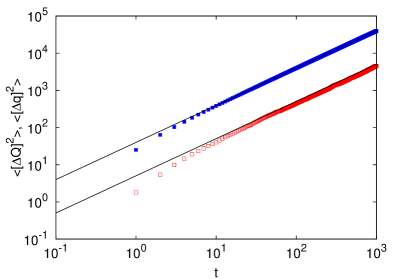
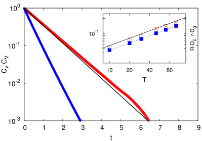
  (a)                                                                (b)

Figure 2: (a) Mean square displacement for the colloid $\langle[\Delta Q(t)]^{2}\rangle$ (red) and tagged gas particles $\langle[\Delta q(t)]^{2}\rangle$ (blue) vs time for HD. The straight lines show the expectations (7) and (8), respectively. The temperature is set to $T=50$. (b) Velocity auto-correlation for colloid $C_{V}(t)$ (red) and gas particles $C_{v}(t)$ (blue) measured in the same simulation as (a). The straight line has a slope given by the friction constant (5). Inset: Normalized diffusion constants $RD_{c}$ and $rD_{g}$ vs $T$. Solid and dotted lines correspond to the expectation (7) and (8) with the finite sample size corrections included [43, 44]. $N=300$ gas particles of radius $r=0.005$ and mass $m=1$ have been used, with number density $\rho=10$, for the impurity $R=10r$ and $M=20m$. Averages are performed over $\mathcal{N}=1000$ time windows. Simulations on a shorter time scale with $N=1000$ particles give the same result within statistical errors. Notice that the self diffusion is by definition the results of a further average over the number of gas particles, thus its statistics is much improved than $D_{c}$ implying lower statistical errors.

We are now ready to discuss the results. Let us start from Fig. 2a where we show the data for the diffusion and velocity correlation of the impurity and tagged gas particles in the case of hard disks. Although the diffusive properties of HD have been thoroughly studied in the literature, they serve for comparison with HPS, presented below. As one can see, the diffusive scaling extends over about two decades allowing for a good estimate of the diffusion coefficients, which are in agreement with the expectation (7) and (8), see also the inset in Fig. 2b. The auto-correlation functions $C_{V}$ and $C_{v}$ (shown in Fig. 2b) display an exponential decay. For the colloid the decay time is in agreement with the friction constant (5), making the approximation of the colloid evolution in terms of a Langevin equation meaningful.

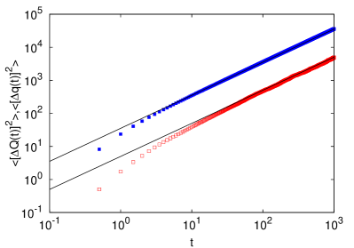
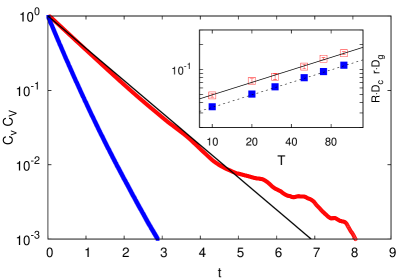
  (a)                                                                (b)

Figure 3: Same of Fig. 2 for HPS. The size of the particles has been chosen so to have the same area of the disks.

We now consider the case of $N$ parallel squares with a mass impurity. As discussed in the previous section, the presence of the colloid allows for the existence of an equilibrium state characterized by the Maxwell-Boltzmann distribution for the particle velocities. However, unlike HD, the system is non-chaotic. Moreover, ergodicity is broken and there is no mixing between the horizontal and vertical components. As Fig. 3a clearly shows the transport properties of HPS are well defined, the colloidal particle and tagged gas particles diffuse with coefficients as given by Eq. (12) and (10), respectively; see also inset in Fig. 3b. Moreover, the system loses memory as both the velocity auto-correlation function of the impurity and gas particles decay exponentially (Fig. 3b). At a first sight, the agreement of the self-diffusion constant with (10) may appear strange. Indeed, the formula derived by Frisch and collaborators [28] refers to a gas of identical particles, where no equilibration occurs. However, Eq. (12) was obtained assuming a Gaussian distribution for the velocities, here always realized thanks to the presence of the impurity which allows for Maxwell-Boltzmann distribution.

We consider now the model in which no impurity is present, previously studied by Frisch and collaborators [29, 30]. As stressed above, in such a case HD and HPS (i.e. chaotic and non-chaotic particle systems) are conceptually very different: while HD remains a well defined statistical mechanics system with relaxation to an equilibrium state independent from the initial conditions, HPS never reaches equilibrium, the initial velocity distribution remains unchanged with time. Nevertheless both systems display well defined transport properties.

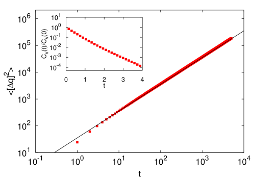
Figure 4: (a) $\langle\Delta q^{2}(t)\rangle$ vs $t$ for a gas of $N=300$ hard parallel squares with size as in Fig. 3 and with a Gaussian velocity distribution at temperature $T=50$ and number density $\rho=10$. Inset: velocity auto-correlation function. With $N=1000$ we obtained indistinguishable results.

By computing $D_{g}$ for HD in the same conditions as Fig. 2a we checked whether the value of $D_{g}$ agrees with its measurement done in the presence of the colloid. We actually found a perfect agreement, within errors, between the two measurements (not shown). This confirms a posteriori that the colloid can be considered a small perturbation for the gas without important consequences for the transport properties of the HD gas. More interesting is to investigate the case of squares.

In Fig. 4, we show $D_{g}$ for a gas of equal hard squares with Gaussian initial distribution having the same temperature as in the simulations with the impurity: the diffusive behavior is again a robust well defined property. It is worth underlining the following points. First, a diffusive behavior is observed also also in the absence of relaxation to a statistically steady state. Second, the value of $D_{g}$ matches the theoretical value obtained by Frisch [28] and is in perfect agreement, within errorbars, with the equivalent quantity obtained in the presence of the impurity. Third, the velocity-velocity correlation function, shown in the inset, decorrelates exponentially with a good degree of approximation.

The presence of diffusive behaviour in non-chaotic systems is not new. Models consisting of non interacting particles has been already considered in Refs. [12, 13]. However, such models, though interesting from a dynamical system point of view, consist of independent particles and thus are somehow far from a statistical mechanics perspective. The HPS system here investigated is non-chaotic but having many degrees of freedom in interaction it constitutes a valuable statistical mechanical system.

We conclude this section by stressing that, although the presence of the colloid changes conceptually the properties of the system, transport properties in the presence or absence of the impurity are quantitatively the same, provided the Gaussian distribution is chosen. This means that, at least, for transport properties the colloid can be considered as a small perturbation to the system, but for a non generic state.

4 Relaxation Properties

The analysis of the relaxation processes associated with spontaneous or induced statistical fluctuations represents the classical approach to probe the macrostates explored by a system. For instance, Fluctuation Dissipation Theorems (FDT) [33], relating the behavior of spontaneous fluctuations at equilibrium to the average response of a system to infinitesimal perturbations, establish a connection between equilibrium (correlation functions) and non-equilibrium (response functions) quantities. We carried out a set of simulations to determine the relaxation properties of the system both close-to the equilibrium state, characterized by a Maxwell-Boltzmann distribution, and far-from it (e.g., starting from a uniform distribution) to probe the possible influence of chaos on the statistical properties.

4.1 Close to equilibrium

To gain information about transport properties by studying the relaxation to equilibrium it is useful to introduce the response function to small impulsive perturbations applied to a component $V$ of the velocity of the impurity. This can be obtained, e.g., by applying a force $f(t)=F\delta(t)$ which acts only at $t=0$ with $F\ll 1$. The result of $f(t)$ is to cause an instantaneous (very small) variation of the velocity $V(0)\to V(0)+\delta V_{0}$, with $\delta V_{0}=F/M$. One can thus define the average response function as $R_{V}(t)=\langle\delta V(t)\rangle_{e}/\delta V_{0}$, where $\langle[\dots]\rangle_{e}$ denotes an ensemble average at fixed time in the presence of an impulsive perturbation. The response $R_{V}(t)$ bears important information on the transport properties of the system being. Indeed, if the velocity distribution is Gaussian the classical FDT relation [33] tells us that $R_{V}(t)$ coincides with the normalized velocity correlation function

$$R_{V}(t)=\frac{C_{V}(t)}{C_{V}(0)}\,.$$ (15)

This can be seen as the differential form of the Einstein relation connecting the asymptotic speed of the particle to the mobility under the effect of an infinitesimally small force. In the following, we present the measurement of the response function $R_{V}(t)$, which will be compared with the correlation $C_{V}(t)$ to test whether FDT holds. Similarly, we analyze also the response function of a tagged gas particle $R_{V}(t)$ when the impurity is absent.

In order to numerically compute the response function, we adopted the following protocol. Consider a system HPS or HD in the presence of the colloidal particle and let it evolve till the equilibrium state is reached. At this time, that we call $t=0$, the velocity of the colloidal particle is perturbed by a small amount $V(0)\to V(0)+\delta V_{0}$. In principle, the perturbation should be infinitesimal (i.e. $\delta V_{0}\to 0$). This is however infeasible in practical computations, we then considered three different perturbation values defined in fraction of the root mean square velocity $\delta V_{0}=\alpha\sqrt{T/M}$ with $\alpha=0.02,0.05$ and $\alpha=0.1$. In this way, comparing the different numerical experiments, we can test a posteriori the validity of the linear response theory. This small perturbation on the velocity is expected to be re-adsorbed, meaning that the velocity of the impurity should, after a while, assume values drawn from the equilibrium distribution. The procedure is thus repeated for many (typically $10^{4}-10^{5}$) times. The time history of the colloidal particle $V(t)$ is followed in each experiment so to obtain its average evolution $\langle V(t)\rangle_{e}$, from which the response function $R_{V}(t)$ can be defined as

$$R_{V}(t)=\frac{\langle V(t)\rangle_{e}}{\delta V_{0}}\,,$$ (16)

note that we used that $\langle V(0)\rangle_{e}=0$.

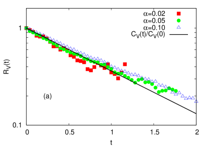
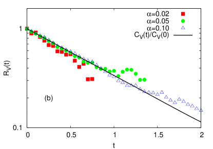
Figure 5: (a) $R_{V}(t)$ vs $t$ measured for $\delta V_{0}=\alpha\sqrt{T/M}$ with $\alpha=0.02,0.05,0.1$ as in the legend and $C_{V}(t)/C_{V}(0)$ (solid line) computed in the same conditions. The parameters are as in Fig. 2 with $T=50$. Note the good collapse, within statistical errors, of the response functions for $\alpha=0.02$ and $\alpha=0.05$ and the correlation function. Deviations can be appreciated for $\alpha=0.1$ (presumably for such a value of the perturbation one exits the linear response regime). (b) the same of (a) for HPS system with parameters as in Fig. 3, the agreement between the decay of the correlation and the response function is also in this case very good. For both (a) and (b), the three curves have different length because decreasing the initial perturbation value the signal is spoiled by noise at earlier times.

Equation (16) has been verified in our simulations for both HPS and HD, and the comparison between the numerical results is shown in Fig. 5. One should notice first that for both HD and HPS the response measured for different perturbations superimpose, meaning that we are in the linear response regime. Moreover, the fair superposition of the exponential decays of $C_{V}(t)$ and $R_{V}(t)$, up to statistical errors, constitutes the numerical evidence for both systems to obey FDT relation.

The conclusion that can be drawn is that whenever the chaotic HD and the non-chaotic HPS are prepared into an equilibrium state compatible with the thermodynamic parameters $T$ and $\rho$, the behavior of $R_{V}(t)$ does not reveal any difference between the two systems.

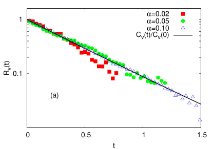
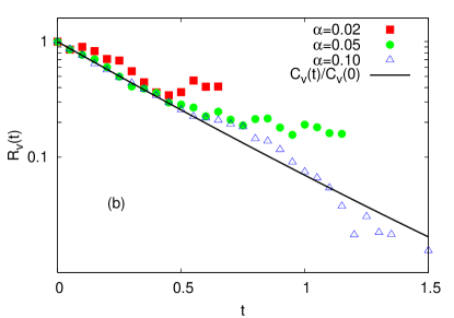
Figure 6: The same of Fig. 5(a) showing the FDT relation for the HD (a) and HPS (b) gas particle (in the absence of the impurity). For HPS the initial distribution of the gas velocities was chosen Gaussian with temperature $T=50$ so to compare with the correlation function as measured in Fig. 4.

The above procedure can be applied to a tagged particle so to define the response for gas particles $R_{v}(t)$ which is connected to the correlation function $C_{v}(t)$. We perform such a measurement for the system of HD and HPS without the impurity. Being the perturbation very small the measurement is still meaningful though the system is not equilibrating.

Figure 6 shows the average response functions for a tagged particle in both HD and HPS, together with the comparison with the correlation functions. There is a fair agreement between $R_{v}(t)$ and $C_{v}(t)/C_{v}(0)$ for both HD and HPS models. Of course, in the case of the HPS the origin of the validity of a FDT relation cannot be ascribed to the presence of chaos. Clearly it can only come from the presence of many degrees of freedom and should have a probabilistic origin.

4.2 Far-from equilibrium

We consider now the case of relaxation when the system is prepared into a state far-form equilibrium, for which the difference between the two models becomes evident. This can be understood from the outset by recalling that HPS systems with identical squares cannot relax due to the collision rules that merely relabel the velocity components. Unlike HPS, hard disks collisions, also thanks to chaos, mix the velocity components at each impact and allow for a fast relaxation to a Maxwell-Boltzmann distribution.

When the colloid is introduced, relaxation to equilibrium becomes possible also in HPS because impacts against the impurity break the relabeling process and provide a mechanism for the transfer of energy (at least, separately for the $x$ or $y$ components which do not mix), this is similar to the problem of the adiabatic piston considered in Ref. [42]. However, since only collisions with the impurity contribute to the relaxation process of the gas, the time-scale for reaching the equilibrium state crucially depends on its mass $M$ and size $R$. This contrasts with the HD model, for which the time scale of relaxation is essentially unaffected by the characteristics and/or the presence of the colloid.

In our simulations, we prepare the HD or HPS gas in a state with a spatially homogeneous distribution of particles and flat velocity distribution, i.e. $P(v_{x},v_{y})=g(v_{x})g(v_{y})$ with $g(v)=1/(2v_{0})$ for $|v|<v_{0}$ and zero elsewhere. The value of $v_{0}$ is fixed by imposing the temperature $T$ of the system, i.e. $v_{0}^{2}/6=\int dvg(v)v^{2}=T/m$. The colloidal particle is initialized with random velocity extracted from the same distribution. The system is then let evolve under the event driven dynamics, and the velocity pdf monitored by computing

$$\mathcal{K}(t)=\frac{\overline{v_{x}(t)^{4}}}{3\overline{v_{x}(t)^{2}}^{2}}=\frac{\overline{v_{y}(t)^{4}}}{3\overline{v_{y}(t)^{2}}^{2}}.$$

The symbol $\overline{[\dots]}$ indicates the average at a given time $t$ over the gas particles, i.e. $\overline{v_{x}^{2}}=1/N\sum_{i=1}^{N}v_{xi}^{2}$. At $t=0$, $\mathcal{K}=K_{0}=3/5$ while for $t\to\infty$ the Gaussian result $\mathcal{K}=K_{\infty}=1$ should hold, being the system relaxed. To have a smooth behavior we average $\mathcal{K}(t)$ over many independent runs. We thus obtain $\langle\mathcal{K}(t)\rangle_{e}$ which is shown in Fig. 7a for HD and is well described by the fitting function

$$\langle\mathcal{K}(t)\rangle_{e}=K_{\infty}+(K_{0}-K_{\infty})\mbox{e}^{-t/\mathcal{T}_{r}}$$ (17)

where the fitting parameter $\mathcal{T}_{r}$ provides an estimate of the relaxation time to equilibrium of the system. The brackets $\langle[\dots]\rangle_{e}$ denote averages over the realizations.

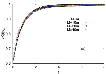
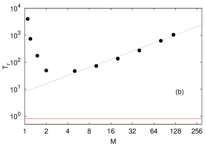
Figure 7: (a) $\langle\mathcal{K}(t)\rangle_{e}$ vs time for HD with different impurity mass values including $M=m$ (i.e. absence of the colloid). All curves collapse confirming that in the case of disks the relaxation time is independent of the presence of the colloid. The black curve represents the fit (17). (b) Relaxation time $\mathcal{T}_{r}$ vs $M$ needed for HPS to relax from a uniform to the Gaussian equilibrium distribution at $T=50$. Other parameters are fixed as in Fig. 3. The dotted straight line suggests a compatibility with a linear behavior at large mass ratios. The red horizontal line indicates $\mathcal{T}_{r}$ for the HD, which is put here for comparison and to show the independence of relaxation process on the presence of the colloid as already evidenced in (a).

The perfect collapse of the curves $\langle\mathcal{K}(t)\rangle_{e}$ for the HD system (Fig. 7a) obtained for four values of the ratio $M$ including the case $M=m=1$ (i.e. without the impurity), clearly indicates that the relaxation process of the disks is independent of the colloid. Unlike HD, for HPS the mass $M$ of the impurity is crucial in determining the relaxation. This is shown in Fig. 7b, where we report the behaviour of $\mathcal{T}_{r}$, fitted by using (17), as a function of $M$. As one can see, $\mathcal{T}_{r}$ diverges for $M\to m$ (identical squares) and $M\to\infty$ (immobile impurity which again does not allow for the exchange of energy, leading to the impossibility of relaxation). Notice that asymptotically $\mathcal{T}_{r}$ seems to grow linearly with $M$.

This results, although obvious when considering the different nature of the collisional processes occurring in the two systems, confirm that the relaxation to the equilibrium of HPS is much slower than that for HD and crucially depends on the impurity characteristics.

5 Final remarks

From the results presented in this paper we obtain good indications that a non-chaotic system with many degrees of freedom, consisting of a gas of hard squares, provides a suitable model for Brownian motion which is equivalent, at least at a simulation level, to the corresponding chaotic model, where squares are replaced by disks.

A deep understanding the role of chaos for Brownian motion and for transport properties is a very important issue deserving further comments. With reference to previous works, we now discuss this issue by stressing how the presence/absence of ergodicity, mixing and chaos in the microscopic dynamics (may) influence the statistical mechanics of macroscopic systems.

Let us start with a few remarks on equilibrium statistical mechanics, where the problem of connecting (micro)dynamics and (macro)statistical features is at the origin of Boltzmann’s ergodic hypothesis. First, it is worth noticing that ergodicity, in its strict mathematical formulation, is an extremely demanding property. Second, in spite of its theoretical importance, it is not completely satisfactory from a physical point of view as it involves global asymptotic limits, rarely encountered in practice. However, for the foundation of statistical mechanics, a widespread consensus exists on the key role played by the huge number of degrees of freedom involved in a macroscopic system rather than ergodicity. This point of view received mathematical support from the works by Khinchin [23], Mazur and van der Linden [24], and others. They proved that statistical mechanics works independently of ergodicity thanks to the existence of meaningful physical observables (the so-called sum functions) which are nearly constant on the energy surface, apart from regions of vanishing measure. Support to this picture comes from the results of Frisch and coworkers [28, 29, 30, 31], who found robust statistical phenomena in a trivially non-ergodic system. Nevertheless, Khinchin’s statements cannot be the ultimate grounding of statistical mechanics because not all physically important observables belong to the class of the sum functions.

Since chaos grants the validity of some “statistical laws” even in few degrees of freedom systems, one could be tempted to invoke it as the sufficient ingredient to build a robust statistical mechanical approach grounded on Hamiltonian systems. However, for this to be true, chaos in the microscopic dynamics should be enough “strong”. Indeed, results of extended simulations in high dimensional systems [46, 47, 48] have shown that chaos may be not enough to ensure the validity of the equilibrium statistical mechanics.

Let us now discuss this issue in the non-equilibrium statistical mechanics context, where the analogous of ergodicity is the mixing condition. As before, this condition is very demanding, being related to the $\Gamma$-space (the set of positions and momenta of system particles); while the study of macroscopic systems usually focuses on physical observable involving some projection procedures, amounting to neglect (or average) the effects of a large number of degrees of freedom in favor of few relevant variables. For instance, in the case of elementary transport properties the observable that matters refer to single particle properties: mean square particle displacement, correlation function and the response function either of the colloidal particle or the single gas particle. Therefore, one can wonder about the microscopic conditions ensuring a “good” statistical behavior for the above quantities.

We can start by considering few degrees of freedom systems, where also simple deterministic chaotic models may exhibit transport properties similar to those of more realistic systems. Paradigmatic examples are chaotic billiards and the Lorentz gas, where particle trajectories are chaotic as a consequence of the convexity of the obstacles. Numerical and theoretical works have shown that, in these systems (under appropriate hypothesis such as hyperbolicity etc.) the transport coefficients can be quantitatively related to chaos indicators [6, 7]. This would suggest that chaos is tightly related to transport. However, several examples of non-chaotic deterministic systems, such as a bouncing particle in a two-dimensional billiard with polygonal randomly distributed obstacles, possess robust transport properties [12, 13, 14, 16, 18]. For these non-chaotic models, it has been proposed that a sort of non-linear instability mechanism is required to observe diffusion [14]. The existence of non-chaotic models able to display diffusion poses some doubts on the possibility to make strong statements on the role of chaos for transport. It is however important to stress that in all these models the particles do not interact, and therefore, at least from a statistical mechanics point of view, they are rather artificial.

More interesting it is thus to consider many degrees of freedom systems, such a those investigated in this work. In this case the existence of quantitative relationships among chaos indicators and transport coefficients is, to the best we know, less clear (see for example [49, 50]). Nevertheless, chaos has been proved to be relevant in the establishment of some non-equilibrium properties [51]. Moreover, it is fair to say that diffusion of particles is rather common in chaotic many body particle systems. On the other hand, the non-chaotic model here investigated together with the previous results by Frisch and coworkers [28, 29, 30] indicate that transport properties for both impurity and gas particles agree with the prediction of kinetic theory and are indistinguishable from those of the (mixing) hard disk model. Therefore chaos, at least in the sense of positive Lyapunov exponents, cannot be invoked to explain the observed statistical behaviors. Nevertheless, as for low dimensional models [14], also in HPS a non infinitesimal mechanism of instability can be induced by the presence of singular corners of the squares, and these likely play a role for the diffusive behaviour.

We interpret these findings in the framework developed by Khinchin: the “good transport” properties observed in the non-mixing system result from the large number of particles and not from chaos. This is well evident for the correlation and response functions for the hard squares when, e.g., all particle are identical and the collision dynamics reduces to a mere relabelling. In such a case the exponential relaxation of $C_{v}(t)$ and $R_{v}(t)$ is just a probabilistic consequence of the exponential distribution of the time interval between two consecutive collisions. We stress that here diffusive properties are the outcome of the action of many degrees of freedom, and not of non-linear instability mechanisms as in low dimensional chaotic and non-chaotic models. Of course, as discussed in Sect. 4.2, chaos may favour the equilibration of the system.

As a last remark we note that the Gallavotti-Cohen [52] fluctuation theorem seems to apply to non-chaotic models, at least in finite time intervals, as shown by Benettin et al. [53] who investigated a non-equilibrium version of the Ehrenfest wind-tree model, which is non-chaotic. In such a system, although the maximum Lyapunov exponent is zero, the presence of long irregular transients, introduces an “effective randomness”.

In conclusion, we think that it is very difficult to decipher the signature of chaos in transport phenomena observed in many particles systems because, as shown in this paper, it can be overwhelmed by the emergence of an “effective dynamical randonmess” due to the combination of: a) coarse-graining procedure, b) finite scale instability and c) presence of a huge number of degrees of freedom. The characterization of this “effective randomness” requires the renounce to asymptotic limits (arbitrarily long time and arbitrary resolution) in favour of a finite time and/or finite resolution analysis [11, 12, 54, 55].

Appendix A Computation of the diffusion coefficient

In this Appendix, we detail the computation of the diffusion coefficient for the colloidal particle in an uniform and rarefied HD and HPS gas, following elementary kinetic theory. The basic idea is to estimate the average drag force exerted by the gas particles which collide with the impurity, by calculating the average exchanged momentum in the collisions.

Consider a rarefied HD gas at equilibrium, and focus on the collision of the colloidal disk characterized by its mass $M$, radius $R$ and precollisional velocity $\bm{V}$ with the gas particles which are characterized by $m,r,\bm{v}$, respectively. According to Eq. (2), the implulse transferred in the collision is

$$M{\bm{\Delta}}{\bm{V}}=M({\bm{V}}^{\prime}-{\bm{V}})=\frac{2mM}{m+M}{\bm{g}}\,,$$

${\bm{g}}={\bm{v}}-{\bm{V}}$ being the precollisional relative velocity. The rate of such collisions can be obtained by considering the equivalent problem of a colloid, at rest, with radius $r+R$, and hit by a flux of pointlike particles moving at relative velocity ${\bm{g}}$. The rate is then determined by counting the number of pointlike particles hitting the unit surface per unit time for a given orientation ${\bm{e}}$. This number corresponds to the particles contained in the collisional cylinder of infinitesimal base $(R+r)d\theta$ and height $\rho|{\bm{g}}\cdot{\bm{e}}|\Theta(-{\bm{e}}\cdot{\bm{g}})\delta t$, as shown in Fig. 8. The unitary step function $\Theta(s)$ selects the condition, $\bm{g}\cdot\bm{e}<0$, to have a collision.

Accordingly, the mean impulsive force in the normal direction ${\bm{e}}=\{\cos(\theta),\sin(\theta)\}$ selected by the $\theta$-angle that ${\bm{e}}$ forms with vector ${\bm{V}}$ (taken as $x$-axis direction)

$$\bigg{\langle}M\frac{\delta\bm{V}_{n}}{\delta t}\bigg{\rangle}=\frac{2mM}{m+M}\rho(R+r)\int_{0}^{2\pi}\!\!\!d\theta\int\!\!d{\bm{v}}P({\bm{v}})\Theta(-{\bm{e}}\cdot{\bm{g}})|{\bm{g}}\cdot{\bm{e}}|({\bm{g}}\cdot{\bm{e}}){\bm{e}}\,,\quad$$ (18)

the average is meant over the equilibrium distribution of the gas velocities $P(\bm{v})=m/(2\pi T)\exp[-m|{\bm{v}}|^{2}/(2T)]$. It is convenient to make the change of variable $(v_{x},v_{y})\to(g_{x},g_{y})$ and then perform the approximation $P({\bm{v}})\simeq P({\bm{g}})[1-m/T{\bm{g}}\cdot{\bm{V}}]$, justified in the limit $M\gg m$. After this manipulation, the integral (18) becomes

$$\bigg{\langle}M\frac{{\delta}{\bm{V}}_{n}}{\delta t}\bigg{\rangle}\simeq-\frac{4m^{2}M}{T(m+M)}\rho(R+r)\int_{0}^{2\pi}\!\!d\theta\!\int\!\!d{\bm{g}}P({\bm{g}})\Theta(-{\bm{e}}\cdot{\bm{g}})({\bm{g}}\cdot{\bm{e}})^{2}({\bm{g}}\cdot{\bm{V}})\,{\bm{e}}\;.\quad$$

This expression, recast in the form $M\dot{{\bm{V}}}=-\gamma M{\bm{V}}$, allows to explicitate the friction coefficient $\gamma$. Passing to polar coordinates, $g_{x}=g\cos(\alpha),g_{y}=g\sin(\alpha)$, simplifies the integral ($\alpha$ being the angle between ${\bm{g}}$ and ${\bm{V}}$, whose direction coincides with $x$-axis). Indicating by $\phi$ the angle between ${\bm{e}}$ and ${\bm{g}}$, we end up with

$$\int_{0}^{2\pi}d\theta\int_{0}^{\infty}dgP(g)g^{4}\int_{0}^{2\pi}d\alpha|\cos(\phi)|cos(\phi)\Theta[-\cos(\phi)]V\cos(\alpha)\,\cos(\theta)\;.$$

where the angles $\alpha,\theta,\phi$ are related by $\theta-\alpha=\pi-\phi$. The integration over $g$ yields $3/(2\pi)\sqrt{\pi/2}(m/T)^{-3/2}$, and that one on the angles gives the value $4\pi/3$. We then obtain the friction coefficient

$$\gamma=2\sqrt{2\pi}\,\frac{\rho R\sqrt{mT}}{M}\left(\frac{1+{r}/{R}}{1+{m}/{M}}\right)\,.$$ (19)

where the last factor takes into account finite size and mass corrections. By using Eq. (6) the diffusion constant is obtained as

$$D_{c}=\frac{T}{M\gamma}=\frac{1}{2\sqrt{2\pi}}\frac{1}{\rho R}\sqrt{\frac{T}{m}}\left(\frac{1+m/M}{1+r/R}\right)$$ (20)

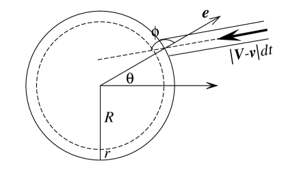
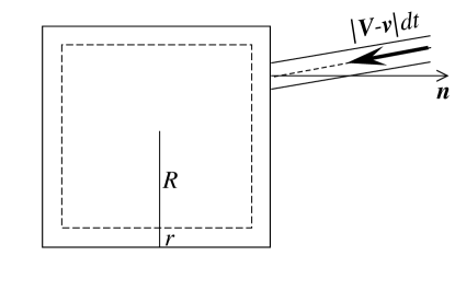
Figure 8: Cartoon of geometric construction used to compute the collision rate between an HD and HPS colloidal particle characterized by $(M,R,{\bm{V}})$, and gas particles $(m,r,{\bm{v}})$. The equivalent problem considers the colloid at rest, but with increased size $R+r$, and pointlike gas particles moving at the relative velocity ${\bm{v}}-{\bm{V}}$. The collision rate amount counting the number of gas particles contained in the collisional cylinder.

The same computation can be repeated for HPS, the only difference lying in the geometry of the problem (Fig. 8). Thanks to the symmetry, it is convenient to decompose the average impulse transferred from the gas to the colloidal particle in the x and y components (along the directions $(1,0)$, or $(0,1)$). For example, in the x-direction we have

$$\bigg{\langle}M\frac{{\delta V}_{x}}{\delta t}\bigg{\rangle}\simeq-\frac{4m^{2}M}{T(m+M)}\rho(R+r)V_{x}\sum_{n_{x}=\pm 1}\int\!\!dg_{x}P(g_{x})\Theta(-g_{x}n_{x})(g_{x}n_{x})^{2}|g_{x}|$$

Notice that the sum over $n_{x}=\pm 1$ stems from the two identical contributions to the exchanged momentum given by the left and right collisions occurring on the opposite sides of the square. The integral can be solved in Cartesian coordinates, and considering that the constraint imposed by $\Theta[-g_{x}n_{x}]$ amounts to a factor $2$. We thus obtain

$$\bigg{\langle}M\frac{{\delta V}_{x}}{\delta t}\bigg{\rangle}=-\frac{8m^{2}M}{T(m+M)}\rho(R+r)V_{x}\int_{0}^{\infty}dg_{x}P(g_{x})g_{x}^{3}\;.$$

The integration gives the value $\sqrt{2/\pi}(m/T)^{3/2}$ yielding the final results for the friction coefficient

$$\gamma=8\sqrt{\frac{2}{\pi}}\frac{\sqrt{m}\rho R\sqrt{T}}{M}\left(\frac{1+{r}/{R}}{1+{m}/{M}}\right)\,,$$ (21)

and thus the diffusion coefficient reads

$$D_{c}=\frac{\sqrt{\pi}}{8\sqrt{2}}\frac{1}{\rho R}\sqrt{\frac{T}{m}}\left(\frac{1+m/M}{1+r/R}\right)\,.$$ (22)

References

References

- [1] Einstein A, Ueber die von der molekularkinetischen Theorie der Waerme geforderte Bewegung von in ruhenden Fluessigkeiten suspendierten Teilchen, 1905 Ann. Phys. 17 549
- [2] Smoluchowski M, Zur kinetischen Theorie der Brownschen Molekularbewegung und der Suspensionen, 1906 Ann. Phys. 21 756
- [3] Geisel T and Nierwetberg J, Onset of Diffusion and Universal Scaling in Chaotic Systems, 1982 Phys. Rev. Lett. 48 7
- [4] Grossmann S and Fujisaka H, Diffusion in discrete nonlinear dynamical systems, 1982 Phys. Rev. A 26 1779
- [5] Klages R and Dorfman J R, Simple maps with fractal diffusion coefficients, 1995 Phys. Rev. Lett. 74 387
- [6] Gaspard P and Nicolis G, Transport properties, Lyapunov exponents, and entropy per unit time, 1990 Phys. Rev. Lett. 65 1693
- [7] Viscardy S and Gaspard P, Viscosity in the escape-rate formalism, 2003 Phys. Rev. E 68 041205
- [8] Gaspard P and Dorfman J R, Chaotic scattering theory, thermodynamic formalism, and transport coefficients, 1995 Phys. Rev. E 52 3525
- [9] Dorfman J R An Introduction to Chaos in Nonequilibrium Statistical Mechanics, 1999 (Cambridge: Cambridge University Press)
- [10] Gaspard P, Chaos, scattering and statistical mechanics, 1998 (Cambridge: Cambridge University Press)
- [11] Vega J L, Uzer T, Borondo F and Ford J, Deterministic diffusion in almost integrable systems 1996 Chaos 6 519
- [12] Dettmann C P and Cohen E D G, Microscopic chaos and diffusion, 2000 J. Stat. Phys. 101 775
- [13] Dettmann C P and Cohen E D G, Note on chaos and diffusion, 2001 J. Stat. Phys. 103 589
- [14] Cecconi F, del-Castillo-Negrete D, Falcioni M and Vulpiani A, The origin of diffusion: the case of non-chaotic systems, 2003 Physica D 180 129; Cecconi F, Cencini M, Falcioni M and Vulpiani A, Brownian motion and diffusion: from stochastic processes to chaos and beyond 2005 Chaos 15 026102
- [15] Lepri S, Livi R and Politi A, Thermal conduction in classical low-dimensional lattices, 2003 Phys. Rep. 377 1
- [16] Alonso D, Artuso R, Casati G and Guarneri I, Heat conductivity and dynamical instability, 1999 Phys. Rev. Lett. 82 1859
- [17] Li B, Casati G and Wang J, Heat conductivity in linear mixing systems, 2003 Phys. Rev. E 67 021204
- [18] Li B, Wang L and Hu B, Finite Thermal Conductivity in 1D Models Having Zero Lyapunov Exponents, 2002 Phys. Rev. Lett. 88 223901
- [19] Grassberger P, Nadler W and Yang L, Heat conduction and entropy production in a one-dimensional hard-particle gas, 2002 Phys. Rev. Lett. 89 180601
- [20] Cecconi F, Livi R and Politi A, Fuzzy transition region in a 1D coupled-stable-map lattice 1998 Phys. Rev. E 57 2703
- [21] Gaspard P., Comment on dynamical randomness in quantum systems 1994 Prog. Theor. Phys. Suppl. 116 369
- [22] Prigogine I and Stengers I, Entre le temps et l’éternité, 1979 (Paris: Fayards); Prigogine I, Laws of Nature, Probability and Time Symmetry Breaking, 1999 Physica A 263 528
- [23] Khinchin A I, Mathematical Foundations of Statistical Mechanics, 1949 (New York: Dover Publications Inc.)
- [24] Mazur P and van der Linden J, Asymptotic form of the structure function for real systems, 1963 J. Math. Phys. 4 271
- [25] Bricmont J, Science of chaos or chaos in science?, 1996 Ann. New York Ac. of Sciences 775 131
- [26] Holley R, Motion of a heavy particle in an infinite one dimensional gas of hard spheres, 1971 Zeit. Wahrsch. Verw. Geb. 17 181
- [27] Dürr D, Goldstein S and Lebowitz J L, A mechanical model of Brownian motion, 1981 Comm. Math. Phys. 78 507
- [28] Szu H H, Bdzil J, Carlier C, and Frisch H L, Molecular-dynamics verification of a final velocity distribution of a nonergodic system of hard parallel squares, 1974 Phys. Rev. A 9 1359
- [29] Frisch H L, Roth J, Krawchuk B D, and Sofinski P, Molecular dynamics of nonergodic hard parallel squares with a Maxwellian velocity distribution 1980 Phys. Rev. A 22 740
- [30] Carlier C and Frisch H L, Molecular Dynamics of Hard Parallel Squares 1972 Phys. Rev. A 6 1153; Molecular-Dynamics Study of Clustering in Hard Parallel Squares 1973 Phys. Rev. A 7 348
- [31] Rudd W G, and Frisch H L, The equation of state of parallel hard squares, 1971 J. Comp.Phys 7 394
- [32] Kubo R, Brownian motion and nonequilibrium statistical mechanics, 1986 Science 233 330
- [33] Kubo R, Toda M and Hashitsume N, Statistical Physics, vol 2. 1985 (Berlin: Springer-Verlag)
- [34] Grassia P, Dissipation, fluctuations and conservation laws, 2001 Am. J. Phys. 69 113
- [35] Allen M P and Tildesley T J, Computer simulation of Liquids, 1993 (Oxford: Clarendon Press)
- [36] Garcia-Rojo R, Luding S, and Brey J J, Transport coefficients for dense hard-disk systems, 2006 Phys. Rev. E 74 061305
- [37] Lorentz H A, The motion of electrons in metallic bodies, 1905 Proc. Amst. Acad. 7 438, 585, 684
- [38] van Beijeren H, Dorfman J R, Cohen E G D, Posch H A, and Dellago C, Lyapunov Exponents from Kinetic Theory for a Dilute, Field-Driven Lorentz Gas, 1996 Phys. Rev. Lett. 77 1974
- [39] Alder B J and Wainwright T E, Decay of the Velocity Autocorrelation Function, 1967 Phys. Rev. Lett. 18 988
- [40] Dorfman J R and Cohen E G D, Velocity Correlation Functions in Two and Three Dimensions 1970 Phys. Rev. Lett. 25 1257
- [41] Perondi L F and Binder P M, Mean-squared displacement of a hard-core tracer in a periodic lattice, 1993 Phys. Rev. B 48 4136
- [42] Chernov N and Lebowitz J L, Dynamics of a Massive Piston in an Ideal Gas: Oscillatory Motion and Approach to Equilibrium, 2002 J. Stat. Phys. 109 507
- [43] Ackland G J, Equipartition and ergodicity in closed one-dimensional systems of hard spheres with different masses, 1993 Phys. Rev. E 47 3268
- [44] Shirts R B, Burt S R and Johnson A M, Periodic boundary condition induced breakdown of the equipartition principle and other kinetic effects of finite sample size in classical hard-sphere molecular dynamics simulation, 2006 J. Chem. Phys. 125 164102
- [45] Chirikov B V, Universal instability of many-dimensional oscillator systems, 1979 Phys. Rep. 52 263
- [46] Livi R, Pettini M, Ruffo S and Vulpiani A, Chaotic behaviour in nonlinear Hamiltonian systems and equilibrium statistical mechanics, 1987 J. Stat. Phys. 48 539
- [47] Benettin G, Galgani L, Giorgilli A, Boltzmann ultraviolet cutoff and Nekhoroshev theorem on Arnold diffusion 1984 Nature 311 444
- [48] Alabiso C, Casartelli M, Marenzoni P, Thermodynamic limit beyond the stochasticity threshold in nonlinear chains, 1993 Phys. Lett. A 183 305
- [49] Barnett D M, Tajima T, Nishihara K, Ueshima Y, and Furukawa H, Lyapunov Exponent of a Many Body System and Its Transport Coefficients, 1996 Phys. Rev. Lett. 76 1812
- [50] Torcini A, Dellago C and Posch H A, comment on “Lyapunov exponent of a many body system and its transport coefficients 1999 Phys. Rev. Lett 83 2676
- [51] Evans D J, Cohen E G D and Morriss G P, Viscosity of a simple fluid from its maximal Lyapunov exponents, 1990 Phys. Rev. A 42 5990; Sarman S, Evans D J and Morriss G P, Conjugate-pairing rule and thermal-transport coefficients, 1992 Phys. Rev. A 45 2233
- [52] Gallavotti G and Cohen E G D, Dynamical Ensembles in Nonequilibrium Statistical Mechanics, 1995 Phys. Rev. Lett. 74 2694
- [53] Lepri S, Rondoni L and Benettin G, The Gallavotti–Cohen Fluctuation Theorem for a Nonchaotic Model, 2000 J. Stat. Phys. 99 857
- [54] Gaspard P and Wang X J, Noise, chaos and -entropy per unit time, 1993 Phys. Reports 235 291
- [55] Boffetta G, Cencini M, Falcioni M and Vulpiani A, Predictability: a way to characterize complexity, 2002 Phys. Reports 356 367