Inflation in a refined racetrack

Abstract

In this note, we refine the racetrack inflation model constructed in [3] by including the open string modulus. This modulus encodes the embedding of our braneworld inside some Calabi-Yau throat. We argue that in generic this open string modulus dynamically runs with the inflaton field thanks to its nonlinear coupling. A full analysis becomes difficult because the scalar potential changes progressively during the inflation epoch. Nevertheless, by explicit construction we are still able to build a realistic model through appropriate choices of the initial conditions.

1 Introduction and summary

Several inflation models motivated by string theory have been investigated so far[1, 2, 3, 4]. Provided enormous landscape of vacua via various scenarios of string compactification[5], they are equally interesting for the reason that our universe might happen to be described by one of them or a combination of some. String models of slow-roll inflation fall into two major categories: In the scenario of brane inlfation, the inflaton field is identified with the location of a mobile D3-brane in a warped throat of the compactified manifold, while in the scenario of moduli inflation the role of inflaton field is played by one or more string moduli. In particular, as a simple example to the latter category, an inflation model was developed using a racetrack potential inspired by KKLT construction[2] within the context of type IIB string theory[3], and later refined by an explicit construction[6] of specific orbifolded Calabi-Yau manifold with two Kähler moduli[4]. One feature of this type of inflation model is that the nonperturbative part of superpotential has a form of double exponentials. With appropriate choices of the parameters, this model can give rise to the desired slow-roll inflation, which seems difficult to achieve in the original KKLT model with single exponential. Though both racetrack models gave reasonable results consistent with the observational data, some underlying assumptions may still be questionable. One of them is the assumption that all the moduli are fixed priorly except for some specific Kähler modulus, which acts as the inflaton field. This assumption may not be generically justified if some moduli are coupled to each other too strongly to be integrated out separately. In this note, we would like to slightly relax the above-mentioned assumption by allowing one open string modulus, which encodes the embedding of our braneworld inside the Calabi-Yau throat, freely run with the inflaton field. We will only restrict our discussion based on the original racetrack model[3] since the functional dependence of open string modulus in the superpotential has been known[7, 8]. At the end, we find that this modulus in generic takes nonzero expectation value and therefore the racetrack potential would never be the same as that in [3]. We have found our braneworld is energetically pushed away from the tip of throat and the open string modulus is settled at some nonzero value. Our result could still be trusted even if deformation is applied to the conifold singularity of tip, as long as deforming parameter is small enough compared to the open string modulus. Moreover, contribution from this modulus increases with the e-folding so that it cannot be simply ignored during the period of inflation. A full analysis becomes difficult because the scalar potential changes progressively during the inflation epoch. Nevertheless by explicit construction through appropriate choices of the initial conditions in the moduli space, we are still able to build a realistic model achieving enough e-foldings and consistent with the present day observation.

This paper is organized in the following way. First we briefly review the original racetrack inflation model in the section 2. In the section 3, we introduce the open string modulus and derive the effective potential and discuss its vacua configuration. Then in the section 4, with appropriate choices of parameters and initial conditions, we explicitly build a realistic racetrack model which satisfies the slow-roll condition. Some derivation of useful formula are given in the Appendix. In this note, we have set Newton constant $G$ and Plank mass $M_{pl}$ to $1$ for convenience.

We remark that different modification of racetrack inflation was also discussed recently in [9, 10].

2 Brief review on racetrack inflation

We begin with a brief review on derivation of racetrack potential from the KKLT construction. We consider a compactification of ten-dimensional type IIB string theory on Calabi-Yau manifold with throats in the presence of three-form RR and NSNS fluxes $H_{(3)}$[11] and some stacks of D7-branes or Euclidean D3-branes wrapping around four-cycles of the compact space[2]. These background fluxes generate appropriate potentials which fix the values of type IIB axion-dilaton field and all the complex and Kähler moduli of Calabi-Yau space except one, denoted as $T=X+iY$. We may think of $X$ as the volume of compactified space and $Y$ as the axion field. Our world may be seated on a stack of D3-branes inside one of the throats. Now we consider a modified racetrack superpotential inspired by KKLT,

$$W=W_{0}+A_{1}e^{-a_{1}T}+A_{2}e^{-a_{2}T}.$$ (1)

The constant term is obtained through $W_{0}=\int{H_{(3)}\wedge\Omega}$ for the Calabi-Yau three form $\Omega$. The exponential terms are obtained through gaugino condensation nonperturbatively in a theory with a product gauge group, in our case $SU(N_{1})\times SU(N_{2})$. Coefficient $a_{i}=2\pi/N_{i}$ and $N_{i}$ is the number of coincident D7 branes in each stack. Coefficient $A_{i}$’s come from the fact that gauge coupling is proportional to the volume of compactified manifold and the latter is warped by the presence of branes. They were fixed in the original racetrack model but we will argue at this point in the next section. Following KKLT, the scalar potential induced on our braneworld composes of two parts

$$V=V_{F}+\delta V.$$ (2)

We recall that $V_{F}$ is the F-term potential for the $N=1$ effective four-dimensional theory, namely,

$$V_{F}=e^{K}(K^{i\bar{j}}D_{i}W\overline{D_{j}W}-3|W|^{2}),$$ (3)

provided that Kähler potential depends only on this Kähler modulus or equivalently the volume of Calabi-Yau space, namely

$$K=-3\ln{(T+\bar{T})}=-3\ln{2X}.$$ (4)

We remark that supersymmetric vacua should satisfy the following conditions,

$$D_{i}W=\partial_{i}W+\partial_{i}KW=0,$$ (5)

for each modulus, seen as a scalar field $\varphi_{i}$ in the four-dimensional spacetime. Then the scalar potential is either zero or negative, given by

$$V_{F}=-3e^{-K}|W|^{2},$$ (6)

corresponding to a flat or de Sitter spacetime. However, we are more interested in vacua with broken supersymetry. The supersymmetry breaking term $\delta V$ is induced by the presence of anti-D3 branes, which can be placed at the end of throat and stablized by the flux. Its contribution is positive definite and takes form as follows,

$$\delta V=\frac{E}{X^{2}}.$$ (7)

Since we ask modulus $T$ plays the role of inflaton field in the background of broken supersymmetry, it does not respect the condition (5). With appropriate choices of parameters, the authors in [3] found several vacua where a saddle point exists with two local minima nearby. The $55$ e-foldings is achieved when the inflaton field slowly rolls away from its saddle point and inflation is terminated when it is trapped in one of the minima.

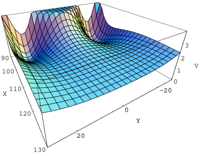
Figure 1: To the left, a snapshot of typical racetrack potential at local minimum of $\phi=1.79283\times 10^{-5}$. The potential has a saddle point at $X=123.16,Y=0$ and two nearby local minima. To the right, it shows the plot of potential given $X=123.16,Y=0$ in the vicinity of the local minimum $\phi=1.79283\times 10^{-5}$. The potential in both plots has been rescaled by $10^{16}$.

3 Effective potential and vacua configuration in the refined racetrack

In this section we would like to argue that the open string modulus, denoted as $\phi$, which was priorly dropped off in [3], may not be consistently integrated out at its supersymmetric vev thanks to the coupling with inflaton $T$ through the exponential terms. In this note, we may choose a local complex patch $\{z^{i}\}$ near the end of throat and $z\bar{z}=\phi$ is the embedding function of our braneworld inside the throat. The argument is as follows: as long as the volume of compactified manifold is changing during the inflation, the relative location between our braneworld and stacks of D7-branes are changing correspondingly. Therefore, it is reasonable to relax the assumption to allow modulus $\phi$ dynamically run with the Kähler modulus $T$. In a simplest situation such as the Ouyang embedding[12], D7-branes wrap around the holomorphic four-cycles parameterized by one complex parameter $\gamma_{i}^{-1}$. Then this open string modulus appears in the superpotential through $A_{i}$’s, namely[7, 8],

$$A_{i}(\phi)=\beta_{i}(1+\gamma_{i}\phi)^{1/N_{i}}.$$ (8)

Assuming that Kähler potential has additional dependence on the open string modulus $\phi$ as well as other messenger fields $f$ and $\tilde{f}$ (fundamental rep of gauge group on each stack of wrapped D7-branes.), such that a no-scale potential reads,

$$K=-3\ln{(T+\bar{T}-\phi\bar{\phi}-f\bar{f}-\tilde{f}\bar{\tilde{f}})}.$$ (9)

Now we propose a more general form for superpotential, namely,

$$W=W_{0}+A_{1}(\phi)e^{-a_{1}T}+A_{2}(\phi)e^{-a_{2}T}+m\phi f\tilde{f}.$$ (10)

In particular, applying condition (5), we obtain consistently truncated potential for $f=\tilde{f}=0$. However, the modulus $\phi$ fails to be simply integrated out provided the given superpotential and Kähler potential. To simplify the discussion, we will make a further assumption that the embedding only takes place in the real loci, i.e. both $\gamma_{i},\phi$ are real, though sometimes we still keep notation of $\bar{\phi}$. Then the scalar potential is again composed of two parts,

$$V=V_{F}(X,Y,\phi)+\delta V(X).$$ (11)

The effective potential $V_{F}$ contains two parts, whose explicit forms are given in the Appendix. We have denoted $V_{F}^{0}$(see equation (21)) as a reduction of full potential $V_{F}$ for $\phi=0$, which takes the same form as in [3]. However, the other component, denoted as $V_{F}^{1}$(see equation (22)), was not included in [3] and encodes most contribution of open string modulus to the full potential. We here also choose a specific setup suitable for racetrack inflation as found in [3] out of many other possibilities, say

$$\beta_{1}=\frac{1}{50},\qquad\beta_{2}=-\frac{35}{1000},\qquad a_{1}=\frac{2\pi}{100},\qquad a_{2}=\frac{2\pi}{90},$$

$$W_{0}=-\frac{1}{25000},\qquad E=4.14668\times 10^{-12}$$ (12)

with additional parameters of our choice,

$$\gamma_{1}=10^{-6},\gamma_{2}=-5.71429\times 10^{-7}.$$ (13)

This choice respects the relation $\gamma_{1}\beta_{1}=\gamma_{2}\beta_{2}$, which assures $D_{\phi}W=0$ at expectation value $\phi=0$ in case $N_{1}=N_{2}$, though there is no typical reason to do so in generic situation. For generic $N_{1}\neq N_{2}$, $\phi=0$ is only achievable via $X\to\infty$, meaning that this modulus is not stablized and the internal space becomes decompactified. We also remark that all the scaling symmetries as mentioned in [3], i.e. $\gamma$ and $\mu$-transformations, are broken for non-trivial dependence of $A_{i}$ on $\phi$. However, the discrete symmetry along $Y$ direction is still preserved, i.e. $Y\sim Y+nL(N_{1},N_{2})$ for integer $n$, where function $L(a,b)$ is the least common multiplier of two integers $a$ and $b$. With these chosen parameters, we have a saddle point at

$$X_{s}=123.216,\qquad Y_{s}=0,\qquad\phi_{s}=1.79283\times 10^{-5}.$$ (14)

and nearby minima locate at

$$X_{m}=93.7193,\qquad Y_{m}=\pm 23.1406,\qquad\phi_{m}=5.78999.$$

$$X_{m}=93.7193,\qquad Y_{m}=\pm 23.1407,\qquad\phi_{m}=-5.78999.$$ (15)

In the Figure 1, we plot the scalar potential at $\phi=\phi_{s}$. We remark several properties of this moduli space. First notice that $\phi\neq 0$ is expected in those specific locations, therefore the racetrack potential in [3] is not energetically favored in our refined model. During the inflation, we have found our braneworld, initially at $\phi=\phi_{s}$, is energetically pushed away from the tip of throat and settled at $\phi=\phi_{m}$ for the open string modulus. Our result could still be trusted even if deformation is applied to the conifold singularity of tip, as long as deforming parameter is small enough compared to $\phi_{s}$ and $\gamma_{i}^{-1}$.

Secondly, $V_{,yy}<0$ at the saddle point and one may guess that the initial motion of slow-roll is along Y-direction at least in case of no initial speed. We will see that this may not be true in our refined model.

At last, the contribution from $V_{F}^{1}$ becomes significant at large value of $\phi$; to see that we found $|V_{F}^{1}/V_{F}^{0}|$ varies from $10^{-11}$ to $0.28$ for inflaton moves from the saddle point to one of the minima, while $\delta V$ is about the same order as $V_{F}^{0}$. The saddle point implies a de Sitter space with $V\simeq 1.65489\times 10^{-16}$ and the minima are anti-de Sitter space with $V\simeq-1.148\times 10^{-16}$. Both have magnitude of order $10^{-16}$. If we increase $E$ up to $5.15815\times 10^{-12}$ or more in order to have Minkovski or de Sitter vacua at the minima, then the saddle point disappears and the slow-roll may not take place.

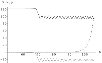
Figure 2: To the left, the plot shows each moduli evolves with e-folding $N$. The black solid line stands for modulus $X$, gray solid line for $Y$ and dashed line for $\phi$. To the right, it shows the power spectrum of scalar density perturbation evaluated at different values of $N$. We remark that $P\simeq 4\times 10^{-10}$ at $N=55$.

4 Slow-roll inlfation

In this section, we would like to discuss the condition for slow-roll inflation. We recall that the kinetic term of scalar fields are given in term of the Kähler potential (see equation (Appendix)), that is,

$${\cal L}_{kin} =\frac{1}{2}{\cal G}_{ij}\partial_{\mu}\varphi^{i}\partial^{\mu}\varphi^{j}$$ (16)

$$=\frac{3}{\Delta^{2}}(\partial_{\mu}X\partial^{\mu}X+\partial_{\mu}Y\partial^{\mu}Y)+\frac{6(\Delta-X)}{\Delta^{2}}\partial_{\mu}\phi\partial^{\mu}\phi.$$

For scalar fields having non-canonical kinetic terms, we have slow-roll parameters in general forms,

$$\epsilon=\frac{1}{2}(\frac{g^{ij}V_{,i}V_{,j}}{V^{2}}),$$

$$N^{i}{}_{j}=[\frac{g^{ik}(V_{,kj}-\Gamma^{l}_{kj}V_{,l})}{V}],$$ (17)

where $\eta$ is defined as the most negative eigenvalue of the matrix $N^{i}{}_{j}$. At the saddle point, $\epsilon$ is trivially zero and $\eta=-0.0384854$ for parameters of our choice.

The evolution of scalar fields is govern by the following equations of motion,

$$\ddot{\varphi^{i}}+3H\dot{\varphi^{i}}+\Gamma^{i}_{jk}\dot{\varphi^{j}}\dot{\varphi^{k}}+g^{ij}\frac{\partial V}{\partial\varphi^{j}}=0,$$

$$3H^{2}=\frac{1}{2}{\cal G}_{ij}\dot{\varphi^{i}}\dot{\varphi^{j}}+V,$$ (18)

where the Hubble constant $H\equiv\dot{a}/a$. We have listed equations of motion for each scalar $\varphi^{i}=X,Y,\phi$ in the Appendix. The term linear to $\dot{\varphi}$ plays the role of friction, while the gradient of potential gives rise to the conservative force. We remark that the nontrivial Levi-Civita connections defined on the moduli space encode the complicate couplings among those scalars fields and we have them listed in the Appendix too.

Assuming that inflation starts at rest at the saddle point, we find that before inflation ends at $\epsilon=1$, we only have about $47$ e-foldings, which is too small for our observational universe. However, with fine-tuned initial speed $X_{s}^{\prime}=-0.02$, we are able to achieve in total about $106$ e-foldings, as shown in the Figure 2. We also have power spectrum of scalar density perturbation $P(k)\simeq 4\times 10^{-10}$ at $55$ e-foldings, qualifying the COBE normalization. Provided $\epsilon=2.80795\times 10^{-10}$ and $\eta=-0.0235525$ at the $55$ e-foldings, one obtains the spectral index,

$$n(k)\simeq 1-6\epsilon+2\eta=0.952895,$$ (19)

which agrees well with the observational data. We remark that the initial motion of inflaton field with zero initial speed is in fact along $\phi$-direction, instead of $Y$-direction as observed in [3]. The inflaton field with $X^{\prime}_{s}\neq 0$ makes additional detour along $X$-direction. We plot both cases in the Figure 3 for the first few e-foldings.

We argue that there seems no criteria to assign any particular initial condition for inflaton fields, provided no sound knowledge of probability measure in the moduli phase space. Therefore there seems no objection to assign some initial speed for inflaton fields as we just did. It might stand a good chance to find another set of parameters with inflaton fields of zero initial speed and achieving enough e-foldings, but that could be an exhausting search without some clever guiding principles. We will leave this issue for further study.

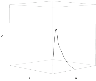
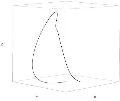
Figure 3: To the left, inflaton starts at rest, first moves towards $\phi$-direction and then $Y$-direction. To the right, infaton with initial speed $X^{\prime}_{s}=-0.02$ first makes additional detour along $X$-direction. The typical scale of each axis $X,Y,\phi$ is about $0.01,0.01$, and $10^{-9}$.

Appendix

Here we have listed the explicit forms of scalar potential and equations of motion. First a collection of useful formula for Kähler metrics and derivatives,

$$K_{T\bar{T}}=\frac{1}{2}{\cal G}_{XX}=\frac{1}{2}{\cal G}_{YY}=\frac{3}{\Delta^{2}},\qquad K_{\phi\bar{\phi}}=\frac{1}{2}{\cal G}_{\phi\phi}=\frac{6(\Delta-X)}{\Delta}$$

$$D_{T}W=-a_{1}A_{1}e^{-a_{1}T}-a_{2}A_{2}e^{-a_{2}T}-\frac{3}{\Delta}W,$$

$$D_{\phi}W=A_{i}^{\prime}e^{-a_{1}T}+A_{2}^{\prime}e^{-a_{2}T}+\frac{3\bar{\phi}}{\Delta}W,$$

$$\Delta=2X-|\phi|^{2},\qquad.$$ (20)

The scalar potential then reads,

$$V = V^{0}_{F}+V^{1}_{F}+\delta V,$$

$$V^{0}_{F} = \frac{1}{3\Delta}\biggl{[}a_{1}(a_{1}+\frac{6}{\Delta})A_{1}^{2}e^{-2a_{1}X}+a_{2}(a_{2}+\frac{6}{\Delta})A_{2}^{2}e^{-2a_{2}X}$$ (21)

$$+(a_{1}a_{2}+\frac{3}{\Delta}a_{1}+\frac{3}{\Delta}a_{2})A_{1}A_{2}e^{-(a_{1}+a_{2})X}2\cos{(a_{1}-a_{2})Y}$$

$$+\frac{3}{\Delta}a_{1}W_{0}A_{1}e^{-a_{1}X}2\cos{a_{1}Y}+\frac{3}{\Delta}a_{2}W_{0}A_{2}e^{-a_{2}X}2\cos{a_{2}Y}\biggr{]}$$

$$V^{1}_{F} = \frac{1}{6\Delta(\Delta-X)}\biggl{[}A_{1}^{\prime 2}e^{-2a_{1}X}+A_{2}^{\prime 2}e^{-2a_{2}X}+\frac{9|\phi|^{2}}{\Delta^{2}}|W|^{2}$$ (22)

$$+A_{1}^{\prime}A_{2}^{\prime}e^{-(a_{1}+a_{2})X}2\cos{(a_{1}-a_{2})Y}+\frac{3}{\Delta}(A_{1}^{\prime}\square_{1}+A_{2}^{\prime}\square_{2})\biggr{]},$$

$$\delta V = \frac{E}{X^{2}},$$ (24)

$$\square_{i}=-2\phi e^{-a_{i}X}(W_{1}\cos{a_{i}Y}+W_{2}\sin{a_{i}Y}),$$

where $T=X+iY$ and $W=W_{1}+iW_{2}$.

The nontrivial Levi-Civita connections in the moduli space are given as follows:

$$\Gamma^{X}_{XX}=-\Gamma^{X}_{YY}=-\frac{2}{\Delta},\qquad\Gamma^{X}_{\phi\phi}=\frac{\Delta-2\phi^{2}}{\Delta},\qquad\Gamma^{X}_{X\phi}=\frac{2\phi}{\Delta},$$

$$\Gamma^{Y}_{XY}=-\frac{2}{\Delta},\qquad\Gamma^{Y}_{Y\phi}=\frac{2\phi}{\Delta},$$ (25)

$$\Gamma^{\phi}_{\phi\phi}=-\frac{|\phi|^{2}\phi}{\Delta(\Delta-X)},\qquad\Gamma^{\phi}_{XX}=-\frac{\phi}{\Delta(\Delta-X)},$$

$$\Gamma^{\phi}_{X\phi}=\frac{2|\phi|^{2}-\Delta}{2\Delta(\Delta-X)},\qquad\Gamma^{\phi}_{YY}=\frac{\phi}{\Delta(\Delta-X)}.$$

Applying the equation (4) for each scalar fields, we have equations of motion

$$X^{\prime\prime}=-\Omega(3X^{\prime}+\frac{\Delta^{2}}{2}\frac{V_{,X}}{V})+\frac{1}{\Delta}(2X^{\prime 2}-2Y^{\prime 2}-(\Delta-2\phi^{2})\phi^{\prime 2}-4\phi X^{\prime}\phi^{\prime})$$

$$Y^{\prime\prime}=-\Omega(3Y^{\prime}+\frac{\Delta^{2}}{2}\frac{V_{,Y}}{V})+\frac{4}{\Delta}(X^{\prime}Y^{\prime}-\phi\phi^{\prime}Y^{\prime})$$

$$\phi^{\prime\prime}=-\Omega(3\phi^{\prime}+\frac{\Delta^{2}}{4(\Delta-X)}\frac{V_{,\phi}}{V})+\frac{1}{\Delta(\Delta-X)}[\phi(X^{\prime 2}+Y^{\prime 2})+\phi^{3}\phi^{\prime 2}+(\Delta-2\phi^{2})X^{\prime}\phi^{\prime}],$$

$$\Omega=1-\frac{X^{\prime 2}+Y^{\prime 2}+2(\Delta-X)\phi^{\prime 2}}{\Delta^{2}}.$$ (26)

References

References

- [1] G. R. Dvali and S. H. H. Tye, Phys. Lett. B 450, 72 (1999) [arXiv:hep-ph/9812483]. C. P. Burgess, M. Majumdar, D. Nolte, F. Quevedo, G. Rajesh and R. J. Zhang, JHEP 0107, 047 (2001) [arXiv:hep-th/0105204]. G. R. Dvali, Q. Shafi and S. Solganik, arXiv:hep-th/0105203. J. Garcia-Bellido, R. Rabadan and F. Zamora, JHEP 0201, 036 (2002) [arXiv:hep-th/0112147]. N. T. Jones, H. Stoica and S. H. H. Tye, JHEP 0207, 051 (2002) [arXiv:hep-th/0203163]. M. Gomez-Reino and I. Zavala, JHEP 0209, 020 (2002) [arXiv:hep-th/0207278]. C. P. Burgess, J. M. Cline, H. Stoica and F. Quevedo, JHEP 0409, 033 (2004) [arXiv:hep-th/0403119]. J. M. Cline and H. Stoica, Phys. Rev. D 72, 126004 (2005) [arXiv:hep-th/0508029]. J. P. Hsu, R. Kallosh and S. Prokushkin, JCAP 0312, 009 (2003) [arXiv:hep-th/0311077]. F. Koyama, Y. Tachikawa and T. Watari, Phys. Rev. D 69, 106001 (2004) [Erratum-ibid. D 70, 129907 (2004)] [arXiv:hep-th/0311191]. H. Firouzjahi and S. H. H. Tye, Phys. Lett. B 584, 147 (2004) [arXiv:hep-th/0312020]. J. P. Hsu and R. Kallosh, JHEP 0404, 042 (2004) [arXiv:hep-th/0402047]. E. Silverstein and D. Tong, Phys. Rev. D 70, 103505 (2004) [arXiv:hep-th/0310221]. R. Kallosh and S. Prokushkin, arXiv:hep-th/0403060. M. Alishahiha, E. Silverstein and D. Tong, Phys. Rev. D 70, 123505 (2004) [arXiv:hep-th/0404084]. X. Chen, JHEP 0508, 045 (2005) [arXiv:hep-th/0501184]. X. Chen, Phys. Rev. D 72, 123518 (2005) [arXiv:astro-ph/0507053]. D. Cremades, F. Quevedo and A. Sinha, JHEP 0510, 106 (2005) [arXiv:hep-th/0505252]. C. P. Burgess, P. Martineau, F. Quevedo, G. Rajesh and R. J. Zhang, JHEP 0203, 052 (2002) [arXiv:hep-th/0111025]. Z. Lalak, G. G. Ross and S. Sarkar, Nucl. Phys. B 766, 1 (2007) [arXiv:hep-th/0503178]. J. P. Conlon and F. Quevedo, JHEP 0601, 146 (2006) [arXiv:hep-th/0509012]. O. DeWolfe, S. Kachru and H. L. Verlinde, JHEP 0405, 017 (2004) [arXiv:hep-th/0403123]. N. Iizuka and S. P. Trivedi, Phys. Rev. D 70, 043519 (2004) [arXiv:hep-th/0403203].
- [2] S. Kachru, R. Kallosh, A. Linde and S. P. Trivedi, Phys. Rev. D 68, 046005 (2003) [arXiv:hep-th/0301240]. S. Kachru, R. Kallosh, A. Linde, J. M. Maldacena, L. P. McAllister and S. P. Trivedi, JCAP 0310, 013 (2003) [arXiv:hep-th/0308055].
- [3] J. J. Blanco-Pillado et al., JHEP 0411, 063 (2004) [arXiv:hep-th/0406230].
- [4] J. J. Blanco-Pillado et al., JHEP 0609, 002 (2006) [arXiv:hep-th/0603129].
- [5] F. Denef and M. R. Douglas, JHEP 0405, 072 (2004) [arXiv:hep-th/0404116]. F. Denef and M. R. Douglas, JHEP 0503, 061 (2005) [arXiv:hep-th/0411183]. B. S. Acharya, F. Denef and R. Valandro, JHEP 0506, 056 (2005) [arXiv:hep-th/0502060].
- [6] F. Denef, M. R. Douglas and B. Florea, JHEP 0406, 034 (2004) [arXiv:hep-th/0404257].
- [7] D. Baumann, A. Dymarsky, I. R. Klebanov, J. M. Maldacena, L. P. McAllister and A. Murugan, JHEP 0611, 031 (2006) [arXiv:hep-th/0607050].
- [8] O. DeWolfe, L. McAllister, G. Shiu and B. Underwood, JHEP 0709, 121 (2007) [arXiv:hep-th/0703088].
- [9] S. P. de Alwis, Phys. Rev. D 76, 086001 (2007) [arXiv:hep-th/0703247].
- [10] P. Brax, A. C. Davis, S. C. Davis, R. Jeannerot and M. Postma, arXiv:0710.4876 [hep-th].
- [11] S. B. Giddings, S. Kachru and J. Polchinski, Phys. Rev. D 66, 106006 (2002) [arXiv:hep-th/0105097].
- [12] P. Ouyang, Nucl. Phys. B 699, 207 (2004) [arXiv:hep-th/0311084].