Sequential Tracking of a Hidden Markov Chain Using Point Process Observations

Abstract.

We study finite horizon optimal switching problems for hidden Markov chain models with point process observations. The controller possesses a finite range of strategies and attempts to track the state of the unobserved state variable using Bayesian updates over the discrete observations. Such a model has applications in economic policy making, staffing under variable demand levels and generalized Poisson disorder problems. We show regularity of the value function and explicitly characterize an optimal strategy. We also provide an efficient numerical scheme and illustrate our results with several computational examples.

1. Introduction

An economic agent (henceforth the controller) observes a compound Poisson process $X$ with arrival rate $\lambda$, and mark/jump distribution $\nu$. The local characteristics $(\lambda,\nu)$ of $X$ are determined by the current state of an unobservable Markov jump process $M$ with finite state space $E\triangleq\{1,\ldots,m\}$. More precisely, the characteristics are $(\lambda_{i},\nu_{i})$ whenever $M$ is at state $i$, for $i\in E$.

The objective of the controller is to track the state of $M$ given the information in $X$. To do so, the controller possesses a range of policies $a$ in the finite alphabet $\mathcal{A}\triangleq\{1,\ldots,A\}$. The policies are sequentially adopted starting from time 0 and until some fixed horizon $T<\infty$. The infinite horizon case $T=+\infty$ is treated in Section 5.1. The selected policy $a$ leads to running costs (benefits) at instantaneous rate

$$\sum_{i\in E}c_{i}(a)1_{\{M_{t}=i\}}dt.$$

The controller’s overall strategy consists of a double sequence $(\tau_{k},\xi_{k}),k=0,1,2,\ldots$, with $\xi_{k}\in\mathcal{A}$ representing the sequence of chosen policies and $0\triangleq\tau_{0}<\tau_{1}<\dots\leq T$ representing the times of policy changes (from now on termed switching times). We denote the entire strategy by the right-continuous piecewise constant process $\xi\colon[0,T]\times\Omega\to\mathcal{A}$, with $\xi_{t}=\xi_{k}$ if $\tau_{k}\leqslant t<\tau_{k+1}$ or

(1.1) $$\xi_{t}=\sum_{\tau_{k+1}\leq T}\xi_{k}\cdot 1_{[\tau_{k},\tau_{k+1})}(t).$$

Beyond running benefits, the controller also faces switching costs in changing her policy which lead to inertia and hysteresis. If at time $t$, the controller changes her policy from $a$ to $b$ and $M_{t}=i$ then an immediate cost $K_{i}(a,b)$ is incurred. The overall objective of the controller is to maximize the total present value of all tracking benefits minus the switching costs which is given by

$$\int_{0}^{T}\mathrm{e}^{-\rho t}\left(\sum_{i\in E}c_{i}(\xi_{t})1_{\{M_{t}=i\}}\right)\,dt-\sum_{k}\mathrm{e}^{-\rho\tau_{k}}\left(\sum_{i\in E}K_{i}(\xi_{\tau_{k}-},\xi_{\tau_{k}})\cdot 1_{\{M_{\tau_{k}}=i\}}\right),$$

where $\rho\geq 0$ is the discount factor.

Since $M$ is unobserved, the controller must carry out a filtering procedure. We postulate that she collects information about $M$ via a Bayesian framework. Let $\vec{\pi}=(\pi_{1},\ldots,\pi_{m})\triangleq\left(\mathbb{P}\{M_{0}=1\},\ldots,\mathbb{P}\{M_{0}=m\}\right)$ be the initial (prior) beliefs of the controller about $M$ and $\mathbb{P}^{\vec{\pi}}$ the corresponding conditional probability law. The controller starts with beliefs $\pi$, observes $X$, updates her beliefs and adjusts her policy accordingly. Because only $X$ is observable, the strategy $\xi$ should be determined by the information generated by $X$, namely each $\tau_{k}$ must be a stopping time of the filtration $\mathcal{F}^{X}$ of $X$. Similarly, the value of each $\xi_{k}$ is determined by the information $\mathcal{F}^{X}_{\tau_{k}}$ revealed by $X$ until $\tau_{k}$. These notions and the precise updating mechanism will be formalized in Section 2.3. We denote by $\mathcal{U}(T)$ the set of all such admissible strategies on a time interval $[0,T]$. Since strategies with infinitely many switches would have infinite costs, we exclude them from $\mathcal{U}(T)$.

Starting with initial policy $a\in\mathcal{A}$ and beliefs $\vec{\pi}$, the performance of a given policy $\xi\in\mathcal{U}(T)$ is

(1.2) $$J^{\xi}(T,\vec{\pi},a)\triangleq\mathbb{E}^{\vec{\pi},a}\left[\int_{0}^{T}\mathrm{e}^{-\rho t}\left(\sum_{i\in E}c_{i}(\xi_{t})1_{\{M_{t}=i\}}\right)dt-\sum_{k}\mathrm{e}^{-\rho\tau_{k}}\!\left(\sum_{i\in E}K_{i}(\xi_{k-1},\xi_{k})\cdot 1_{\{M_{\tau_{k}}=i\}}\right)\right].$$

The first argument in $J^{\xi}$ is the remaining time to maturity. The optimization problem is to compute

(1.3) $$U(T,\vec{\pi},a)\triangleq\sup_{\xi\in\mathcal{U}(T)}J^{\xi}(T,\vec{\pi},a),$$

and, if it exists, find an admissible strategy $\xi^{*}$ attaining this value. In this paper we solve (1.3), including giving a full characterization of an optimal control $\xi^{*}$ and a deterministic numerical method for computing $U$ to arbitrary level of precision. The solution will proceed in two steps: an initial filtering step and a second optimization step. The inference step is studied in Section 2, where we convert the optimal control problem with partial information (1.3) into an equivalent fully observed problem in terms of the a posteriori probability process $\vec{\Pi}$. The process $\vec{\Pi}$ summarizes the dynamic updating of controller’s beliefs about the Markov chain $M$ given her point process observations. The explicit dynamics of $\vec{\Pi}$ are derived in Proposition 2.2, so that the filtering step is completely solved. The main part of the paper then analyzes the resulting optimal switching problem (2.6) in Sections 3 and 4.

To our knowledge, the finite horizon partially observed switching control problem (which might be viewed as an impulse control problem in terms of $\xi$) defined in (1.3), has not been studied before. However, it is closely related to optimal stopping problems with partially observable Cox processes that have been extensively looked at starting with the Poisson Disorder problems, see e.g. Peskir and Shiryaev (2000, 2002); Bayraktar and Dayanik (2006); Bayraktar et al. (2006); Bayraktar and Sezer (2006). In particular, Bayraktar and Sezer (2006) solved the Poisson disorder problem when the change time has phase type prior distribution by showing that it is equivalent to an optimal stopping problem for a hidden Markov process (which has several transient states and one absorbing state) that is indirectly observed through a point process. Later Ludkovski and Sezer (2007) solved a similar optimal stopping problem in which all the states of the hidden Markov chain are recurrent. Both of these works can be viewed as a special case of (1.3), see Remark 3.2. Our model can also be viewed as the continuous-time counterpart of discrete-time sequential $M$-ary detection in hidden Markov models, a topic extensively studied in sequential analysis, see e.g. Tartakovsky et al. (2006); Aggoun (2003).

Filtering problems with point process observations is a well-studied area; let us mention the work of Arjas et al. (1992), Ceci and Gerardi (1998) and the reference volume Elliott et al. (1995). In our model we use the previous results obtained in Bayraktar and Sezer (2006); Ludkovski and Sezer (2007) to derive an explicit filter; this allows us then to focus on the separated fully-observed optimal switching problem using the new hyper-state. Let us also mention the recent paper of Chopin and Varini (2007) who study a simulation-based method for filtering in a related model, but where an explicit filter is unavailable and must be numerically approximated.

The techniques that we use to solve the optimal switching/impulse control problem are different from the ones used in the continuous-time optimal control problems mentioned above. The main tool in solving the optimal stopping problems (in the multi-dimensional case, the tools in the one dimensional case are not restricted to the one described here) is the approximating sequence that is constructed by restricting the time horizon to be less than the time of the $n$-th observation/jump of the observed point process. This sequence converges to the value function uniformly and exponentially fast. However, in the impulse control problem, the corresponding approximating sequence is constructed by restricting the sum of the number of jumps and interventions to be less than $n$. This sequence converges to the value function, however the uniform convergence in both $T$ and $\vec{\pi}$ is not identifiable using the same techniques.

As in Costa and Davis (1989) and Costa and Raymundo (2000) (also see Mazziotto et al. (1988) for general theory of impulse control of partially observed stochastic systems), we first characterize the value function $U$ as the smallest fixed point of two functional operators and obtain the aforementioned approximating sequence. Using one of these characterization results and the path properties of the a posteriori probability process we obtain one of our main contributions: the regularity of the value function $U$. We show that $U$ is convex in $\vec{\pi}$, Lipschitz in the same variable on the closure of its domain, and Lipschitz in the $T$ variable uniformly in $\vec{\pi}$. Our regularity analysis leads to the proof of the continuity of $U$ in both $T$ and $\vec{\pi}$ which in turn lets us explicitly describe an optimal strategy.

The other characterization of $U$ as a fixed point of the first jump operator is used to numerically implement the optimal solution and find the value function. In general, very little is known about numerics for continuous-time control of general hidden Markov models, and this implementation is another one of our contributions. We combine the explicit filtering equations together with special properties of piecewise deterministic processes (Davis, 1993) and the structure of general optimal switching problems to give a complete computational scheme. Our method relies only on deterministic optimization sub-problems and lets us avoid having to deal with first order quasi-variational inequalities with integral terms that appear in related stochastic control formulations (see remark 3.3 below). We illustrate our approach with several examples on a finite/infinite horizon and a hidden Markov chain with two or three states.

Our framework has wide-ranging applications in operations research, management science and applied probability. Specific cases are discussed in the next subsection. As these examples demonstrate, our approach leads to sensible policy advice in many scenarios. Most of the relevant applied literature treats discrete-time stationary problems, and our model can be seen as a finite-horizon, continuous-time generalization of these approaches.

The rest of the paper is organized as follows: In Section 1.1 we propose some applications of our modeling framework. In Section 2 we describe an equivalent fully observed problem in terms of the a posteriori probability process $\vec{\Pi}$. We also analyze the dynamics of $\vec{\Pi}$. In Section 3 we show that $U$ satisfies two different dynamic programming equations. The results of Section 3 along with the path description of $\vec{\Pi}$ allows us to study the regularity properties of $U$ and describe an optimal strategy in Section 4. Our model can be extended beyond (1.3), in particular to cover the case of infinite horizon and the case in which the costs are incurred at arrival times. The extensions are described in Section 5. Extensive numerical analysis of several illustrative examples is carried out in Section 6.

1.1. Applications

In this section we discuss case studies of our model and the relevant applied literature.

1.1.1. Cyclical Economic Policy Making

The economic business cycle is a basis of many policy making decisions. For instance, the country’s central bank attempts to match its monetary policy, so as to have low interest rates in periods of economic recession and high interest rates when the economy overheats. Similarly, individual firms will time their expenditures to coincide with boom times and will cut back on capital spending in unfavorable economy states. Finally, investors hope to invest in the bull market and stay on the sidelines during the bear market. In all these cases, the precise current economy state is never known. Instead, the agents collect information via economic events, surveys and news, and act based on their dynamic beliefs about the environment. Typically, such news consist of discrete events (e.g. earnings pre-announcements, geo-political news, economic polls) which cause instantaneous jumps in agents’ beliefs. Thus, it is natural to model the respective information structure by observations of a modulated compound Poisson process. Accordingly, let $M$ represent the current state of the economy and let the observation $X$ correspond to economic news. Inability to correctly identify $M$ will lead to (opportunity) costs $c_{M_{s}}(\xi_{s})$. Hence, one may take $\mathcal{A}=E$ and $c_{a}(a)=0,c_{a}(b)<0$. The strategy $\xi$ represents the set of possible actions of the agent. The switching costs of the form $K(\xi_{s},\xi_{s-})>0$ correspond to the costly influence of the Federal Reserve changing its interest rate policy, or to the transaction costs incurred by the investor who gets in/out of the market. Depending on the particular setting, one may study this problem both in finite- and infinite-horizon setting, and with or without discounting. For instance, a firm planning its capital budgeting expenses might have a fixed horizon of one year, while a central bank has infinite horizon but discounts future costs. A corresponding numerical example is presented in Section 6.2.

1.1.2. Matching Regime-Switching Demand Levels

Many customer-oriented businesses experience stochastically fluctuating demand. Thus, internet servers face heavy/light traffic; manufacturing managers observe cyclical demand levels; customer service centers have varying frequencies of calls. Such systems can be modeled in terms of a compound Poisson request process $X$ modulated by the partially known system state $M$. Here, $X$ serves the dual role of representing the actual demands and conveying information about $M$. The objective of the agent is to dynamically choose her strategy $\xi$, so as to track current demand level. For instance, an internet server receives asynchronous requests $Y_{\ell}$, $\ell=1,2,\ldots$ (corresponding to jumps of $X$) that take $c(Y_{\ell},\xi_{t})$ time units to fulfill. The rate of requests and their complexity distribution depend on $M$. In turn, the server manager can control how much processing power is devoted to the server: more processors cut down individual service times but lead to higher fixed overhead. Such a model effectively corresponds to a controlled $M(\lambda)/G/\infty$-queue, where the arrival rate $\lambda$ is $M$-modulated, and where the distribution of service times depends both on $M$ and the control $\xi$. A related computational example concerning a customer call center is treated in Section 6.3.

A concrete example that has been recently studied in the literature is the insurance premium problem. Insurance companies handle claims in exchange for policy premiums. A standard model asserts that claims $Y_{1},Y_{2},\ldots$ form a compound (time-inhomogeneous) Poisson process $X$. Suppose that the rate of claims is driven by some state variable $M$ that measures the current background risk (e.g. climate, health epidemics, etc.), with the latter being unobserved directly. In Aggoun (2003), such a model was studied (in discrete time) from the inference point of view, deriving the optimal filter for the insurance environment $M$ given the claim process. Assume now that the company can control its continuous premium rate $c^{2}(\xi_{t})$, as well as its deductible level $c^{1}(\xi_{t})$. High deductibles require lowering the premium rate, and are therefore only optimal in high-risk environments. Furthermore, changes to policy provisions (which has a finite expiration date $T$) are costly and should be undertaken infrequently. The overall objective is thus,

$$\sup_{\xi\in\mathcal{U}(T)}\mathbb{E}^{\vec{\pi},a}\left[-\sum_{j=1}^{N(T)}\mathrm{e}^{-\rho\sigma_{j}}(Y_{j}-c^{1}(\xi_{\sigma_{j}}))_{+}+\int_{0}^{T}c^{2}(\xi_{t})\,dt-\sum_{k}\mathrm{e}^{-\rho\tau_{k}}\left(\sum_{i\in E}K_{i}(\xi_{k-1},\xi_{k})\cdot 1_{\{M_{\tau_{k}}=i\}}\right)\right],$$

where $N$ is the counting process for the number of claims. The resulting cost structure, which is a variant of (1.3), is described in Section 5.2.

1.1.3. Security Monitoring

Classical models of security surveillance (radar, video cameras, communication network monitor) involve an unobserved system state $M$ representing current security (e.g. $E=\{0,1\}$, where $0$ corresponds to a ‘normal’ state and $1$ represents a security breach) and a signal $X$. The signal $X$ records discrete events, namely artifacts in the surveyed space (radar alarms, camera movement, etc.). Benign artifacts are possible, but the intensity $\lambda$ of $X$ increases when $M_{t}=1$. If the signal can be decomposed into further sub-types, then $X$ becomes a marked point process with marks $(Y_{\ell})$. The goal of the monitor is to correctly identify and respond to security breaches, while minimizing false alarms and untreated security violations. Classical formulations (Tartakovsky et al., 2006; Peskir and Shiryaev, 2000) only analyze optimality of the first detection. However, in most practical problems the detection is ongoing and discrete announcement costs require studying the entire (infinite) sequence of detection decisions. Accordingly, our optimal switching framework of (1.3) is more appropriate.

As a simplest case, the monitor can either declare the system to be sound $\xi_{t}=1$, or declare a state of alarm $\xi_{t}=2$. This produces $M$-dependent penalty costs at rate $\sum_{j\in E}c_{j}(\xi_{t})1_{\{M_{t}=j\}}dt$; also changing the monitor state is costly and leads to costs $K$. A typical security system is run on an infinite loop and one wishes to minimize total discounted costs, where the discounting parameter $\rho$ models the effective time-horizon of the controller (i.e. the trade-off between the myopically optimal announcement and long-run costs). Such an example is presented in Section 6.1.

1.1.4. Sequential Poisson Disorder Problems

Our model can also serve as a generalization of Poisson disorder problems, (Bayraktar et al., 2006; Peskir and Shiryaev, 2002). Consider a simple Poisson process $X$ whose intensity $\lambda$ sequentially alternates between $\lambda_{0}$ and $\lambda_{1}$. The goal of the observer is to correctly identify the current intensity; doing so produces a running reward at rate $c_{0}(\xi_{t})$ per unit time, otherwise a cost at rate $c_{1}(\xi_{t})$ is assessed, where $\xi$ is the control process. Whenever the observer changes her announcement, a fixed cost $K$ is charged in order to make sure that the agent does not vacillate. Letting $M$, $M_{t}\in\{0,1\}$ denote the intensity state, and $\lambda=\lambda_{M_{t}}$ this example yet again fits into the framework of (1.3). Obvious generalizations to multiple values of $\lambda$ and multiple announcement options for the observer can be considered. Again, one may study the classical infinite-horizon problem, or the harder time-inhomogeneous model on finite-horizon, where the observer must also take into account time-decay costs.

2. Problem Statement

In this section we rigorously define the problem statement and show that it is equivalent to a fully observed impulse control problem using the conditional probability process $\vec{\Pi}$. We then derive explicitly the dynamics of $\vec{\Pi}$. First, however we give a construction of the probability measure $\mathbb{P}$ and the formal description of $X$.

2.1. Observation Process

Let $(\Omega,\mathcal{H},\mathbb{P}_{0})$ be a probability space hosting two independent elements: (i) a continuous time Markov process $M$ taking values in a finite set $E$, and with infinitesimal generator $Q=(q_{ij})_{i,j\in E}$, (ii) a compound Poisson process $X$ with intensity $\lambda_{1}$ and jump size distribution $\nu_{1}$ on $\mathbb{R}^{d}$. Let $\mathbb{F}=\{\mathcal{F}^{X}_{t}\}$ be the natural filtration of $X$ enlarged by $\mathbb{P}_{0}$-null sets, and consider its initial enlargement $\mathbb{G}=\{\mathcal{G}_{t}\}_{t\geq 0}$ with $\mathcal{G}_{t}\triangleq\sigma(\mathcal{F}^{X}_{t},\sigma(\{M_{t}\}_{t\geq 0}))$ for all $t\geq 0$. The filtration $\mathbb{G}$ summarizes the information flow of a genie that observes the entire path of $M$ at time $t=0$.

Denote by $\sigma_{0},\sigma_{1},\ldots$ the arrival times of the process $X$,

$$\sigma_{\ell}\triangleq\inf\{t>\sigma_{\ell-1}:X_{t}\neq X_{t-}\},\qquad\ell\geq 1\qquad\text{with $\sigma_{0}\equiv 0$.}$$

and by $Y_{1},Y_{2},\ldots$ the $\mathbb{R}^{d}$-valued marks observed at these arrival times:

$$Y_{\ell}=X_{\sigma_{\ell}}-X_{\sigma_{\ell}-},\qquad\ell\geq 1.$$

Then in terms of the counting random measure

(2.1) $$p((0,t],A)\triangleq\sum_{\ell=1}^{\infty}1_{\{\sigma_{\ell}\leq t\}}1_{\{Y_{\ell}\in A\}},$$

where $A$ is a Borel set in $\mathbb{R}^{d}$, we can write the observation process $X$ as

$$X_{t}=X_{0}+\int_{(0,t]\times\mathbb{R}^{d}}y\,p(ds,dy).$$

Let us introduce the positive constants $\lambda_{2},\ldots,\lambda_{m}$ and the distributions $\nu_{2},\ldots,\nu_{m}$. We also define the total measure $\nu\triangleq\nu_{1}+\ldots+\nu_{m}$, and let $f_{i}(\cdot)$ be the density of $\nu_{i}$ with respect to $\nu$. Define

$$R(t,y)\triangleq\frac{1}{\lambda_{1}f_{1}(y)}\sum_{i\in E}1_{\{M_{t}=i\}}\lambda_{i}f_{i}(y),\qquad t\geq 0,\,y\in\mathbb{R}^{d}.$$

and denote the $(\mathbb{P}_{0},\mathbb{G})-$ (or $(\mathbb{P}_{0},\mathbb{F})$)-compensator of $p$ by

(2.2) $$p_{0}((0,t]\times A)=\lambda_{1}t\int_{A}f_{1}(y)\nu(dy),\qquad t\geq 0,\,A\in\mathcal{B}(\mathbb{R}^{d}).$$

We will use $R(t,y)$ and $p_{0}$ to change the underlying probability measure to a new probability measure $\mathbb{P}$ on $(\Omega,\mathcal{H})$ defined by

$$\frac{d\mathbb{P}}{d\mathbb{P}_{0}}\bigg{|}_{\mathcal{G}_{t}}=Z_{t},$$

where the stochastic exponential $Z$ given by

$$Z_{t}\triangleq\exp\left\{\int_{(0,t]\times\mathbb{R}^{d}}\log(R(s,y))\,p(ds,dy)-\int_{(0,t]\times\mathbb{R}^{d}}[R(s,y)-1]\,p_{0}(ds,dy)\right\},$$

is a $(\mathbb{P}_{0},\mathbb{G})$-martingale. Note that $\mathbb{P}$ and $\mathbb{P}_{0}$ coincide on $\mathcal{G}_{0}$ since $Z_{0}=1$, therefore law of the Markov chain $M$ is the same under both probability measures. Moreover, the $(\mathbb{P},\mathbb{G})$-compensator of $p$ becomes

(2.3) $$p_{1}((0,t],A)=\sum_{i\in E}\int_{(0,t]}\!1_{\{M_{s}=i\}}\lambda_{i}\int_{A}f_{i}(y)\nu(dy)\,ds.$$

see e.g. Jacod and Shiryaev (1987). The last statement is equivalent to saying that under this new probability, $X$ has the form

(2.4) $$X_{t}\triangleq X_{0}+\int_{0}^{t}\sum_{i\in E}1_{\{M_{s}=i\}}\,dX^{(i)}_{s},\quad t\geq 0,$$

in which $X^{(1)},\ldots,X^{(m)}$ are independent compound Poisson processes with intensities and jump size distributions $(\lambda_{1},\nu_{1}),\ldots,(\lambda_{m},\nu_{m})$, respectively. Such a process $X$ is called a Markov-modulated Poisson process (Karlin and Taylor, 1981). By construction, the observation process $X$ has independent increments conditioned on $M=\{M_{t}\}_{t\geq 0}$. Thus, conditioned on $\{M_{\sigma_{\ell}}=i\}$, the distribution of $Y_{\ell}$ is $\nu_{i}(\cdot)$ on $(\mathbb{R}^{d},\mathcal{B}(\mathbb{R}^{d}))$.

2.2. Equivalent Fully Observed Problem.

Let $D\triangleq\{\vec{\pi}\in[0,1]^{m}\colon\pi_{1}+\ldots+\pi_{m}=1\}$ be the space of prior distributions of the Markov process $M$. Also, let $\mathcal{S}(s)=\{\tau\colon\mathbb{F}-\text{stopping time},\tau\leq s,\mathbb{P}-\text{a.s}\}$ denote the set of all $\mathbb{F}$-stopping times smaller than or equal to $s$.

We define the $D$-valued conditional probability process $\vec{\Pi}(t)\triangleq\left(\Pi_{1}(t),\ldots,\Pi_{m}(t)\right)$ such that

(2.5) $$\Pi_{i}(t)=\mathbb{P}\{M_{t}=i|\mathcal{F}^{X}_{t}\},\quad\text{for $i\in E$, and $t\geq 0$}.$$

Each component of $\vec{\Pi}$ gives the conditional probability that the current state of $M$ is $\{i\}$ given the information generated by $X$ until the current time $t$. Using the process $\vec{\Pi}$ we now convert (1.3) into a standard optimal stopping problem.

Proposition 2.1.

The performance of a given strategy $\xi\in\mathcal{U}(T)$ can be written as

(2.6) $$J^{\xi}(T,\vec{\pi},a)=\mathbb{E}^{\vec{\pi},a}\left[\int_{0}^{T}\mathrm{e}^{-\rho t}\,C(\vec{\Pi}(t),\xi_{t})\,dt-\sum_{k}\mathrm{e}^{-\rho\tau_{k}}K(\xi_{\tau_{k}-},\xi_{\tau_{k}},\vec{\Pi}({\tau_{k}}))\right],$$

in terms of the functions

(2.7) $$C(\vec{\pi},a)\triangleq\sum_{i\in E}c_{i}(a)\pi_{i},\qquad\text{and}\qquad K(a,b,\vec{\pi})\triangleq\sum_{i\in E}K_{i}(a,b)\pi_{i}.$$

Proposition 2.1 above states that solving the problem in (1.3) is equivalent to solving an impulse control problem with state variables $\vec{\Pi}$ and $\xi$. As a result, the filtering and optimization steps are completely separated. In our context with optimal switching control, the proof of this separation principle is immediate (see e.g. (Shiryaev, 1978, pp. 166-167)). In more general problems with continuous controls, the result is more delicate, see Ceci and Gerardi (1998).

We proceed to discuss the technical assumptions on $C$ and $K$. Note that by construction $C(\cdot,a)$ and $K(a,b,\cdot)$ are linear. Moreover, $C$ is bounded since $E$ is finite, so there is a constant denoted $c=\max_{i\in E}|c_{i}|$ that uniformly bounds possible rates of profit, $|C(\vec{\pi},a)|\leq c$. For the switching costs $K$ we assume that they satisfy the triangle inequality

$$K_{i}(a,b)+K_{i}(b,c)\geq K_{i}(a,c),\quad\text{and}\quad K_{i}(a,b)>k_{0}>0\quad\text{for}\quad i\in E;\,a,b,c\in\mathcal{A}.$$

By the above assumptions on the switching costs and because possible rewards are uniformly bounded, with probability one the controller only makes finitely many switches and she does not make two switches at once. Without loss of generality we will also assume that every element in $\xi\in\mathcal{U}(T)$ satisfies

(2.8) $$\mathbb{E}^{\vec{\pi},a}\left[\sum_{k}\mathrm{e}^{-\rho\tau_{k}}K(\xi_{\tau_{k}-},\xi_{\tau_{k}},\vec{\Pi}({\tau_{k}}))\right]<\infty.$$

Otherwise, the cost associated with a strategy $\xi$ would be $-\infty$ since

$$\mathbb{E}^{\vec{\pi},a}\left[\int_{0}^{T}\mathrm{e}^{-\rho t}\,|C(\vec{\Pi}(t),\xi_{t})|\,dt\right]\leq c\,T,$$

and taking no action would be better than applying $\xi$.

In the sequel we will also make use of the following auxiliary problems. First, let $U_{0}$ be the value of no-action, i.e.,

(2.9) $$U_{0}(T,\vec{\pi},a)=\mathbb{E}^{\vec{\pi},a}\left[\int_{0}^{T}\mathrm{e}^{-\rho t}\,C(\vec{\Pi}_{t},a)\,dt\right].$$

Also in reference to (1.3), we will consider the restricted problems

(2.10) $$U_{n}(T,\vec{\pi},a)\triangleq\sup_{\xi\in\mathcal{U}_{n}(T)}J^{\xi}(T,\vec{\pi},a),\qquad n\geq 1,$$

in which $\mathcal{U}_{n}(T)$ is a subset of $\mathcal{U}(T)$ which contains strategies with at most $n\geq 1$ interventions up to time $T$.

2.3. Sample paths of $\vec{\Pi}$.

In this section we describe the filtering procedure of the controller, i.e. the evolution of the conditional probability process $\vec{\Pi}$. Proposition 2.2 explicitly shows that the processes $\vec{\Pi}$ and $(\vec{\Pi},\xi)$ are piecewise deterministic processes and hence have the strong Markov property, Davis (1993). This description of paths of the conditional probability process is also discussed in Proposition 2.1 in Ludkovski and Sezer (2007) and Proposition 2.1 of Bayraktar and Sezer (2006). We summarize the needed results below.

Let

(2.11) $$I(t)\triangleq\int_{0}^{t}\sum_{i=1}^{m}\lambda_{i}1_{\{M_{s}=i\}}\,ds,$$

so that the probability of no events for the next $u$ time units is $\mathbb{P}^{\vec{\pi}}\{\sigma_{1}>u\}=\mathbb{E}^{\vec{\pi}}[\mathrm{e}^{-I(u)}]$. Then for $\sigma_{\ell}\leq t\leq t+u<\sigma_{\ell+1}$, we have

(2.12) $$\Pi_{i}(t+u) =\frac{\mathbb{P}^{\vec{\pi}}\{\sigma_{1}>u,M_{u}=i\}}{\mathbb{P}^{\vec{\pi}}\{\sigma_{1}>u\}}\Bigg{|}_{\vec{\pi}=\vec{\Pi}(t)}.$$

On the other hand, upon an arrival of size $Y_{\ell}$, the conditional probability $\vec{\Pi}$ experiences a jump

(2.13) $$\Pi_{i}(\sigma_{\ell+1})=\frac{\lambda_{i}f_{i}(Y_{\ell+1})\Pi_{i}(\sigma_{\ell+1}-)}{\sum_{j\in E}\lambda_{j}f_{j}(Y_{\ell+1})\Pi_{j}(\sigma_{\ell+1}-)},\qquad\text{for }\ell\in\mathbb{N}.$$

To simplify (2.12), define $\vec{x}(t,\vec{\pi})\equiv(x_{1}(t,\vec{\pi}),\ldots,x_{m}(t,\vec{\pi}))$ via

(2.14) $$x_{i}(t,\vec{\pi})\triangleq\frac{\mathbb{P}^{\vec{\pi}}\{\sigma_{1}>t,M_{t}=i\}}{\mathbb{P}^{\vec{\pi}}\{\sigma_{1}>t\}}=\frac{\mathbb{E}^{\vec{\pi}}\left[1_{\{M_{t}=i\}}\cdot\mathrm{e}^{-I(t)}\right]}{\mathbb{E}^{\vec{\pi}}\left[\mathrm{e}^{-I(t)}\right]},\qquad\text{for $i\in E$.}$$

It can be checked easily that the paths $t\mapsto\vec{x}(t,\vec{\pi})$ have the semigroup property $\vec{x}(t+u,\vec{\pi})=\vec{x}(u,\vec{x}(t,\vec{\pi}))$. In fact, $\vec{x}$ can be described as a solution of coupled first-order ordinary differential equations. To observe this fact first recall (Darroch and Morris, 1968; Neuts, 1989; Karlin and Taylor, 1981) that the vector

(2.15) $$\vec{m}(t,\vec{\pi})\equiv(m_{1}(t,\vec{\pi}),\ldots,m_{m}(t,\vec{\pi}))\triangleq\Bigl{(}\,\mathbb{E}^{\vec{\pi},a}\left[1_{\{M_{t}=1\}}\cdot\mathrm{e}^{-I(t)}\right],\ldots,\mathbb{E}^{\vec{\pi},a}\left[1_{\{M_{t}=m\}}\cdot\mathrm{e}^{-I(t)}\right]\,\Bigr{)}$$

has the form

$$\vec{m}(t,\vec{\pi})=\vec{\pi}\cdot\mathrm{e}^{t(Q-\Lambda)},$$

where $\Lambda$ is the $m\times m$ diagonal matrix with $\Lambda_{i,i}=\lambda_{i}$. Thus, the components of $\vec{m}(t,\vec{\pi})$ solve $dm_{i}(t,\vec{\pi})/dt=-\lambda_{i}m_{i}(t,\vec{\pi})+\sum_{j\in E}m_{j}(t,\vec{\pi})\cdot q_{j,i}$ and together with the chain rule and (2.14) we obtain

(2.16) $$\frac{dx_{i}(t,\vec{\pi})}{dt}=\left(\sum_{j\in E}q_{j,i}x_{j}(t,\vec{\pi})-\lambda_{i}x_{i}(t,\vec{\pi})+x_{i}(t,\vec{\pi})\sum_{j\in E}\lambda_{j}x_{j}(t,\vec{\pi})\right).$$

For the sequel we note again that $\mathbb{P}^{\vec{\pi}}\left\{\sigma_{1}\in du,M_{u}=i\right\}=\mathbb{E}^{\vec{\pi},a}\left[\lambda_{i}1_{\{M_{u}=i\}}\mathrm{e}^{-I(u)}\right]du=\lambda_{i}\,m_{i}(u,\vec{\pi})\,du$.

The preceding equations (2.12) and (2.13) imply that

Proposition 2.2.

The process $\vec{\Pi}$ is a piecewise-deterministic, $(\mathbb{P},\mathbb{F})$-Markov process. The paths have the characterization

(2.17) $$\left\{\begin{aligned} \vec{\Pi}(t)&=\vec{x}\left(t-\sigma_{\ell},\vec{\Pi}({\sigma_{\ell}})\right),\qquad\qquad\sigma_{\ell}\leq t<\sigma_{\ell+1},\;\;\ell\in\mathbb{N}\qquad\\ \vec{\Pi}(\sigma_{\ell})&=\left(\frac{\lambda_{1}f_{1}(Y_{\ell})\Pi_{1}(\sigma_{\ell}-)}{\sum_{j\in E}\lambda_{j}f_{j}(Y_{\ell})\Pi_{j}(\sigma_{\ell}-)},\ldots\frac{\lambda_{m}f_{m}(Y_{\ell})\Pi_{m}(\sigma_{\ell}-)}{\sum_{j\in E}\lambda_{j}f_{j}(Y_{\ell})\Pi_{j}(\sigma_{\ell}-)}\right)\end{aligned}\right\}.$$

Alternatively, we can describe $\vec{\Pi}$ in terms of the random measure $p$,

$$d\Pi_{i}(t) =\mu_{i}(\vec{\Pi}({t-}))\,dt+\int_{\mathbb{R}^{d}}J_{i}(\vec{\Pi}({t-}),y)\,p(dt,dy),$$

for all $i\in E$, where

(2.18) $$\begin{split}\mu_{i}(\vec{\pi})=\sum_{j\in E}q_{j,i}\pi_{j}+\lambda\pi_{i}\left(\sum_{j\in E}\lambda_{j}\pi_{j}-\lambda_{i}\!\right),\quad\text{and}\quad J_{i}(\vec{\pi},y)=\pi_{i}\cdot\left(\frac{\lambda_{i}f_{i}(y)}{\sum_{j\in E}\lambda_{j}f_{j}(y)\pi_{j}}-1\right).\end{split}$$

Here, one should also note that the $(\mathbb{P},\mathbb{F})$-compensator of the random measure $p$ is

$$\tilde{p}((0,t]\times A)=\sum_{j\in E}\int_{0}^{t}\int_{A}\lambda_{j}f_{j}(y)\Pi_{j}(s)\,dy\,ds,\qquad t\geq 0,A\,\text{ Borel.}$$

In more general models with point process observations, an explicit filter for $\vec{\Pi}$ would not be available and one would have to resort to simulation-based approaches, see e.g. Chopin and Varini (2007). The subsequent optimization step would then appear to be intractable, though an integrated Markov chain Monte Carlo paradigm for filtering and optimization was proposed in Muller et al. (2004).

3. Two Dynamic Programming Equations for the Value Function

In this section we establish two dynamic programming equations for the value function $U$. The first key equation (3.13) reduces the solution of the problem (1.3) to studying a system of coupled optimal stopping problems. The second dynamic programming principle of Proposition 3.4 shows that the value function is also the fixed point of a first jump operator. The latter representation will be useful in the numerical computations.

3.1. Coupled Optimal Stopping Operator

In this section we show that $U$ solves a coupled optimal stopping problem. Combined with regularity results in Section 4, this leads to a direct characterization of an optimal strategy. The analysis of this section parallels the general framework of impulse control of piecewise deterministic processes (pdp) developed by Costa and Davis (1989); Lenhart and Liao (1988). It is also related to optimal stopping of pdp’s studied in Gugerli (1986); Costa and Davis (1988).

Let us introduce a functional operator $\mathcal{M}$ whose action on a test function $w$ is

(3.1) $$\mathcal{M}w(T,\vec{\pi},a)\triangleq\max_{b\in\mathcal{A},\,b\neq a}\Bigl{\{}w(T,\vec{\pi},b)-K(a,b,\vec{\pi})\Bigr{\}}.$$

The operator $\mathcal{M}$ is called the intervention operator and denotes the maximum value that can be achieved if an immediate best change is carried to the current policy. Assuming some ordering on the finite policy set $\mathcal{A}$, let us denote the smallest policy choice achieving the maximum in (3.1) as

(3.2) $$d_{\mathcal{M}w}(T,\vec{\pi},a)\triangleq\min_{b\in\mathcal{A}}\Bigl{\{}w(T,\vec{\pi},b)-K(a,b,\vec{\pi})=\mathcal{M}w(T,\vec{\pi},a)\Bigr{\}}.$$

The main object of study in this section is another functional operator $\mathcal{G}$ whose action is described by the following optimal stopping problem:

(3.3) $$\mathcal{G}V(T,\vec{\pi},a)=\sup_{\tau\in\mathcal{S}(T)}\mathbb{E}^{\vec{\pi},a}\left[\int_{0}^{\tau}\mathrm{e}^{-\rho s}C(\vec{\Pi}_{s},a)\,ds+\mathrm{e}^{-\rho\tau}\mathcal{M}V(T-\tau,\vec{\Pi}_{\tau},a)\right],$$

for $\,T\in\mathbb{R}_{+},\,\vec{\pi}\in D$, and $a\in\mathcal{A}$. We set $V_{0}\triangleq U_{0}$ from (2.9) and iterating $\mathcal{G}$ obtain the following sequence of functions:

(3.4) $$V_{n+1}\triangleq\mathcal{G}V_{n},\quad n\geq 0.$$

Lemma 3.1.

$(V_{n})_{n\in\mathbb{N}}$ is an increasing sequence of functions.

In Section 4 we will further show that $(V_{n})$ are convex and continuous.

Proof.

The statement follows since

$$V_{1}(T,\vec{\pi},a)=\mathcal{G}V_{0}(T,\vec{\pi},a) =\sup_{\tau\in\mathcal{S}(T)}\mathbb{E}^{\vec{\pi},a}\left[\int_{0}^{\tau}\mathrm{e}^{-\rho s}C(\vec{\Pi}_{s},a)\,ds+\mathrm{e}^{-\rho\tau}\mathcal{M}V_{0}(T-\tau,\vec{\Pi}_{\tau},a)\right]$$

$$\geq\mathbb{E}^{\vec{\pi},a}\left[\int_{0}^{T}\mathrm{e}^{-\rho s}C(\vec{\Pi}_{s},a)\,ds\right]=U_{0}(T,\vec{\pi},a)=V_{0}(T,\vec{\pi},a),$$

and since $\mathcal{G}$ is a monotone/positive operator, i.e. for any two functions $f_{1}\leq f_{2}$ we have $\mathcal{G}f_{1}\leq\mathcal{G}f_{2}$, and ∎

The following proposition shows that the value functions $(U_{n})_{n\in\mathbb{N}}$ of (2.10), which correspond to the restricted control problems over $\mathcal{U}_{n}(T)$, can be alternatively obtained via the sequence of iterated optimal stopping problems in (3.4).

Proposition 3.1.

$U_{n}=V_{n}$ for $n\in\mathbb{N}$.

Proof.

By definition we have that $U_{0}=V_{0}$. Let us assume that $U_{n}=V_{n}$ and show that $U_{n+1}=V_{n+1}$. We will carry out the proof in two steps.

Step 1. First we will show that $U_{n+1}\leq V_{n+1}$. Let $\xi\in\mathcal{U}_{n+1}(T)$,

$$\xi_{t}=\sum_{k=0}^{n+1}\xi_{k}\cdot 1_{[\tau_{k},\tau_{k+1})}(t),\quad t\in[0,T],$$

with $\tau_{0}=0$ and $\tau_{n+1}=T$, be $\varepsilon$-optimal for the problem in (2.10), i.e.,

(3.5) $$U_{n+1}(T,\vec{\pi},a)-\varepsilon\leq J^{\xi}(T,\vec{\pi},a).$$

Let $\tilde{\xi}\in\mathcal{U}_{n}(T)$ be defined as

$$\tilde{\xi}_{t}=\sum_{k=0}^{n}\tilde{\xi}_{k}\cdot 1_{[\tilde{\tau}_{k},\tilde{\tau}_{k+1})}(t),\quad t\in[0,T],$$

in which $\tilde{\tau}_{0}=0$, $\tilde{\xi}_{0}=a$, and $\tilde{\tau}_{n}=\tau_{n+1}$ , $\tilde{\xi}_{n}=\xi_{n+1}$, for $n\in\mathbb{N}_{+}$. Using the strong Markov property of $(\vec{\Pi},\xi)$, we can write $J^{\xi}$ as

(3.6) $$\begin{split}J^{\xi}(T,\vec{\pi},a)&=\mathbb{E}^{\vec{\pi},a}\left[\int_{0}^{\tau_{1}}\mathrm{e}^{-\rho s}C(\vec{\Pi}_{s},a)\,ds+\mathrm{e}^{-\rho\tau_{1}}\left(J^{\tilde{\xi}}(T-\tau_{1},\vec{\Pi}_{\tau_{1}},\xi_{1})-K(a,\xi_{1},\vec{\Pi}_{\tau_{1}})\right)\right]\\ &\leq\mathbb{E}^{\vec{\pi},a}\left[\int_{0}^{\tau_{1}}\mathrm{e}^{-\rho s}C(\vec{\Pi}_{s},a)\,ds+\mathrm{e}^{-\rho\tau_{1}}\left(V_{n}(T-\tau_{1},\vec{\Pi}_{\tau_{1}},\xi_{1})-K(a,\xi_{1},\vec{\Pi}_{\tau_{1}})\right)\right]\\ &\leq\mathbb{E}^{\vec{\pi},a}\left[\int_{0}^{\tau_{1}}\mathrm{e}^{-\rho s}C(\vec{\Pi}_{s},a)\,ds+\ \mathrm{e}^{-\rho\tau_{1}}\mathcal{M}V_{n}(T-\tau_{1},\vec{\Pi}_{\tau_{1}},\xi_{1})\right]\\ &\leq\mathcal{G}V_{n}(T,\vec{\pi},a)=V_{n+1}(T,\vec{\pi},a).\end{split}$$

Here, the first inequality follows from induction hypothesis, the second inequality follows from the definition of $\mathcal{M}$, and the last inequality from the definition of $\mathcal{G}$. As a result of (3.5) and (3.6) we have that $U_{n+1}\leq V_{n+1}$ since $\varepsilon>0$ is arbitrary.

Step 2. To show the opposite inequality $U_{n+1}\geq V_{n+1}$, we will construct a special $\overline{\xi}\in\mathcal{U}_{n+1}(T)$. To this end let us introduce

(3.7) $$\left\{\begin{aligned} \overline{\tau}_{1}&=\inf\{t\geq 0:\mathcal{M}V_{n}(T-t,\vec{\Pi}_{t},a)\geq V_{n+1}(T-t,\vec{\Pi}_{t},a)-\varepsilon\},\\ \overline{\xi}_{1}&=d_{\mathcal{M}V_{n}}(T-\overline{\tau}_{1},\vec{\Pi}_{\overline{\tau}_{1}},a).\end{aligned}\right.$$

Let $\hat{\xi}_{t}=\sum_{k=0}^{n}\hat{\xi}_{k}\cdot 1_{[\hat{\tau}_{k},\hat{\tau}_{k+1})}(t)$, $\hat{\xi}\in\mathcal{U}_{n}(T)$ be $\varepsilon$-optimal for the problem in which $n$ interventions are allowed, i.e. (2.10). Using $\hat{\xi}$ we now complete the description of the control $\overline{\xi}\in\mathcal{U}_{n+1}(T)$ by assigning,

(3.8) $$\overline{\tau}_{n+1}=\hat{\tau}_{n}\circ\theta_{\tau_{1}},\quad\overline{\xi}_{n+1}=\hat{\xi}_{n}\circ\theta_{\overline{\tau}_{1}},\quad n\in\mathbb{N}_{+},$$

in which $\theta$ is the classical shift operator used in the theory of Markov processes.

Note that $\overline{\tau}_{1}$ is an $\varepsilon$-optimal stopping time for the stopping problem in the definition of $\mathcal{G}V_{n}$. This follows from the classical optimal stopping theory since the process $\vec{\Pi}$ has the strong Markov property. Therefore,

(3.9) $$\begin{split}V_{n+1}(T,\vec{\pi},a)-\varepsilon&\leq\mathbb{E}^{\vec{\pi},a}\left[\int_{0}^{\overline{\tau}_{1}}\mathrm{e}^{-\rho s}C(\vec{\Pi}_{s},a)\,ds+\mathrm{e}^{-\rho\overline{\tau}_{1}}\mathcal{M}V_{n}(T-\overline{\tau}_{1},\vec{\Pi}_{\overline{\tau}_{1}},a)\right]\\ &\leq\mathbb{E}^{\vec{\pi},a}\left[\int_{0}^{\overline{\tau}_{1}}\mathrm{e}^{-\rho s}C(\vec{\Pi}_{s},a)\,ds+\mathrm{e}^{-\rho\overline{\tau}_{1}}\left(U_{n}(T-\overline{\tau}_{1},\vec{\Pi}_{\overline{\tau}_{1}},\overline{\xi}_{1})-K\left(a,\overline{\xi}_{1},\vec{\Pi}_{\overline{\tau}_{1}}\right)\right)\right],\end{split}$$

in which the second inequality follows from the definition of $\overline{\xi}_{1}$ and the induction hypothesis. It follows from (3.9) and the strong Markov property of $(\vec{\Pi},\xi)$ that

(3.10) $$\begin{split}V_{n+1}(T,\vec{\pi},a)-2\varepsilon&\leq\mathbb{E}^{\vec{\pi},a}\left[\int_{0}^{\overline{\tau}_{1}}\mathrm{e}^{-\rho s}C(\vec{\Pi}_{s},a)\,ds+\mathrm{e}^{-\rho\overline{\tau}_{1}}\left(U_{n}(T-\overline{\tau}_{1},\vec{\Pi}_{\overline{\tau}_{1}},\overline{\xi}_{1})-\varepsilon-K\left(a,\xi_{1},\vec{\Pi}_{\overline{\tau}_{1}}\right)\right)\right]\\ &\leq\mathbb{E}^{\vec{\pi},a}\left[\int_{0}^{\overline{\tau}_{1}}\mathrm{e}^{-\rho s}C(\vec{\Pi}_{s},a)\,ds+\mathrm{e}^{-\rho\overline{\tau}_{1}}\left(J^{\hat{\xi}}(T-\overline{\tau}_{1},\vec{\Pi}_{\overline{\tau}_{1}},\xi_{1})-K\left(a,\xi_{1},\vec{\Pi}_{\overline{\tau}_{1}}\right)\right)\right]\\ &=J^{\overline{\xi}}(T,\vec{\pi},a)\leq U_{n+1}(T,\vec{\pi},a).\end{split}$$

This completes the proof of the second step since $\varepsilon>0$ is arbitrary. ∎

Proposition 3.2.

$\lim_{n\uparrow\infty}V_{n}(T,\vec{\pi},a)=U(T,\vec{\pi},a),\quad\text{for any}\quad T\in\mathbb{R}_{+}$, $\vec{\pi}\in D$, $a\in\mathcal{A}$.

Proof.

Fix $(T,\vec{\pi},a)$. The monotone limit $V(T,\vec{\pi},a)=\lim_{n\rightarrow\infty}V_{n}(T,\vec{\pi},a)$ exists as a result of Lemma 3.1. Since $\mathcal{U}_{n}(T)\subset\mathcal{U}(T)$, it follows that $V_{n}(T,\vec{\pi},a)=U_{n}(T,\vec{\pi},a)\leq U(T,\vec{\pi},a)$. Therefore $V(T,\vec{\pi},a)\leq U(T,\vec{\pi},a)$. In the remainder of the proof we will show that $V(T,\vec{\pi},a)\geq U(T,\vec{\pi},a)$.

Let $\xi\in\mathcal{U}(T)$ be given, and let $\tilde{\xi}_{t}:=\xi_{t\wedge\tau_{n}}$, $\tilde{\xi}\in\mathcal{U}_{n}(T)$, correspond to $\xi$ up to its $n$-th switch. Then

(3.11) $$|J^{\xi}(T,\vec{\pi},a)-J^{\tilde{\xi}}(T,\vec{\pi},a)|\\ \leq\mathbb{E}^{\vec{\pi},a}\bigg{[}\int_{\tau_{n}}^{T}\mathrm{e}^{-\rho s}|C(\vec{\Pi}_{s},\xi_{s})-C(\vec{\Pi}_{s},\tilde{\xi}_{\tau_{n}})|\,ds+\sum_{k\geq n+1}\mathrm{e}^{-\rho\tau_{k}}K(\xi_{\tau_{k-1}},\xi_{\tau_{k}},\vec{\Pi}_{\tau_{k}})\bigg{]}.$$

Now, the right-hand-side of (3.11) converges to 0 as $n\rightarrow\infty$: on the one hand observe that by monotone convergence theorem and (2.8)

$$\lim_{n\rightarrow\infty}\mathbb{E}^{\vec{\pi},a}\left[\sum_{k\geq n+1}\mathrm{e}^{-\rho\tau_{k}}K(\xi_{\tau_{k-1}},\xi_{\tau_{k}},\vec{\Pi}_{\tau_{k}})\right]=0.$$

On the other hand, since there are only finitely many switches almost surely for any given path,

$$\lim_{n\rightarrow\infty}\int_{0}^{T}1_{\{s>\tau_{n}\}}\mathrm{e}^{-\rho s}|C(\vec{\Pi}_{s},\xi_{s})-C(\vec{\Pi}_{s},\tilde{\xi}_{\tau_{n}})|\,ds=0,$$

and $\int_{\tau_{n}}^{T}\mathrm{e}^{-\rho s}|C(\vec{\Pi}_{s},\xi_{s})-C(\vec{\Pi}_{s},\xi_{\tau_{n}})|ds\leq 2cT$. Therefore, the dominated convergence theorem implies that

$$\lim_{n\rightarrow\infty}\mathbb{E}^{\vec{\pi},a}\left[\int_{\tau_{n}}^{T}\mathrm{e}^{-\rho s}|C(\vec{\Pi}_{s},\xi_{s})-C(\vec{\Pi}_{s},\tilde{\xi}_{\tau_{n}})|\,ds\right]=0.$$

As a result, for any $\varepsilon>0$ and $n$ large enough, we find

$$|J^{\xi}(T,\vec{\pi},a)-J^{\tilde{\xi}}(T,\vec{\pi},a)|\leq\varepsilon.$$

Now, since $\tilde{\xi}\in\mathcal{U}_{n}(T)$ we have $V_{n}(T,\vec{\pi},a)=U_{n}(T,\vec{\pi},a)\geq J^{\tilde{\xi}}(T,\vec{\pi},a)\geq J^{\xi}(T,\vec{\pi},a)-\varepsilon$ for sufficiently large $n$, and it follows that

(3.12) $$V(T,\vec{\pi},a)=\lim_{n\rightarrow\infty}V_{n}(T,\vec{\pi},a)\geq J^{\xi}(T,\vec{\pi},a)-\varepsilon.$$

Since $\xi$ and $\varepsilon$ are arbitrary, we have the desired result. ∎

Proposition 3.3.

The value function $U$ is the smallest solution of the dynamic programming equation $\mathcal{G}U=U$, such that $U\geq U_{0}$. Thus,

(3.13) $$U(T,\vec{\pi},a)=\sup_{\tau\in\mathcal{S}(T)}\mathbb{E}^{\vec{\pi},a}\left[\int_{0}^{\tau}\mathrm{e}^{-\rho s}C(\vec{\Pi}_{s},a)\,ds+\mathrm{e}^{-\rho\tau}\mathcal{M}U(T-\tau,\vec{\Pi}_{\tau},a)\right].$$

Proof.

Step 1. First we will show that $U$ is a fixed point of $\mathcal{G}$. Since $V_{n}\leq U$, monotonicity of $\mathcal{G}$ implies that

$$V_{n+1}(T,\vec{\pi},a)\leq\sup_{\tau\in\mathcal{S}(T)}\mathbb{E}^{\vec{\pi},a}\left[\int_{0}^{\tau}\mathrm{e}^{-\rho s}C(\vec{\Pi}_{s},a)ds+\mathrm{e}^{-\rho\tau}\mathcal{M}U(T-\tau,\vec{\Pi}_{\tau},a)\right].$$

Taking the limit of the left-hand-side with respect to $n$ and using Lemma 3.1 and Proposition 3.2 we have

$$U(T,\vec{\pi},a)\leq\sup_{\tau\in\mathcal{S}(T)}\mathbb{E}^{\vec{\pi},a}\left[\int_{0}^{\tau}\mathrm{e}^{-\rho s}C(\vec{\Pi}_{s},a)\,ds+\mathrm{e}^{-\rho\tau}\mathcal{M}U(T-\tau,\vec{\Pi}_{\tau},a)\right].$$

Let us obtain the reverse inequality. Let $\tilde{\tau}\in\mathcal{S}(T)$ be an $\varepsilon$-optimal stopping time for the problem in the definition of $\mathcal{G}U$, i.e.,

(3.14) $$\begin{split}\mathbb{E}^{\vec{\pi},a}&\left[\int_{0}^{\tilde{\tau}}\mathrm{e}^{-\rho s}C(\vec{\Pi}_{s},a)\,ds+\mathrm{e}^{-\rho\tilde{\tau}}\mathcal{M}U(T-\tilde{\tau},\vec{\Pi}_{\tilde{\tau}},a)\right]\\ &\geq\sup_{\tau\in\mathcal{S}(T)}\mathbb{E}^{\vec{\pi},a}\left[\int_{0}^{\tau}\mathrm{e}^{-\rho s}C(\vec{\Pi}_{s},a)\,ds+\mathrm{e}^{-\rho\tau}\mathcal{M}U(T-\tau,\vec{\Pi}_{\tau},a)\right]-\varepsilon.\end{split}$$

Then, as a result of monotone convergence theorem and Proposition 3.2

(3.15) $$\begin{split}U(T,\vec{\pi},a)=\lim_{n\rightarrow\infty}V_{n}(T,\vec{\pi},a)&\geq\lim_{n\rightarrow\infty}\mathbb{E}^{\vec{\pi},a}\left[\int_{0}^{\tilde{\tau}}\mathrm{e}^{-\rho s}C(\vec{\Pi}_{s},a)\,ds+\mathrm{e}^{-\rho\tilde{\tau}}\mathcal{M}V_{n-1}(T-\tilde{\tau},\vec{\Pi}_{\tilde{\tau}},a)\right]\\ &=\mathbb{E}^{\vec{\pi},a}\left[\int_{0}^{\tilde{\tau}}\mathrm{e}^{-\rho s}C(\vec{\Pi}_{s},a)\,ds+\mathrm{e}^{-\rho\tilde{\tau}}\mathcal{M}U(T-\tilde{\tau},\vec{\Pi}_{\tilde{\tau}},a)\right].\end{split}$$

Now, (3.14) and (3.15) together yield the desired result since $\varepsilon$ is arbitrary.

Step 2. Let $\tilde{U}$ be another fixed point of $\mathcal{G}$ satisfying $\tilde{U}\geq U_{0}=V_{0}$. Then an induction argument shows that $\tilde{U}\geq U$: assume that $\tilde{U}\geq V_{n}$. Then $\mathcal{G}\tilde{U}\geq\mathcal{G}V_{n}=V_{n+1}$, by the monotonicity of $\mathcal{G}$. Therefore for all $n$, $\tilde{U}\geq V_{n}$, which implies that $\tilde{U}\geq\sup_{n}V_{n}=U$.

∎

To illustrate the nature of (3.13) consider the special case where $\mathcal{A}=\{1,2\}$ so that only two types of policies are available. In that case the intervention operator $\mathcal{M}$ is trivial, $\mathcal{M}U(t,\vec{\pi},a)=U(t,\vec{\pi},3-a)-K(a,3-a,\vec{\pi})$. For ease of notation we write $U(t,\vec{\pi},1)=:V(t,\vec{\pi})$, $U(t,\vec{\pi},2)=:W(t,\vec{\pi})$. It follows that (3.13) can be written as two coupled optimal stopping problems:

$$\left\{\begin{aligned} V(T,\vec{\pi})=\sup_{\tau\in\mathcal{S}(T)}\mathbb{E}^{\vec{\pi},a}\left[\int_{0}^{\tau}\mathrm{e}^{-\rho s}C(\vec{\Pi}_{s},1)\,ds+\mathrm{e}^{-\rho\tau}(W(T-\tau,\vec{\Pi}_{\tau})-K(1,2,\vec{\pi}))\right]\\ W(T,\vec{\pi})=\sup_{\tau\in\mathcal{S}(T)}\mathbb{E}^{\vec{\pi},a}\left[\int_{0}^{\tau}\mathrm{e}^{-\rho s}C(\vec{\Pi}_{s},2)\,ds+\mathrm{e}^{-\rho\tau}(V(T-\tau,\vec{\Pi}_{\tau})-K(2,1,\vec{\pi}))\right].\end{aligned}\right.$$

The next section discusses how to solve such coupled systems.

Remark 3.1.

The value function $U(T,\cdot,a)$ is uniformly bounded. Indeed,

$$U(T,\vec{\pi},a) \geq U_{0}(T,\vec{\pi},a)=\mathbb{E}^{\vec{\pi},a}\left[\int_{0}^{T}\mathrm{e}^{-\rho s}C(\vec{\Pi}_{s},a)\,ds\right]\geq-\int_{0}^{T}\mathrm{e}^{-\rho s}c\,ds,$$

and conversely for any $\xi\in\mathcal{U}(T)$,

$$J^{\xi}(T,\vec{\pi},a) \leq\mathbb{E}^{\vec{\pi},a}\left[\int_{0}^{T}\mathrm{e}^{-\rho s}C(\vec{\Pi}_{s},\xi_{s})\,ds\right]\leq\int_{0}^{T}\mathrm{e}^{-\rho s}c\,ds.$$

Since

$$\int_{0}^{T}\mathrm{e}^{-\rho s}c\,ds\leq\left\{\begin{array}[]{cc}cT&\text{ when }\rho=0;\\ c/\rho&\text{ when }\rho>0,\end{array}\right.$$

we see that when $\rho>0$ those bounds are even uniform in $T$.

Remark 3.2.

One may extend the above analysis to cover the slightly more general case where $K(a,b,\vec{\pi})$ are allowed to be negative, as long as we assume that for any chain $a_{0},a_{1},\ldots,a_{n}$, $a_{i}\in\mathcal{A}$ we have

$$K(a_{0},a_{1},\vec{\pi})+K(a_{1},a_{2},\vec{\pi})+\ldots+K(a_{n},a_{0},\vec{\pi})>k_{0}>0,$$

uniformly. This condition implies that repeated switching is unprofitable and guarantees that the number of switches along any path is finite with probability one. Then taking $\mathcal{A}^{\prime}=\{0,\Delta_{1},\ldots,\Delta_{A}\}$ and for any $i\in\mathcal{A}$, $K(0,\Delta_{i},\vec{\pi})=-\sum_{j\in E}H(i,j)\pi_{j}$, $K(\Delta_{i},0,\vec{\pi})=+\infty$, $C(\vec{\pi},\Delta_{i})=0$, one may imbed the optimal stopping problems studied in Bayraktar and Sezer (2006) and Ludkovski and Sezer (2007) in our framework. Namely, it is easy to see that in this case

(3.16) $$U(T,\vec{\pi},0)=\sup_{\tau\in\mathcal{S}(T),\xi_{1}\in\mathcal{A}}\mathbb{E}^{\vec{\pi},a}\left[\int_{0}^{\tau}\mathrm{e}^{-\rho s}C(\vec{\Pi}_{s},0)\,ds+\mathrm{e}^{-\rho\tau}H(\xi_{1},M_{\tau})\right].$$

In that sense, our model is a direct extension of optimal stopping problems for hidden Markov models with Poissonian observations.

Remark 3.3.

Using the dynamic programming principle developed in Proposition 3.3 one expects that the value function $U$ is the unique weak solution of a coupled system of QVIs (quasi-variational inequalities)

(3.17) $$\begin{split}-\frac{\partial}{\partial T}U(T,\vec{\pi},a)+\mathcal{A}U(T,\vec{\pi},a)-\rho U(T,\vec{\pi},a)+C(\vec{\pi},a)&\leq 0\\ U(T,\vec{\pi},a)&\geq\mathcal{M}U(T,\vec{\pi},a)\\ \left(-\frac{\partial}{\partial T}U(T,\vec{\pi},a)+\mathcal{A}U(T,\vec{\pi},a)-\rho U(T,\vec{\pi},a)+C(\vec{\pi},a)\right)(U((T,\vec{\pi},a))-\mathcal{M}U(T,\vec{\pi},a))&=0.\end{split}$$

Here $\mathcal{A}$ is the infinitesimal generator of the process $\vec{\Pi}$ given by (2.9). $\mathcal{A}$ is a first order integro-differential operator. Note that the differential operators do not differentiate with respect to $a$, therefore for each $a$ we obtain a different QVI. These QVIs are coupled by the action of the intervention operator $\mathcal{M}$.

One could attempt to numerically solve the above system of QVIs. However, the theoretical basis for the QVI formulation requires justification, in particular in terms of the regularity of the value function $U$. Typically one must pass to the realm of viscosity solutions to make progress; in contrast in the next section we will develop another a more direct characterization of the value function (see Proposition 3.4). In Section 4 we will use this characterization to develop the regularity properties of $U$, which helps us describe an optimal control. The more direct characterization of the value function in Proposition 3.4 also provides us a numerical method for numerically solving for the value function.

3.2. First Jump Operator

The following Proposition 3.4 shows that the value function $U$ satisfies a second dynamic programming principle, namely $U$ is the fixed point of the first jump operator $\hat{L}$. This representation will be used in our numerical computations in Section 6. Let us introduce a functional operator $L$ whose action on test functions $V$ and $H$ is given by

(3.18) $$L(V,H)(T,\vec{\pi},a)=\sup_{t\in[0,T]}\mathbb{E}^{\vec{\pi},a}\bigg{[}\int_{0}^{t\wedge\sigma_{1}}\!\mathrm{e}^{-\rho s}C(\vec{\Pi}_{s},a)\,ds\\ +1_{\{t<\sigma_{1}\}}\mathrm{e}^{-\rho t}H(T-t,\vec{\Pi}_{t},a)+\mathrm{e}^{-\rho\sigma_{1}}1_{\{t\geq\sigma_{1}\}}V(T-\sigma_{1},\vec{\Pi}_{\sigma_{1}},a)\bigg{]}.$$

Observe that $L$ is clearly monotone in both of its function arguments. Moreover, we have

(3.19) $$\begin{split}L(V,H)(T,\vec{\pi},a)&=\sup_{\tau\in\mathcal{S}(T)}\mathbb{E}^{\vec{\pi},a}\bigg{[}\int_{0}^{\tau\wedge\sigma_{1}}\!\mathrm{e}^{-\rho s}C(\vec{\Pi}_{s},a)\,ds+1_{\{\tau<\sigma_{1}\}}\mathrm{e}^{-\rho t}H(T-\tau,\vec{\Pi}_{\tau},a)\\ &+\mathrm{e}^{-\rho\sigma_{1}}1_{\{\tau\geq\sigma_{1}\}}V(T-\sigma_{1},\vec{\Pi}_{\sigma_{1}},a)\bigg{]},\end{split}$$

which follows as a result of the characterization of the stopping times of piecewise deterministic Markov processes (Theorem T.33 Bremaud (1981), and Theorem A2.3 Davis (1993)) which state that for any $\tau\in\mathcal{S}(T)$, $\tau\wedge\sigma_{1}=t\wedge\sigma_{1}$ for some constant $t$.

Let us introduce another monotone functional operator by

$$\hat{L}V\triangleq L(V,\mathcal{M}V).$$

Proposition 3.4.

$U$ is the smallest fixed point of $\hat{L}$ that is larger than $U_{0}$. Moreover, the following sequence which is constructed by iterating $\hat{L}$,

(3.20) $$W_{0}\triangleq U_{0},\quad W_{n+1}\triangleq\hat{L}W_{n},\quad n\in\mathbb{N},$$

satisfies $W_{n}\nearrow U$ (pointwise).

Proof.

Step 1. Recall that $\hat{L}$ is a monotone operator and that

$$W_{1}(T,\vec{\pi},a)=L(U_{0},\mathcal{M}U_{0})(T,\vec{\pi},a) \geq\mathbb{E}^{\vec{\pi},a}\bigg{[}\int_{0}^{T\wedge\sigma_{1}}\!\mathrm{e}^{-\rho s}C(\vec{\Pi}_{s},a)\,ds+\mathrm{e}^{-\rho\sigma_{1}}1_{\{T\geq\sigma_{1}\}}U_{0}(T-\sigma_{1},\vec{\Pi}_{\sigma_{1}},a)\bigg{]}$$

$$=U_{0}(T,\vec{\pi},a)=W_{0}(T,\vec{\pi},a).$$

Therefore $(W_{n})_{n\in\mathbb{N}}$ is an increasing sequence of functions. Denote the pointwise limit of this sequence by $W=\sup_{n}W_{n}$. This limit is a fixed point of $\hat{L}$:

(3.21) $$\begin{split}W(T,\vec{\pi},a)&=\sup_{n\in\mathbb{N}}W_{n}(T,\vec{\pi},a)\\ &=\sup_{n\in\mathbb{N}}\sup_{t\in[0,T]}\mathbb{E}^{\vec{\pi},a}\bigg{[}\int_{0}^{t\wedge\sigma_{1}}\mathrm{e}^{-\rho s}C(\vec{\Pi}_{s},a)ds+1_{\{t<\sigma_{1}\}}\mathrm{e}^{-\rho t}\mathcal{M}W_{n-1}(T-t,\vec{\Pi}_{t},a)\\ &\qquad+\mathrm{e}^{-\rho\sigma_{1}}1_{\{t\geq\sigma_{1}\}}W_{n-1}(T-\sigma_{1},\vec{\Pi}_{\sigma_{1}},a)\bigg{]}\\ &=\sup_{t\in[0,T]}\sup_{n\in\mathbb{N}}\mathbb{E}^{\vec{\pi},a}\bigg{[}\int_{0}^{t\wedge\sigma_{1}}\mathrm{e}^{-\rho s}C(\vec{\Pi}_{s},a)ds+1_{\{t<\sigma_{1}\}}\mathrm{e}^{-\rho t}\mathcal{M}W_{n-1}(T-t,\vec{\Pi}_{t},a)\\ &\qquad+\mathrm{e}^{-\rho\sigma_{1}}1_{\{t\geq\sigma_{1}\}}W_{n-1}(T-\sigma_{1},\vec{\Pi}_{\sigma_{1}},a)\bigg{]}=\hat{L}W(T,\vec{\pi},a),\end{split}$$

where the last line follows from the monotone convergence theorem. In fact it is the smallest of the fixed points of $\hat{L}$ that is greater than $U_{0}=W_{0}$, which is a result of the following induction argument: suppose that $\tilde{W}\geq U_{0}$ is another such fixed point. Then $\tilde{W}=\hat{L}\tilde{W}\geq\hat{L}U_{0}=W_{1}$. On the other hand, if $\tilde{W}\geq W_{n}$, then $\tilde{W}=\hat{L}\tilde{W}\geq\hat{L}W_{n}=W_{n+1}$. Now taking the supremum of both sides we have that $\tilde{W}\geq W$.

Step 2. We will now show that $W$ is a fixed point of $\mathcal{G}$, hence $W\geq U$ as a result of Proposition 3.3. First, we will show that $W\geq\mathcal{G}W$. Let us construct an increasing sequence of functions by $u_{0}=\mathcal{M}W$, $u_{n+1}=L(u_{n},\mathcal{M}W)$, $n\in\mathbb{N}$. It can be shown that $u_{n}$ can be written as

(3.22) $$u_{n}(T,\vec{\pi},a)=\sup_{\tau\in\mathcal{S}(T)}\mathbb{E}^{\vec{\pi},a}\left[\int_{0}^{\tau\wedge\sigma_{n}}\!\!\mathrm{e}^{-\rho s}C(\vec{\Pi}_{s},a)\,ds+\mathrm{e}^{-\rho\,\tau\wedge\sigma_{n}}\mathcal{M}W(T-(\tau\wedge\sigma_{n}),\vec{\Pi}_{\tau\wedge\sigma_{n}},a)\right],$$

see e.g. Proposition 5.5 in Bayraktar et al. (2006). Taking $n\to\infty$ we find that the monotone limit $u=\lim_{n\uparrow\infty}u_{n}$ satisfies $u=\mathcal{G}W$. Now, we can show that $W\geq\mathcal{G}W$ using induction. From step 1, we know that $W=L(W,\mathcal{M}W)$, therefore $W\geq\mathcal{M}W=u_{0}$ (since stopping immediately may not be optimal in (3.19)). On the other hand, if $W\geq u_{n}$, then since $L(\cdot,\mathcal{M}W)$ is a monotone operator, we have that $W=L(W,\mathcal{M}W)\geq L(u_{n},\mathcal{M}W)=u_{n+1}$. This implies that $W\geq u_{n}$ for all $n\in\mathbb{N}$. Therefore, $W\geq\mathcal{G}W=\sup_{n}u_{n}$.

Let us show the reverse inequality: $W\leq\mathcal{G}W$. As a result of the monotone convergence theorem we have that $\mathcal{G}W=\sup_{n\in\mathbb{N}}\mathcal{G}W_{n}$. Clearly $\mathcal{G}W_{n}\geq\hat{L}W_{n}$ since $W_{n}\geq\mathcal{M}W_{n-1}$, and the set of stopping times that we are taking a sup over is smaller than $\mathcal{S}(T)$. Therefore, $\mathcal{G}W_{n}\geq W_{n+1}$. Since we can repeat this argument for all $n$,

$$\mathcal{G}W=\sup_{n\in\mathbb{N}}\mathcal{G}W_{n}\geq\sup_{n\in\mathbb{N}}W_{n+1}=W.$$

Step 3. We will now show that $W\leq U$ (which together with the result of step 2, shows that $W=U$). On the one hand, using the strong Markov property of $(\vec{\Pi},\xi)$, the value function $U$ can be shown to be a fixed point of $\hat{L}$ (see Proposition 5.6 in Bayraktar et al. (2006)): recall that $U=\mathcal{G}U$ (the right-hand-side of which is an optimal stopping problem) and compare with (3.19). On the other hand, from step 1 we know that $W$ is the smallest fixed point of $\hat{L}$ greater than $U_{0}$. But this implies that $U\geq W$. ∎

Remark 3.4.

As a result of Fubini’s theorem and using (2.13) and (2.15) we can write $\hat{L}$ as

(3.23) $$\hat{L}V(T,\vec{\pi},a)=\sup_{0\leq t\leq T}\bigg{\{}\bigg{(}\sum_{i\in E}m_{i}(t,\vec{\pi})\bigg{)}\cdot\mathrm{e}^{-\rho t}\mathcal{M}V\left(T-t,\vec{x}(t,\vec{\pi}),a\right)\\ +\int_{0}^{t}\mathrm{e}^{-\rho u}\sum_{i\in E}m_{i}(u,\vec{\pi})\cdot\Bigl{(}C(\vec{x}(u,\vec{\pi}),a)+\lambda_{i}\cdot S_{i}V(T-u,\vec{x}(u,\vec{\pi}),a)\Bigr{)}du\bigg{\}},$$

in terms of the operator

(3.24) $$S_{i}w(t,\vec{\pi},a)\triangleq\int_{\mathbb{R}^{d}}w\left(t,\left(\,\frac{\lambda_{1}f_{1}(y)\pi_{1}}{\sum_{j\in E}\lambda_{j}f_{j}(y)\pi_{j}},\ldots,\frac{\lambda_{m}f_{m}(y)\pi_{m}}{\sum_{j\in E}\lambda_{j}f_{j}(y)\pi_{j}}\right),a\right)f_{i}(y)\nu(dy),\quad\text{for $i\in E$.}$$

This implies that one can numerically compute $\hat{L}V$ by performing the deterministic optimization on the right-hand-side of (3.23).

4. Regularity of the Value Function and an Optimal Strategy

In this section we will analyze the regularity of the value function $U$, which will lead to the construction of an optimal strategy. This is done by analysis of two auxiliary sequences of functions converging to $U$. We first begin by studying $U_{0}$.

Lemma 4.1.

The function $U_{0}$ defined in (2.9) is convex in $\vec{\pi}$.

Proof.

Let us define a functional operator $I$ through its action on a test function $w$ by $Iw=L(w,0)$, that is,

(4.1) $$\begin{split}Iw(T,\vec{\pi},a)&=\mathbb{E}^{\vec{\pi},a}\left[\int_{0}^{\sigma_{1}\wedge T}\mathrm{e}^{-\rho t}C(\vec{\Pi}_{t},a)dt+1_{\{\sigma_{1}\leq T\}}\mathrm{e}^{-\rho\sigma_{1}}w(T-\sigma_{1},\vec{\Pi}_{\sigma_{1}},a)\right]\\ &=\int_{0}^{T}\mathrm{e}^{-\rho u}\sum_{i\in E}m_{i}(u,\vec{\pi})\cdot\left[C(\vec{x}(u,\vec{\pi}),a)+\lambda_{i}\cdot S_{i}w(T-u,\vec{x}(u,\vec{\pi}),a)\right]du.\end{split}$$

As a result of the strong Markov property of $\vec{\Pi}$ we observe that $U_{0}$ is a fixed point of $I$, and if we define

(4.2) $$k_{n+1}(T,\vec{\pi},a)=Ik_{n}(T,\vec{\pi},a),\quad k_{0}(T,\vec{\pi},a)=0,\quad T\in\mathbb{R}_{+},\vec{\pi}\in D,a\in\mathcal{A}$$

then $k_{n}\nearrow U_{0}$, see Proposition 1 in Costa and Davis (1989). We will divide the rest of the proof into two parts. In the first part we will show that $k_{n}$ converges to $U_{0}$ uniformly. In the second part we will argue that for all $n\in\mathbb{N}$, $k_{n}$ is convex. Suppose both of the above claims have been proved and let $\varepsilon>0$. Then for any $\vec{\pi}_{1},\vec{\pi}_{2}\in D$

(4.3) $$\begin{split}U_{0}(T,\alpha\vec{\pi}_{1}+(1-\alpha)\vec{\pi}_{1},a)&=U_{0}(T,\alpha\vec{\pi}_{1}+(1-\alpha)\vec{\pi}_{1},a)-k_{n}(T,\alpha\vec{\pi}_{1}+(1-\alpha)\vec{\pi}_{2},a)\\ &\qquad+k_{n}(T,\alpha\vec{\pi}_{1}+(1-\alpha)\vec{\pi}_{2},a)\\ &\leq\varepsilon+\alpha k_{n}(T,\vec{\pi}_{1},a)+(1-\alpha)k_{n}(T,\vec{\pi}_{2},a)\\ &\leq 2\varepsilon+\alpha U_{0}(T,\vec{\pi}_{1},a)+(1-\alpha)U_{0}(T,\vec{\pi}_{2},a),\end{split}$$

in which the last two inequalities follow since for $n>N(\varepsilon)$ large enough, $|U_{0}(T,\vec{\pi},a)-k_{n}(T,\vec{\pi},a)|<\varepsilon$ for all $\vec{\pi}\in D$. Since $\varepsilon$ was arbitrary the convexity of $\vec{\pi}\rightarrow U_{0}(T,\vec{\pi},a)$ follows.

Step 1. Using strong Markov property we can write $k_{n}$ as (cf. (3.22))

(4.4) $$k_{n}(T,\vec{\pi},a)=\mathbb{E}^{\vec{\pi}}\left[\int_{0}^{\sigma_{n}\wedge T}\mathrm{e}^{-\rho t}C(\vec{\Pi}_{t},a)\,dt\right].$$

As a result,

(4.5) $$\begin{split}|U_{0}(T,\vec{\pi},a)&-k_{n}(T,\vec{\pi},a)|\leq\mathbb{E}^{\vec{\pi}}\left[1_{\{T>\sigma_{n}\}}\int_{\sigma_{n}}^{T}\mathrm{e}^{-\rho t}|C(\vec{\Pi}_{t},a)|dt\right]\\ &\leq\mathbb{E}^{\vec{\pi}}\left[1_{\{T>\sigma_{n}\}}\mathrm{e}^{-\rho\sigma_{n}}c\int_{0}^{T-\sigma_{n}}\mathrm{e}^{-\rho t}dt\right]\\ &\leq c\,T\,\mathbb{P}^{\vec{\pi}}\{T>\sigma_{n}\}\\ &\leq cT\mathbb{E}^{\vec{\pi}}\left[1_{\{T>\sigma_{n}\}}(T/\sigma_{n})\right]\leq c\,T^{2}\cdot\mathbb{E}^{\vec{\pi}}\left[1/\sigma_{n}\right].\end{split}$$

The conditional probability of the first jump satisfies $\mathbb{P}^{\vec{\pi}}\{\sigma_{1}>t|M\}=\mathrm{e}^{-I(t)}$. Therefore,

(4.6) $$\begin{split}\mathbb{E}^{\vec{\pi}}\left[\mathrm{e}^{-u\sigma_{1}}|M\right]=\mathbb{E}^{\vec{\pi}}\left[\int_{\sigma_{1}}^{\infty}u\mathrm{e}^{-ut}\ ,dt\Big{|}\,M\right]&=\int_{0}^{\infty}\mathbb{P}^{\vec{\pi}}\{\sigma_{1}\leq t|M\}\cdot u\mathrm{e}^{-ut}\,dt\\ &=\int_{0}^{\infty}\left[1-\mathrm{e}^{-I(t)}\right]u\mathrm{e}^{-ut}\,dt\\ &\leq\int_{0}^{\infty}\left[1-\mathrm{e}^{-\overline{\lambda}t}\right]u\mathrm{e}^{-ut}dt=\frac{\overline{\lambda}}{\overline{\lambda}+u},\end{split}$$

where $\overline{\lambda}=\max_{i\in E}\lambda_{i}$, see (2.11). Since the observed process $X$ has independent increments given $M$, it readily follows that $\mathbb{E}^{\vec{\pi}}\left[\mathrm{e}^{-u\sigma_{n}}|M\right]\leq\overline{\lambda}^{n}/(\overline{\lambda}+u)^{n}$, which immediately implies that

$$\mathbb{E}^{\vec{\pi}}\left[\mathrm{e}^{-u\sigma_{n}}\right]\leq\left(\frac{\overline{\lambda}}{\overline{\lambda}+u}\right)^{n}.$$

Also, since $1/\sigma_{n}=\int_{0}^{\infty}\mathrm{e}^{-\sigma_{n}u}du$, an application of Fubini’s theorem together with the last inequality yield

(4.7) $$\mathbb{E}^{\vec{\pi}}\left[\frac{1}{\sigma_{n}}\right]\leq\int_{0}^{\infty}\left(\frac{\overline{\lambda}}{\overline{\lambda}+u}\right)^{n}du=\frac{\overline{\lambda}}{n-1},\quad n\geq 2.$$

The uniform convergence of $k_{n}$ to $U_{0}$ now follows from (4.5) and (4.6).

Step 2. Here, we will show that $(k_{n})_{n\geq 0}$ is a sequence of convex functions. This result would follow from an induction argument once we show that the operator $I$ maps a convex function to a convex function.

Let us assume that $\vec{\pi}\rightarrow w(T,\vec{\pi},a)$ is a convex function for all $T\geq 0$. Therefore, we can write this convex mapping as $\vec{\pi}\rightarrow w(T-u,\vec{\pi},a)=\sup_{k\in K_{u}}\alpha_{k,0}(T-u)+\alpha_{k,1}(T-u)\pi_{1}+\cdots+\alpha_{k,m}(T-u)\pi_{m}$, for some constants $\alpha_{k,j}\in\mathbb{R}$ and countable sets $K_{u}$. Then using $x_{i}(t,\vec{\pi})=m_{i}(t,\vec{\pi})/\sum_{j\in E}m_{j}(t,\vec{\pi})$ and the second equality in (4.1) we obtain

(4.8) $$\begin{split}Iw(T,\vec{\pi},a)&=\int_{0}^{T}\mathrm{e}^{-\rho u}\sum_{i\in E}c_{i}m_{i}(u,\vec{\pi})\,du+\int_{0}^{T}\mathrm{e}^{-\rho u}\sum_{i\in E}\lambda_{i}m_{i}(u,\vec{\pi})\cdot\\ &\cdot\left[\int_{\mathbb{R}^{d}}\!\sup_{k\in K_{u}}\left(\alpha_{k,0}(T-u)+\sum_{j\in E}\alpha_{k,j}(T-u)\frac{\lambda_{j}f_{j}(y)m_{j}(u,\vec{\pi})}{\sum_{l\in E}\lambda_{l}f_{l}(y)m_{l}(u,\vec{\pi})}\right)f_{i}(y)\nu(dy)\right]du\\ &=\int_{0}^{T}\mathrm{e}^{-\rho u}\sum_{i\in E}c_{i}m_{i}(u,\vec{\pi})\,du\\ &+\int_{0}^{T}\mathrm{e}^{-\rho u}\left[\int_{\mathbb{R}^{d}}\sup_{k\in K_{u}}\left(\sum_{j\in E}[\alpha_{k,j}(T-u)+\alpha_{k,0}(T-u)]\lambda_{j}f_{j}(y)m_{j}(u,\vec{\pi})\right)\nu(dy)\right]du.\end{split}$$

Since $\vec{\pi}\rightarrow m(u,\vec{\pi})$ is linear in $\vec{\pi}$ (see (2.15)) and the supremum of linear functions is convex, the convexity of $\vec{\pi}\rightarrow Iw(T,\vec{\pi},a)$ follows.

∎

Lemma 4.2.

$U_{0}(T,\vec{\pi},a)$ is continuous as a function of its first two variables.

Proof.

The proof will be carried out in two parts. In the first part we will show that $\vec{\pi}\rightarrow U_{0}(T,\vec{\pi},a)$, is Lipschitz on $D$. In the second part we will show that $T\rightarrow U_{0}(T,\vec{\pi},a)$ is Lipschitz uniformly in $\vec{\pi}$. But these two imply that $(T,\vec{\pi})\rightarrow U_{0}(T,\vec{\pi},a)$ is continuous for all $a\in\mathcal{A}$ since

(4.9) $$\begin{split}|U_{0}(T,\vec{\pi},a)-U_{0}(S,\vec{p},a)|&=|U_{0}(T,\vec{\pi},a)-U_{0}(T,\vec{p},a)+U_{0}(T,\vec{p},a)-U_{0}(S,\vec{p},a)|\\ &\leq R(T,a)|\vec{\pi}-\vec{p}|+\tilde{R}(a)|T-S|,\;\quad\vec{\pi},\vec{p}\in D;\,T,S\in\mathbb{R}_{+},\end{split}$$

in which $R(T,a)$ and $\tilde{R}(a)$ are the Lipschitz constants above.

Step 1. The idea is to use the convexity of $U_{0}$. Unfortunately, the convexity of $\vec{\pi}\rightarrow U_{0}(T,\vec{\pi},a)$ implies that this function is Lipschitz only in the interior of $D$. In what follows we will show that $\vec{\pi}\rightarrow U_{0}(T,\vec{\pi},a)$ is the restriction of a convex function $\vec{\pi}\rightarrow\tilde{U}_{0}(\vec{\pi})$ whose domain is strictly larger than $D$, which implies the Lipschitz continuity of $\vec{\pi}\rightarrow U_{0}(T,\vec{\pi},a)$ also on the boundary of the region $D$. To this end let us define the functional operator $\tilde{I}$ through its action on a test function $w$ as

$$\tilde{I}w(T,\vec{p},a)=\int_{0}^{T}\mathrm{e}^{-\rho u}\sum_{i\in E}m_{i}(u,\vec{\pi})\cdot\left[C(\vec{x}(u,\vec{p}),a)+\lambda_{i}\cdot S_{i}w(T-u,\vec{x}(u,\vec{p}),a)\right]du,$$

for $\vec{p}\in\tilde{D},T\in\mathbb{R}_{+},a\in\mathcal{A}$ in which

$$\tilde{D}=\left\{\vec{p}\in\mathbb{R}^{m}_{+}\colon\sum_{i\in E}p_{i}\leq 2\right\}.$$

Note that $\tilde{I}$ is nothing but an extension of the operator $I$ we defined in the proof of Lemma 4.1. Let us define

$$\tilde{k}_{n+1}(T,\vec{p},a)=\tilde{I}\tilde{k}_{n}(T,\vec{p},a),\quad\tilde{k}_{0}(T,\vec{p},a)=0,\qquad T\in\mathbb{R}_{+},\vec{p}\in\tilde{D},a\in\mathcal{A}.$$

Using the very same arguments as in the proof of Lemma 4.1, we can show that $\vec{p}\rightarrow\tilde{k}_{n}(T,\vec{p},a)$ is convex for all $n$, and this sequence of functions uniformly converges to a convex limit $\vec{p}\rightarrow\tilde{U}_{0}(T,\vec{p},a)$. Clearly, $\tilde{k}_{n}(T,\vec{p},a)=k_{n}(T,\vec{p},a)$ when $\vec{p}\in D$. As a result $U_{0}(T,\vec{p},a)=\tilde{U}_{0}(T,\vec{p},a)$ on $D$. Since $\tilde{U}_{0}(T,\vec{p},a)$ is locally Lipschitz in the interior of $\tilde{D}$ (as a result of its convexity), we see that $\vec{p}\rightarrow U_{0}(T,\vec{p},a)$ is Lipschitz on the compact domain $D$.

Step 2. The Lipschitz property of $U_{0}$ with respect to time (uniformly in $\vec{\pi}$) follows from

(4.10) $$|U_{0}(T,\vec{\pi},a)-U_{0}(S,\vec{\pi},a)|\leq\mathbb{E}^{\vec{\pi},a}\left[\int_{S}^{T}\mathrm{e}^{-\rho t}|C(\vec{\Pi}_{t},a)|\,dt\right]\leq c|T-S|.$$

∎

Lemma 4.3.

For all $a\in\mathcal{A}$, $T\in\mathbb{R}_{+}$, $(W_{n}(T,\vec{\pi},\cdot))_{n\in\mathbb{N}}$, defined in $\eqref{def:W}$, form a sequence of convex functions. Moreover, for each $a\in\mathcal{A}$ and $n\in\mathbb{N}$, the function $(T,\vec{\pi})\rightarrow W_{n}(T,\vec{\pi},a)$ is continuous.

Proof.

The proof of the convexity of $\vec{\pi}\rightarrow W_{n}(T,\vec{\pi},a)$ is similar to the proof of convexity of $\vec{\pi}\rightarrow k_{n}(T,\vec{\pi},a)$, which is defined in the proof of Lemma 4.1, see Part II of that proof.

The continuity proof on the other hand parallels the continuity proof for $(T,\vec{\pi})\rightarrow U_{0}(T,\vec{\pi},a)$ which we carried out above. The proof of the uniform Lipschitz continuity of $W_{n}$ with respect to time is similar to the corresponding proof for $U$ in Lemma 4.5 below. ∎

Remark 4.1.

The value function $U$ is convex in $\vec{\pi}$, since as a function of $\vec{\pi}$, $U$ is the upper envelope of convex functions $(W_{n})$.

Lemma 4.4.

The value function $U$ is Lipschitz continuous in $\vec{\pi}$,

(4.11) $$|U(T,\vec{\pi}_{1},a)-U(T,\vec{\pi}_{2},a)|\leq R(T,a)|\vec{\pi}_{1}-\vec{\pi}_{2}|,\qquad\vec{\pi}_{1},\vec{\pi}_{2}\in D;\,T\leq T_{0};\,a\in\mathcal{A},$$

where the positive constant $R$ depends on $T$ and $a$.

Proof.

The proof parallels Step 1 of the proof of Lemma 4.2. Again a convex sequence of functions is constructed, converging upwards to an extension of $U$ on $\tilde{D}$ (each element in this sequence is an extension of $W_{n}$ onto the larger domain.). Here, the convergence is not uniform but monotone. The result still follows since the upper envelope of convex functions is convex, so that the limit is convex and therefore Lipschitz in $\vec{\pi}$ on the original domain $D$. ∎

Lemma 4.5.

The value function $U$ is continuous in $T$ uniformly in the other variables, namely

(4.12) $$|U(T,\vec{\pi},a)-U(S,\vec{\pi},a)|\leq c|T-S|,\quad\text{for any}\quad\vec{\pi}\in D;\,T,S\in(0,T_{0}];\,a\in\mathcal{A}.$$

Proof.

Fix $S>T$. Let $\xi^{S},\xi^{T}$ be $\varepsilon$-optimal strategies for $U(S,\vec{\pi},a)$ and $U(T,\vec{\pi},a)$ respectively. Then, taking $\tilde{\xi}^{S}=\xi^{T}1_{[0,T]}+\xi^{T}_{T}1_{(T,S]}$ we have

$$U(S,\vec{\pi},a)-U(T,\vec{\pi},a) \geq J^{\tilde{\xi}^{S}}(S,\vec{\pi},a)-(J^{\xi^{T}}(T,\vec{\pi},a)+\varepsilon)$$

$$=\mathbb{E}^{\vec{\pi},a}\left[\int_{T}^{S}\mathrm{e}^{-\rho s}C(\vec{\Pi}_{s},\xi^{T}_{T})\,ds\right]-\varepsilon\geq-\mathrm{e}^{-\rho T}(S-T)c-\varepsilon.$$

On the other hand, using the strong Markov property of $(\vec{\Pi},\xi^{S})$,

$$U(S,\vec{\pi},a)-U(T,\vec{\pi},a) \leq J^{\xi^{S}}(S,\vec{\pi},a)+\varepsilon-J^{\xi^{S}\cdot 1_{[0,T]}}(T,\vec{\pi},a)$$

$$=\mathbb{E}^{\vec{\pi},a}\left[\int_{T}^{S}\mathrm{e}^{-\rho s}C(\vec{\Pi}_{s},\xi^{S}_{s})\,ds-\sum_{k\colon\tau_{k}>T}\mathrm{e}^{-\rho\tau_{k}}K(\xi^{S}_{k-1},\xi^{S}_{k},\vec{\Pi}_{\tau^{S}_{k}})\right]+\varepsilon$$

$$\leq\mathbb{E}^{\vec{\pi},a}\left[\mathrm{e}^{-\rho T}\!\int_{T}^{S}\mathrm{e}^{-\rho(s-T)}C(\vec{\Pi}_{s},\xi^{S}_{s})\,ds\right]+\varepsilon$$

$$\leq\mathrm{e}^{-\rho T}(S-T)c+\varepsilon,$$

Since $\varepsilon$ was arbitrary, we therefore conclude that $|U(T,\vec{\pi},a)-U(S,\vec{\pi},a)|\leq c|T-S|$ as desired. ∎

Lemma 4.6.

For each $a\in\mathcal{A}$ and $n$, the function $(T,\vec{\pi})\rightarrow V_{n}(T,\vec{\pi},a)$ is continuous.

Proof.

We proved in Lemma 4.2 that $(T,\vec{\pi})\rightarrow U_{0}(T,\vec{\pi},a)$ is continuous. Furthermore, observe that the operator $\mathcal{M}$ preserves continuity: if for all $a\in\mathcal{A}$, $(T,\vec{\pi})\rightarrow V(T,\vec{\pi},a)$ is continuous then for $(T_{1},\vec{\pi}_{1})$ and $(T_{2},\vec{\pi}_{2})$ close enough

(4.13) $$|\mathcal{M}V(T_{1},\vec{\pi}_{1},a)-\mathcal{M}(T_{2},\vec{\pi}_{2},a)|\leq\max_{b\in\mathcal{A},b\neq a}|V(T_{1},\vec{\pi}_{1},b)-V(T_{2},\vec{\pi}_{2},b)|$$

is small.

The rest of the proof follows due to the properties of the operator $\mathcal{G}$ in (3.3). Indeed, $\mathcal{G}w(\cdot,\cdot,a)$ defines an optimal stopping problem for $\vec{\Pi}$ with terminal reward function $\mathcal{M}w(\cdot,\cdot,a)$. As shown in Corollary 3.1 of Ludkovski and Sezer (2007) (see also Remark 3.4 in Bayraktar and Sezer (2006)), when $\mathcal{M}w$ is continuous, then the value function $\mathcal{G}w$ of this optimal stopping problem is also continuous. Therefore, by induction, $V_{n+1}=\mathcal{G}V_{n}$ is continuous.

∎

Corollary 4.1.

The value function $U(\cdot,\cdot,a)$ is continuous for all $a\in\mathcal{A}$. Moreover, $(V_{n}(\cdot,\cdot,a))_{n\in\mathbb{N}}$ defined in (3.4) and $(W_{n}(\cdot,\cdot,a))_{n\geq 0}$, defined in Proposition 3.4, both converge to $U(\cdot,\cdot,a)$ uniformly for all $a\in\mathcal{A}$.

Proof.

Lemmas 4.4 and 4.5 imply the continuity of $U(\cdot,\cdot,a)$ (also see (4.9)). Now the rest of the statement of the corollary follows from Dini’s theorem, which states that pointwise convergence of continuous functions to a continuous limit implies uniform convergence on compacts. ∎

Using Corollary 4.1 we obtain the following explicit existence result about an optimal strategy for $U$:

Proposition 4.1.

Let us extend the value functions $U_{0}$ and $U$ so that

(4.14) $$U_{0}(T,\vec{\pi},a)=U(T,\vec{\pi},a)=0,\quad T\in[-\varepsilon,0),\,\vec{\pi}\in D,\;a\in\mathcal{A},$$

for some strictly positive constant $\varepsilon$. Let us recursively define a strategy $\xi^{*}=(\xi_{0},\tau_{0};\xi_{1},\tau_{1},\ldots)$ via $\xi_{0}=a,\tau_{0}=0$ and

(4.15) $$\left\{\begin{aligned} \tau_{k+1}&=\inf\{s\in[\tau_{k},T]\colon U(T-s,\vec{\Pi}(s),\xi_{k})=\mathcal{M}U(T-s,\vec{\Pi}(s),\xi_{k})\};\\ \xi_{k+1}&=d_{\mathcal{M}U}(T-\tau_{k+1},\vec{\Pi}({\tau_{k+1}}),\xi_{k}),\qquad k=0,1,\ldots,\end{aligned}\right.$$

with the convention that $\inf\varnothing=T+\varepsilon$. Then $\xi^{*}$ is an optimal strategy for (2.6), i.e.,

(4.16) $$U(T,\vec{\pi},a)=\mathbb{E}^{\vec{\pi},a}\left[\int_{0}^{T}\!\mathrm{e}^{-\rho s}C(\vec{\Pi}(s),\xi^{*}_{s})\,ds-\sum_{k:\tau_{k}\leq T}\mathrm{e}^{-\rho\tau_{k}}K(\xi_{k},\xi_{k+1},\vec{\Pi}({\tau_{k}}))\right].$$

Proof.

We will show that for $n=1,2,\ldots$

(4.17) $$\mathbb{E}^{\vec{\pi},a}\left[\int_{0}^{\tau_{n}}\!\mathrm{e}^{-\rho s}C(\vec{\Pi}(s),\xi_{s})ds-\!\sum_{k=0}^{n-1}\mathrm{e}^{-\rho\tau_{k}}K(\xi_{k},\xi_{k+1},\vec{\Pi}({\tau_{k}}))\right]\\ =U(T,\vec{\pi},a)-\mathbb{E}^{\vec{\pi},a}\left[\mathrm{e}^{-\rho\tau_{n}}U(T-\tau_{n},\vec{\Pi}({\tau_{n}}),\xi_{n})\right].$$

Suppose that (4.17) is true. Then

(4.18) $$\begin{split}\mathbb{E}^{\vec{\pi},a}&\left[\int_{0}^{T}\!\mathrm{e}^{-\rho s}C(\vec{\Pi}(s),\xi_{s})\,ds-\sum_{k=0}^{n-1}\mathrm{e}^{-\rho\tau_{k}}K(\xi_{k},\xi_{k+1},\vec{\Pi}({\tau_{k}}))\right]\\ &=U(T,\vec{\pi},a)-\mathbb{E}^{\vec{\pi},a}\left[\mathrm{e}^{-\rho\tau_{n}}U(T-\tau_{n},\vec{\Pi}({\tau_{n}}),\xi_{n})\right]+\mathbb{E}^{\vec{\pi},a}\left[\mathrm{e}^{-\rho\tau_{n}}U_{0}(T-\tau_{n},\vec{\Pi}({\tau_{n}}),\xi_{n})\right].\end{split}$$

Taking the limit as $n\rightarrow\infty$ and using bounded convergence theorem and $\tau_{n}\rightarrow T+\varepsilon$, we have that

$$U(T,\vec{\pi},a) =\mathbb{E}^{\vec{\pi},a}\left[\int_{0}^{T}\mathrm{e}^{-\rho s}C(\vec{\Pi}(s),\xi_{s})ds-\sum_{k}\mathrm{e}^{-\rho\tau_{k}}K(\xi_{k},\xi_{k+1},\vec{\Pi}({\tau_{k}}))\right]$$

$$\leq\mathbb{E}^{\vec{\pi},a}\left[\int_{0}^{T}\mathrm{e}^{-\rho s}C(\vec{\Pi}(s),\xi_{s})ds-\sum_{k:\tau_{k}\leq T}\mathrm{e}^{-\rho\tau_{k}}K(\xi_{k},\xi_{k+1},\vec{\Pi}({\tau_{k}}))\right],$$

since $K(a,b,\vec{\pi})>0$, and equation (4.16) follows.

To establish (4.17) we proceed by induction. The functions $U(\cdot,\cdot,a)$ and $\mathcal{M}U(\cdot,\cdot,a)$ are continuous by Corollary 4.1. As a result the stopping time

(4.19) $$\tau_{1}=\inf\left\{s\in[0,T]:U(T-s,\vec{\Pi}(s),a)=\mathcal{M}U(T-s,\vec{\Pi}(s),a)\right\},$$

satisfies

(4.20) $$\mathbb{E}^{\vec{\pi},a}\left[\int_{0}^{\tau_{1}}\mathrm{e}^{-\rho s}C(\vec{\Pi}(s),a)ds+\mathrm{e}^{-\rho\tau_{1}}\mathcal{M}U(T-\tau_{1},\vec{\Pi}({\tau_{1}}),a)\right]=U(T,\vec{\pi},a),$$

see e.g. Proposition 5.12 in Bayraktar et al. (2006). Rearranging and using $\xi_{1}=d_{\mathcal{M}U}(T-\tau_{1},\vec{\Pi}({\tau_{1}}),a)$,

(4.21) $$\mathbb{E}^{\vec{\pi},a}\left[\int_{0}^{\tau_{1}}\!\mathrm{e}^{-\rho s}C(\vec{\Pi}(s),\xi_{0})\,ds-\mathrm{e}^{-\rho\tau_{1}}K(\xi_{0},\xi_{1},\vec{\Pi}({\tau_{1}}))\right]=U(T,\vec{\pi},a)-\mathbb{E}^{\vec{\pi},a}\left[\mathrm{e}^{-\rho\tau_{1}}U(T-\tau_{1},\vec{\Pi}({\tau_{1}}),\xi_{1})\right],$$

proving (4.17) for $n=1$. Perhaps we should emphasize the dependence on $T$ on the left-hand-side of (4.21) by inserting $T$ as another superscript above $\mathbb{E}$ (we are conditioning on the strong Markov process $t\rightarrow(T-t,\vec{\Pi}_{t},\xi_{t})$). Although we are not going to implement this for notational consistency/convenience, one should keep this point in mind when reading the rest of the proof.

Assume now that for some $n\geq 1$ (4.17) is satisfied; we will prove that it also holds when we replace $n$ by $n+1$. Since $\tau_{n}$’s are all hitting times we have that $\tau_{n+1}=\tau_{n}+\tau_{1}\circ\theta_{\tau_{n}}$.

(4.22) $$\begin{split}&\mathbb{E}^{\vec{\pi},a}\left[\int_{0}^{\tau_{n+1}}\mathrm{e}^{-\rho s}C(\vec{\Pi}(s),\xi_{s})ds-\sum_{k=0}^{n}\mathrm{e}^{-\rho\tau_{k}}K(\xi_{k},\xi_{k+1},\vec{\Pi}({\tau_{k}}))\right]=\mathbb{E}^{\vec{\pi},a}\bigg{[}\int_{0}^{\tau_{n}}\mathrm{e}^{-\rho s}C(\vec{\Pi}(s),a)ds\\ &-\sum_{k=0}^{n-1}\mathrm{e}^{-\rho\tau_{k}}K(\xi_{k},\xi_{k+1},\vec{\Pi}({\tau_{k}}))+\mathrm{e}^{-\rho\tau_{n}}\mathbb{E}^{\vec{\Pi}(\tau_{n}),\xi_{n}}\bigg{[}\int_{0}^{\tau_{1}}\mathrm{e}^{-\rho s}C(\vec{\Pi}(s),\xi_{0})ds-\mathrm{e}^{-\rho\tau_{1}}K(\xi_{0},\xi_{1},\vec{\Pi}({\tau_{1}}))\bigg{]}\bigg{]}\end{split}$$

Using (4.21) we can then write

(4.23) $$\begin{split}\mathbb{E}^{\vec{\pi},a}\bigg{[}\mathrm{e}^{-\rho\tau_{n}}&\mathbb{E}^{\vec{\Pi}(\tau_{n}),\xi_{n}}\big{[}\int_{0}^{\tau_{1}}\mathrm{e}^{-\rho s}C(\vec{\Pi}(s),\xi_{0})ds-\mathrm{e}^{-\rho\tau_{1}}K(\xi_{0},\xi_{1},\vec{\Pi}({\tau_{1}}))\big{]}\bigg{]}\\ &=\mathbb{E}^{\vec{\pi},a}\left[\mathrm{e}^{-\rho\tau_{n}}U(T-\tau_{n},\vec{\Pi}(\tau_{n}),\xi_{n})-\mathrm{e}^{-\rho\tau_{n+1}}U(T-\tau_{n+1},\vec{\Pi}(\tau_{n+1}),\xi_{n+1})\right].\end{split}$$

Using (4.22) and (4.23) together with the induction hypothesis, we obtain (4.17) when $n$ is replaced by $n+1$.

∎

Let

(4.24) $$\begin{aligned} \mathcal{C}_{s}(a)&\triangleq\left\{\vec{\pi}\in D:U(s,\vec{\pi},a)>\mathcal{M}U(s,\vec{\pi},a)\right\},\\ \Gamma_{s}(a)&\triangleq\left\{\vec{\pi}\in D:U(s,\vec{\pi},a)=\mathcal{M}U(s,\vec{\pi},a)\right\}\end{aligned}$$

denote the continuation and switching regions for initial policy $a$ with $s$ time units until maturity. The switching region can further be decomposed as the union $\cup_{b\in\mathcal{A}}\Gamma_{s}(a,b)$ of the regions defined as

(4.25) $$\begin{aligned} \Gamma_{s}(a,b)&\triangleq\left\{\vec{\pi}\in D:U(s,\vec{\pi},a)=U(s,\vec{\pi},b)-K(a,b,\vec{\pi})\right\},\qquad b\in\mathcal{A},\end{aligned}$$

The results in the previous section imply that to solve (3.13) with initial horizon of $T$, one maintains the initial policy $a$ and observes the process $\vec{\Pi}$ until time $\tau_{1}=\tau_{1}(T)$, whence it enters the region $\Gamma_{T-\tau_{1}}(a)$. At this time, if $\vec{\Pi}_{\tau_{1}}$ is in the set $\Gamma_{T-\tau_{1}}(a,b)$ we take $\xi_{1}=b$; that is, we select the $b$’th policy in the policy set $\mathcal{A}$. The boundaries of $\Gamma_{s}(a,b)$ are termed switching boundaries and provide an efficient way of summarizing the optimal strategy of the controller. We plot these curves in our examples in Section 6.

5. Extensions

5.1. Infinite Horizon Formulation

In many practical settings, the controller does not have a natural horizon for her strategies. In such cases it is more appropriate to consider infinite-horizon setting. Due to time-homogeneity, the infinite-horizon problem is stationary in time, reducing the dimension by one. In particular, the optimal strategy can be simplified with a single switching-boundary plot, as $\Gamma_{s}(a)$’s are independent of $s$.

For $\rho>0$, let

(5.1) $$V_{\rho}(\vec{\pi},a)=\sup_{\xi\in\mathcal{U}(\infty)}\mathbb{E}^{\vec{\pi},a}\left[\int_{0}^{\infty}\mathrm{e}^{-\rho t}C(\vec{\Pi}(t),\xi_{t})\,dt-\sum_{k}\mathrm{e}^{-\rho\tau_{k}}K(\xi_{k-1},\xi_{k},\vec{\Pi}({\tau_{k}}))\right].$$

Here $\mathcal{U}(\infty)$ denotes the admissible strategies that satisfy $\mathbb{E}^{\vec{\pi},a}\left[\sum_{k}\mathrm{e}^{-\rho\tau_{k}}K(\xi_{k-1},\xi_{k},\vec{\Pi}({\tau_{k}}))\right]<\infty$.

The next proposition shows that the infinite horizon problem can be uniformly approximated by the finite horizon problems. In fact, the convergence is exponentially fast in the time horizon $T$.

Proposition 5.1.

There exists a constant $R$ such that

(5.2) $$|U(T,\vec{\pi},a)-V_{\rho}(\vec{\pi},a)|\leq\mathrm{e}^{-\rho T}R.$$

Proof.

Let $\xi^{T}$ be an $\varepsilon$-optimal strategy of $U(T,\vec{\pi},a)$ and $\tilde{\xi}^{T}=\xi^{T}(t)1_{[0,T]}+\xi^{T}_{T}1_{(T,\infty)}\in\mathcal{U}(\infty)$. Then

$$V_{\rho}(\vec{\pi},a)-U(T,\vec{\pi},a) \geq\mathbb{E}^{\vec{\pi},a}\left[\int_{T}^{\infty}\mathrm{e}^{-\rho s}C(\vec{\Pi}_{s},\tilde{\xi}^{T}_{s})\,ds\right]-\varepsilon$$

$$\geq-\mathrm{e}^{-\rho T}\int_{0}^{\infty}\mathrm{e}^{-\rho s}c\,ds-\varepsilon\geq-\mathrm{e}^{-\rho T}c/\rho-\varepsilon.$$

On the other hand, using an $$\varepsilon \xi^{\infty} V_{\rho}(\vec{\pi},a)$$-optimal control of ,

$$V_{\rho}(\vec{\pi},a)-U(T,\vec{\pi},a) \leq\mathbb{E}^{\vec{\pi},a}\left[\int_{T}^{\infty}\mathrm{e}^{-\rho s}C(\vec{\Pi}_{s},\xi^{\infty}_{s})\,ds-\sum_{k\colon\tau_{k}>T}\mathrm{e}^{-\rho\tau_{k}}K(\xi^{\infty}_{k-1},\xi^{\infty}_{k},\vec{\Pi}_{\tau_{k}^{\infty}})\right]+\varepsilon$$

$$\leq\mathbb{E}^{\vec{\pi},a}\left[\mathrm{e}^{-\rho T}\mathbb{E}^{\vec{\Pi}_{T},\xi^{\infty}_{T}}\left[\int_{0}^{\infty}\mathrm{e}^{-\rho s}C(\vec{\Pi}_{s},\xi^{\infty}_{T})\,ds\right]\right]+\varepsilon$$

$$\leq\mathrm{e}^{-\rho T}\tilde{R}+\varepsilon,$$

for some constant $\tilde{R}$ where the last line used the fact that the inner term, which is the infinite-horizon counterpart of $U_{0}$, is uniformly bounded on the compact domain $D\times\mathcal{A}$. Taking $R=\max(\tilde{R},c/\rho)$ the proposition follows. ∎

The characterization of the value function of the infinite horizon problem, which we give below, follows along same lines as in Section 4.

Proposition 5.2.

$V_{\rho}$ is the smallest fixed point of the operator $\hat{L}_{\rho}(V)\triangleq L_{\rho}(V,\tilde{\mathcal{M}}V)$ where

$$L_{\rho}(V,H)(\vec{\pi},a)=\sup_{t\geq 0}\mathbb{E}^{\vec{\pi},a}\left[\int_{0}^{t\wedge\sigma_{1}}\mathrm{e}^{-\rho s}C(\vec{\Pi}_{s},a)\,ds+1_{\{t<\sigma_{1}\}}\mathrm{e}^{-\rho t}H(\vec{\Pi}_{t},a)+1_{\{t\geq\sigma_{1}\}}\mathrm{e}^{-\rho\sigma_{1}}V(\vec{\Pi}_{\sigma_{1}},a)\right]$$

and

$$\tilde{\mathcal{M}}V(\vec{\pi},a)=\max_{b\in\mathcal{A},b\neq a}\left\{V(\vec{\pi},b)-K(a,b,\vec{\pi})\right\}.$$

Note that $\hat{L}_{\rho}$ is given by

(5.3) $$\hat{L}_{\rho}w(\vec{\pi},a)=\sup_{t\geq 0}\biggl{\{}\left(\sum_{i\in E}m_{i}(t,\vec{\pi})\right)\cdot\mathrm{e}^{-\rho t}\cdot\tilde{\mathcal{M}}w\left(\vec{x}(t,\vec{\pi}),a\right)\\ +\int_{0}^{t}\mathrm{e}^{-\rho u}\sum_{i\in E}m_{i}(u,\vec{\pi})\left[C(\vec{x}(u,\vec{\pi}),a)+\lambda_{i}\tilde{S}_{i}w(\vec{x}(u,\vec{\pi}),a)\right]\,du\biggr{\}},$$

where

$$\tilde{S}_{i}w(\vec{\pi},a)\triangleq\int_{\mathbb{R}^{d}}w\left(\left(\frac{\lambda_{1}f_{1}(y)\pi_{1}}{\sum_{j\in E}\lambda_{j}f_{j}(y)\pi_{j}},\ldots,\frac{\lambda_{m}f_{m}(y)\pi_{m}}{\sum_{j\in E}\lambda_{j}f_{j}(y)\pi_{j}}\right),a\right)f_{i}(y)\nu(dy),\quad i=1,\ldots,m,$$

for a bounded function $w(\cdot,\cdot)$ defined on $D\times\mathcal{A}$ only. The optimal stopping time for $V_{\rho}$ is now the first entrance time $\tau_{0}(\vec{\pi})$ of the process $\vec{\Pi}$ to the time-stationary region

$$\Gamma(a)=\left\{\vec{\pi}\in D:\,V_{\rho}(\vec{\pi},a)=\tilde{\mathcal{M}}V_{\rho}(\vec{\pi},a)\right\}.$$

To compute $V_{\rho}$ we define again

$$W_{0}(\vec{\pi},a)=\mathbb{E}^{\vec{\pi},a}\Bigl{[}\int_{0}^{\infty}\mathrm{e}^{-\rho s}C(\vec{\Pi}_{s},a)\,ds\Bigr{]},\quad\text{ and }\quad W_{n+1}=\hat{L}_{\rho}W_{n}.$$

Then as in Section 4, it can be shown that $W_{n}\nearrow V_{\rho}$, and $W_{n}$ can be computed numerically by using (5.3).

5.2. Costs Incurred at Arrival Times

In many practical settings the arrivals of $X$ are themselves costly which leads us to consider a running cost structure of the form

$$\sum_{j=1}^{N(t)}\mathrm{e}^{-\rho\sigma_{j}}c_{i}(Y_{j},a)1_{\{M_{\sigma_{j}}=i\}},$$

where $c_{i}:\mathbb{R}^{d}\times\mathcal{A}\mapsto\mathbb{R}$ (with $\int_{\mathbb{R}^{d}}c^{+}_{i}(y,a)\nu_{i}(dy)<\infty$ for all $i\in E,a\in\mathcal{A}$) is the cost incurred upon an arrival of size $Y_{j}$ when the controller has policy $a$ in place and the environment is $M_{\sigma_{j}}=i$. Above $N(t)$ is the number of arrivals by time $t$, and $(\sigma_{j},Y_{j})$ are the arrival times and marks respectively. As an example, see Section 6.3 below.

In the latter case, setting $C(y,\vec{\pi},a)=\sum_{i}\pi_{i}c_{i}(y,a)$ one deals with the objective function

(5.4) $$\tilde{U}(T,\vec{\pi},a)\triangleq\sup_{\xi\in\mathcal{U}(T)}\mathbb{E}^{\vec{\pi},a}\left[\sum_{j=1}^{N(T)}\mathrm{e}^{-\rho\sigma_{j}}C(Y_{j},\vec{\Pi}(\sigma_{j}),\xi_{\sigma_{j}})-\sum_{k}\mathrm{e}^{-\rho\tau_{k}}K(\xi_{k-1},\xi_{k},\vec{\Pi}({\tau_{k}}))\right],$$

by solving the equivalent coupled stopping problem

$$\tilde{U}(T,\vec{\pi},a)\triangleq\sup_{\tau\in\mathcal{S}(T)}\mathbb{E}^{\vec{\pi},a}\left[\sum_{j=1}^{N(\tau)}\mathrm{e}^{-\rho\sigma_{j}}C(Y_{j},\vec{\Pi}({\sigma_{j}}),a)+\mathrm{e}^{-\rho\tau}\mathcal{M}\hat{U}\left(T-\tau,\vec{\Pi}({\tau}),a\right)\right],$$

as in Proposition 2.6. One can easily verify that the function $\tilde{U}$ is the smallest fixed point greater than $U_{0}$ of the operator $\tilde{L}$ whose action on a test function $w$ is

$$\tilde{L}w(T,\vec{\pi},a)=\sup_{0\leq t\leq T}\biggl{\{}\Bigl{(}\sum_{i\in E}m_{i}(t,\vec{\pi})\Bigr{)}\cdot\mathrm{e}^{-\rho t}\cdot\mathcal{M}w\left(T-t,\vec{x}(t,\vec{\pi}),a\right)\\ +\int_{0}^{t}\mathrm{e}^{-\rho u}\sum_{i\in E}m_{i}(u,\vec{\pi})\cdot\lambda_{i}\left(\int_{\mathbb{R}^{d}}\!C(y,\vec{x}(u,\vec{\pi}),a)\nu_{i}(dy)+S_{i}w(T-u,\vec{x}(u,\vec{\pi}),a)\right)du\biggr{\}}.$$

6. Numerical Illustrations

Below we provide numerical examples illustrating our model based on the applications outlined in Section 1.1. The numerical implementation proceeds by discretizing the time horizon $[0,T]$ and then directly finding the deterministic supremum over $t$’s in (3.23). Similarly, the domain $D$ is also discretized and linear interpolation is used for evaluating the jump operator $S$ of (3.24). Because the algorithm proceeds forward in time with $t=0,\Delta t,\ldots,T$, for a given time-step $t=m\Delta t$, the right-hand-side in (3.23) is known and one may obtain $U(m\Delta t,\vec{\pi},a)$ directly.

On infinite horizon since there is no time-variable the dynamic programming equation (5.3) is coupled. Accordingly, one must use the iterative sequence of $W_{n}$, as detailed in Section 5.1. Namely, one first computes $W_{0}=U_{0}$ by iterating (4.2), and then applies $\hat{L}_{\rho}$ several times to find a suitably good approximation $W_{n}$.

6.1. Optimal Tracking of ‘On-Off’ System

Consider a physical system (for example a military radar) that can be in two states $E=\{1,2\}$. Information about the system is obtained via a point process $X$ that summarizes observations. The controller wishes to track the state of the system by announcing at each time $0\leq t\leq T$ whether the current state is $a=1$ or $a=2$, $\mathcal{A}=\{1,2\}$. The controller faces a penalty if her announcement is incorrect; namely a running benefit is assessed at rate $c_{1}(1)\,dt$ (respectively, $c_{2}(2)\,dt$) if the controller declares $\xi_{t}=1$ and indeed $M_{t}=1$ (resp. $\xi_{t}=2$ and $M_{t}=2$). If the controller is incorrect then no benefit is received. Moreover, the controller faces fixed costs $K({1,2})$ (resp. $K({2,1})$) from switching her announcement from state 1 to state 2. $K(a,b)$’s represent the effort for disseminating new information, alerting other systems, triggering event protocols, etc. A case in point is the alert announcements by the Department of Homeland Security regarding terrorist threat level which receive major coverage in the media and have significant nationwide implications with high associated costs. Thus, both in the case of an upgrade and in the case of a downgrade, specific protocols must be followed by appropriate government and corporate departments. These effects imply that alert levels should be changed only when significant changes occur in the controller beliefs.

To illustrate we take without loss of generality $c_{1}(1)=c_{2}(2)=1,c_{1}(2)=c_{2}(1)=0$ and first consider $K(1,2)=K(2,1)=0.05$, $\rho=0$, $T=1$. We assume that $X$ is a simple Poisson process with corresponding intensities $\lambda(M)=[1,4]$, so that arrivals are much more likely in the ‘alarm’ state 2. Finally, the generator of $M$ is

$$Q=\begin{pmatrix}-1&1\\ 3&-3\end{pmatrix},$$

so that on average an alarm should be declared $\lim_{t\to\infty}\mathbb{P}\{M_{t}=2\}=25\%$ of the time.

Figure 1 shows the results, in particular the switching regions $\Gamma_{s}(a,b)$. We observe a highly non-trivial dependence of the switching boundaries on time to maturity. First, very close to maturity, no switching takes place at all, as the fixed switching costs $K$ dominate any possible gain to be made. For small $s$, the no-switching region $\mathcal{C}_{s}(a)$ is very large, because the controller is reluctant to change her announcement close to maturity. On the other hand, we observe that the switching region in policy 1 narrows between medium $s\sim 0.2$ and large $s$. This happens again due to the finite horizon. With $s=0.2$, when the controller believes that $M_{t}=2$ with high probability, it is unlikely that $M_{t}$ will change again before maturity, so that the optimal strategy is to pay the switching cost $K(1,2)$ and plan to maintain policy 2 until expiration. On the other hand, for large $s\geq 0.5$, even when $\mathbb{P}\{M_{t}=2\}=1-\pi_{1}$ is quite large, the controller knows that soon enough $M$ is likely to return to state $1$ (since $q_{2,1}$ is large); rather than do two switches and track $M$, the controller takes a shortcut and continues to maintain policy 1 (with the knowledge that her error is likely to be shortlived). This “shortcircuiting” will disappear only when $\pi_{1}$ is extremely small. Note that this phenomenon is one-sided: because $q_{1,2}$ is small, the upper boundary $\Gamma_{s}(2,1)$ is monotonically decreasing over time.

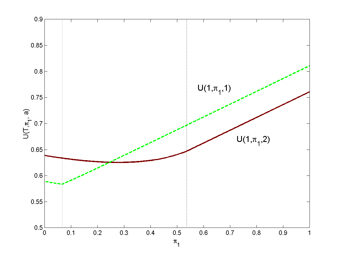
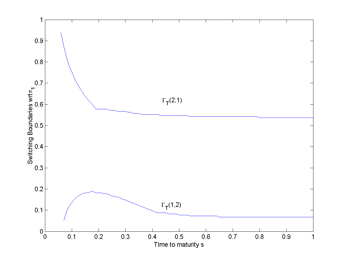
Figure 1. Sequential tracking of a two-state Markov chain. The left panel shows the value functions $U(T,\vec{\pi},\cdot)$, $a\in\{1,2\}$, as a function of $\pi_{1}$ for $T=1$. Recall that in this case $D=\{(\pi_{1},1-\pi_{1})\colon 0\leq\pi_{1}\leq 1\}$. The vertical lines indicate the boundary of $\Gamma_{T}(1,2)$ and $\Gamma_{T}(2,1)$. The right panel shows the switching regions $\Gamma_{s}(a,b)$ (namely $\Gamma_{s}(1,2)$ is below the lower curve and $\Gamma_{s}(2,1)$ is above the higher curve) as a function of time to maturity $s$.

6.2. Policy Making Example.

The Federal Reserve Board (the Fed) has the task of adjusting the US monetary policy in response to economic events. The Fed has authority over the overnight interest rates and attempts to implement a loose monetary policy when the economy is weak, and a tight monetary policy when the economy is overheating. Unfortunately, the current state of the economy $M$ is never precisely known; thus the main task of the Fed is to estimate $M$ from various economic information it collects. When the beliefs of the Fed change sufficiently, it will adjust its monetary policy $\xi$. Such adjustments are expensive, since they are closely followed by market participants and send out important signals to economic agents. Thus, beyond trying to track $M$, the Fed also seeks stability in its policies, in order not to disrupt planning activities of businesses.

As can be seen from this description, this problem fits well into our tracking paradigm of (1.3). For concreteness, let $M=\{M_{t}\}_{t\geq 0}$ represent the current economy with state space $E=\{1,2,3\}\equiv\{Overheating,Growth,Recession\}$. The generator of $M$ is taken to be

$$Q=\begin{pmatrix}-4&3&1\\ 2&-4&2\\ 0&3&-3\end{pmatrix}.$$

Thus, $M$ moves randomly between all three states (and we assumed that a recession cannot be immediately followed by overheating). In the face of these three states, the Fed also has three policy levels, namely its action set is $\mathcal{A}=\{0,1,2\}=\{Tight,Normal,Accommodating\}$.

The cost function $C(\vec{\pi},a)=\sum_{i\in E}c_{i}(a)\pi_{i}$, is given by the matrix

$$c_{i}(a)=c_{i,a}=\begin{bmatrix}2&-1&-1\\ 0&2&0\\ -1&-1&0\end{bmatrix},\qquad\qquad i\in E,a\in\mathcal{A}.$$

The switching costs are given by $K(a,b)=0.05\cdot 1_{\{a\neq b\}}$ for $a,b\in\mathcal{A}$. The observation process $X$ is a simple Poisson process with $M$-modulated intensity $\vec{\lambda}=[\lambda_{1},\lambda_{2},\lambda_{3}]=[1,2,5]$. Thus, the worse the economy state, the more frequent are (negative) events observed by the Fed.

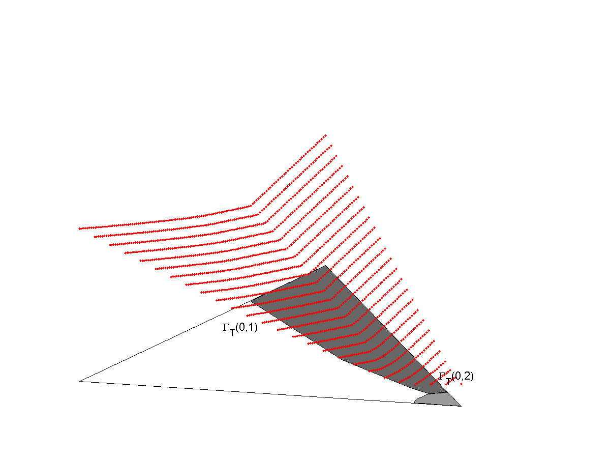
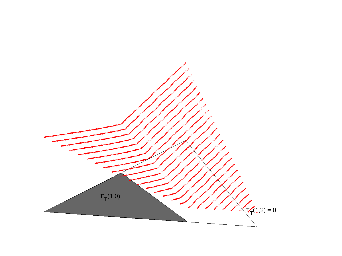
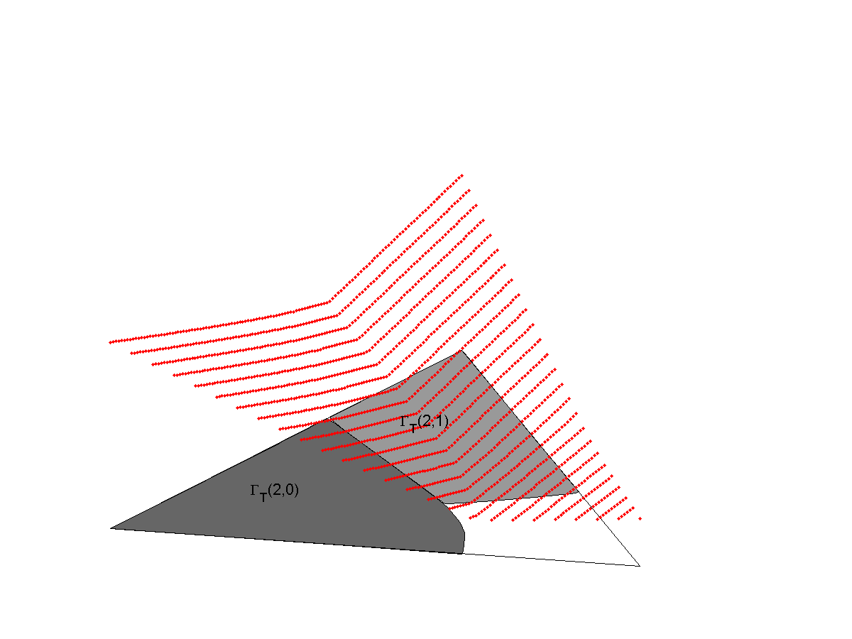
$a=0$ $a=1$ $a=2$

Figure 2. Value function $U(T,\vec{\pi},a)$ of the Fed policy-making example in Section 6.2 plotted together with the switching regions $\Gamma_{T}(a,\cdot)$ for each current policy $a$.

Figure 2 illustrates the obtained results for $T=4$ and no discounting. The triangular regions in Figure 2 are the state space $D=\{\vec{\pi}\in\mathbb{R}_{+}^{3}:\,\pi_{Ovr}+\pi_{Gro}+\pi_{Rec}=1\}$. The respective panels show how the initial switching regions $\Gamma_{T}(a,\cdot)$ and value functions $U(T,\vec{\pi},a)$ depend on the current policy $a$. Observe that because the penalty for not tracking recessions is small, starting out in the ‘Normal’ regime, the Fed will never immediately adopt an ‘Accommodating’ policy, $\Gamma_{T}(1,2)=\varnothing$. Similarly, because the penalty for missing an overheating economy is very large, the switching regions into a ‘Tight’ policy are large and conversely, the continuation region $\mathcal{C}_{T}(0)$ is large. Also, observe that the value function appears to be not differentiable at the boundaries. Finally, we stress that because of the final horizon, this problem is again non-time-stationary and the solution (as well as $\Gamma_{T}(a,\cdot)$) depends on remaining time $T$.

6.3. Customer Call Center Example

Our last example illustrates the structure of the infinite horizon version together with a different cost structure. We consider a call center application that employs a variable number of servers to answer calls. The calling rate fluctuates and is modulated by the unknown environment variable $M$. Having more servers decreases the per-call costs, but increases fixed costs related to payroll overhead.

We assume that $M_{t}\in E=\{Low,Med,High\}$ with a generator

$$Q=\begin{pmatrix}-1&1&0\\ 1&-2&1\\ 0&1&-1\end{pmatrix}.$$

The observed process $X$ represents the actual received calls and is taken to be a compound Poisson process with intensity $\lambda(M_{t})$ and marks $Y_{1},Y_{2},\ldots$ that represent intrinsic call costs. Suppose that $Y\in\{6,12,24\}$, and the distribution of $Y$ and $\lambda$ is $M$-modulated:

$$\nu_{i,j}=\mathbb{P}\{Y=y_{j}|M_{t}=i\}=\begin{pmatrix}1/4&1/2&1/4\\ 1/3&1/3&1/3\\ 1/4&1/4&1/2\end{pmatrix};\qquad\vec{\lambda}=[1\quad 3\quad 4].$$

Thus, as the manager receives calls, she dynamically updates her beliefs about current state of $M$ based on the intervals between call times and observed call types.

The call center manager can choose one of two strategies, namely she can employ either one or two agents, $a\in\mathcal{A}=\{1,2\}$. Employing $a$ agents leads to per-call costs of $c_{1}(Y,a)=-Y/a$ and to continuously-assessed costs of $c_{2}(Y,a)=-(10+20a)$. Thus, when $\mathbb{P}\{M_{t}=High\}$ is sufficiently high, it is optimal to employ both agents, otherwise one is sufficient. Finally, switching costs for increasing or decreasing number of agents are set at $K(a,b)=2$. Note that here all the costs are independent of $M$ (and hence of $\vec{\Pi}$).

We consider an infinite horizon formulation and take $\rho=0.5$. The parameter $\rho$ measures the trade-off between minimizing immediate costs and having a long-term strategy that takes into account future changes in $M$. Thus $\rho=0.5$ means that the horizon of the controller is on the time-scale of two time periods. The overall objective is:

$$\sup_{\xi\in\mathcal{U}(\infty)}\mathbb{E}^{\vec{\pi},a}\left[\sum_{j=1}^{\infty}\mathrm{e}^{-\rho\sigma_{j}}c_{1}(Y_{j},\xi_{\sigma_{j}})+\int_{0}^{\infty}\mathrm{e}^{-\rho t}c_{2}(\xi_{t})\,dt-\sum_{k}\mathrm{e}^{-\rho\tau_{k}}K(\xi_{k-1},\xi_{k})\right].$$

Figure 3 shows the results, as well as a computed color-coded sample path of $\vec{\Pi}$ which shows the implemented optimal strategy. The given path has four jumps and three policy changes (two changes occur between jumps when $\vec{\Pi}$ enters $\Gamma(1,2)$, and one change occurs at an arrival when $\vec{\Pi}$ jumps back into $\Gamma(2,1)$). Observe that in the absence of new information, $\vec{\Pi}$ converges to the fixed point $\vec{\pi}_{\infty}=[0.7,0.23,0.07]$ (the invariant distribution of $\mathrm{e}^{Q-\Lambda}$), as can be seen from the flow of the paths in Figure 3.

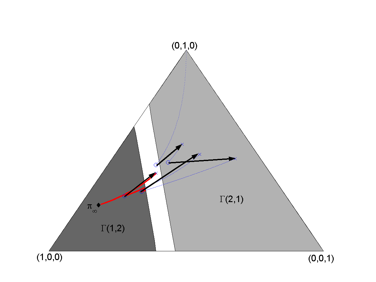
Figure 3. Tracking the regime of a customer call center. We show a sample path of $\vec{\Pi}$ inside the simplex $D=\{(\pi_{1},\pi_{2},\pi_{3}):\pi_{i}\geq 0,\pi_{1}+\pi_{2}+\pi_{3}=1\}$, as well as the corresponding optimal strategy. The initial state is $\vec{\Pi}_{0}=(0,1,0)$ and $\xi_{0}=1$. On this path we have $t\in[0,4]$ and the arrival pairs (corresponding to jumps of $X$, recall $\vec{\Pi}$-dynamics in (2.13)) $(\sigma_{\ell},Y_{\ell})$ for $\ell=1,2,3,4$ are $(0.51,2),(0.66,3),(1.44,1),(2.23,2)$, respectively. The resulting optimal strategy $\xi^{*}$ is color-coded: dashed line for $\xi^{*}_{t}=1$, solid line for $\xi^{*}_{t}=2$.

References

- Aggoun (2003) L. Aggoun. Optimal tracking for an insurance model. Stochastic Anal. Appl., 21(6):1207–1214, 2003. ISSN 0736-2994.
- Arjas et al. (1992) E. Arjas, P. Haara, and I. Norros. Filtering the histories of a partially observed marked point process. Stochastic Process. Appl., 40(2):225–250, 1992. ISSN 0304-4149.
- Bayraktar and Dayanik (2006) E. Bayraktar and S. Dayanik. Poisson disorder problem with exponential penalty for delay. Mathematics of Operations Research, 31 (2):217–233, 2006.
- Bayraktar and Sezer (2006) E. Bayraktar and S. Sezer. Quickest detection for a Poisson process with a phase-type change-time distribution. Technical report, University of Michigan, 2006. URL http://arxiv.org/abs/math/0611563.
- Bayraktar et al. (2006) E. Bayraktar, S. Dayanik, and I. Karatzas. Adaptive Poisson disorder problem. Annals of Applied Probability, 16 (3):1190–1261, 2006.
- Bremaud (1981) P. Bremaud. Point Processes and Queues. Springer, New York, 1981.
- Ceci and Gerardi (1998) C. Ceci and A. Gerardi. Partially observed control of a Markov jump process with counting observations: equivalence with the separated problem. Stochastic Processes and Applications, 78:245–260, 1998.
- Chopin and Varini (2007) N. Chopin and E. Varini. Particle filtering for continuous-time hidden Markov models. ESAIM Proceedings, 19:12–17, 2007. Conférence Oxford sur les méthodes de Monte Carlo séquentielles.
- Costa and Davis (1988) O. L. V. Costa and M. H. A. Davis. Approximations for optimal stopping of a piecewise-deterministic process. Math. Control Signals Systems, 1(2):123–146, 1988. ISSN 0932-4194.
- Costa and Davis (1989) O. L. V. Costa and M. H. A. Davis. Impulse control of piecewise-deterministic processes. Math. Control Signals Systems, 2(3):187–206, 1989. ISSN 0932-4194.
- Costa and Raymundo (2000) O. L. V. Costa and C. A. B. Raymundo. Impulse and continuous control of piecewise deterministic Markov processes. Stochastics Stochastics Rep., 70(1-2):75–107, 2000. ISSN 1045-1129.
- Darroch and Morris (1968) J. N. Darroch and K. W. Morris. Passage-time generating functions for continuous-time finite Markov chains. Journal of Applied Probability, 5(2):414–426, 1968.
- Davis (1993) M. H. A. Davis. Markov Models and Optimization. Chapman & Hall, London, 1993.
- Elliott et al. (1995) R. J. Elliott, L. Aggoun, and J. B. Moore. Hidden Markov models, volume 29 of Applications of Mathematics. Springer-Verlag, New York, 1995. ISBN 0-387-94364-1. Estimation and control.
- Gugerli (1986) U. Gugerli. Optimal stopping of a piecewise-deterministic Markov process. Stochastics, 19(4):221–236, 1986.
- Jacod and Shiryaev (1987) J. Jacod and A. Shiryaev. Limit Theorems for Stochastic Processes. Springer-Verlag, Berlin, 1987.
- Karlin and Taylor (1981) S. Karlin and H. M. Taylor. A second course in stochastic processes. Academic Press, New York, 1981. ISBN 0-12-398650-8.
- Lenhart and Liao (1988) S. M. Lenhart and Y. C. Liao. Switching control of piecewise-deterministic processes. J. Optim. Theory Appl., 59(1):99–115, 1988.
- Ludkovski and Sezer (2007) M. Ludkovski and S. Sezer. Finite horizon decision timing with partially observable Poisson processes. Technical report, University of Michigan, 2007.
- Mazziotto et al. (1988) G. Mazziotto, Ł. Stettner, J. Szpirglas, and J. Zabczyk. On impulse control with partial observation. SIAM J. Control Optim., 26(4):964–984, 1988. ISSN 0363-0129.
- Muller et al. (2004) P. Muller, B. Sanso, and M. De Iorio. Optimal Bayesian design by inhomogeneous Markov chain simulation. Journal of the American Statistical Association, 99:788–798, 2004.
- Neuts (1989) M. F. Neuts. Structured Stochastic Matrices of M/G/1 Type and Their Applications. Marcel Dekker, New York, 1989.
- Peskir and Shiryaev (2002) G. Peskir and A. N. Shiryaev. Solving the Poisson disorder problem. In Advances in Finance and Stochastics, pages 295–312. Springer, New York, 2002.
- Peskir and Shiryaev (2000) G. Peskir and A. N. Shiryaev. Sequential testing problems for Poisson processes. Annals of Statistics, 28:837–859, 2000.
- Shiryaev (1978) A. N. Shiryaev. Optimal stopping rules. Springer-Verlag, Berlin, 1978.
- Tartakovsky et al. (2006) A. G. Tartakovsky, B. L. Rozovskii, R. B. Blažek, and H. Kim. Detection of intrusions in information systems by sequential change-point methods. Stat. Methodol., 3(3):252–293, 2006. ISSN 1572-3127.