How does the scaling for the polymer chain in the dissipative particle dynamics hold?
Abstract
We performed a series of simulations for a linear polymer chain in a solvent using dissipative particle dynamics to check the scaling relations for the end-to-end distance, radius of gyration and hydrodynamic radius in three dimensions. The polymer chains of up to beads in explicit solvent of various quality are studied. To extract the scaling exponent , the data are analyzed using linear fits, correction-to-scaling forms and analytical fits to the histograms of radius of gyration distribution. For certain combinations of the polymer characteristics and solvent quality, the correction-to-scaling terms are found to be essential while for the others these are negligibly small. In each particular case the final value for the exponent was chosen according to the best least-squares fit. The values of obtained in this way are found within the interval but are concentrated mostly around , which is very close to the best known theoretical result . The existence of this interval is attributed both to the peculiarities of the method and to the moderate chain lengths being simulated. Within this shortcoming, the polymer chain in this kind of modeling is found to satisfy the scaling relations for all three radii being considered
Key words: polymers, scaling, scaling exponents, dissipative particle dynamics
PACS: 61.25.Hq, 61.20.Ja, 89.75.Da
1 Introduction
Variety of physical, chemical, and biological phenomena which involve polymers as well as variety of polymer characteristics one is interested in have been naturally reflected in numerous theoretical methods and models used for polymer description [1]. In particular, it is generally recognized by now, that the scaling properties of a long flexible polymer chain immersed in a good solvent are perfectly described by the model of self-avoiding walks (SAW) [2]. A textbook example is given by the mean square end-to-end distance of a SAW of steps and that of a linear polymer chain, either of which scales in an asymptotic limit as:
| (1) |
with a universal exponent . The value of the exponent depends on the space dimension only and is the same for all SAW on different three dimensional (3d) lattices. Relation (1) is violated for the finite and an approach to the asymptotics is governed by the corrections to scaling. With an account of the first correction equation (1) reads:
| (2) |
Here , are non-universal amplitudes and is an universal correction-to-scaling exponent. Theoretical estimates for the exponents follow from the field theoretical renormalization group calculations [3]:
| (3) |
Whereas the SAW on the discrete lattice is a perfect model to study scaling of long flexible polymer chains in a good solvent [4], for obvious reasons it fails to describe most of the other properties of the chain [1, 5]. A more realistic model would be defined in a continuous space and involves both monomer-monomer and monomer-solvent interactions. Brownian dynamics is one of the candidates, as it operates on the mesoscale and incorporates the random force acting on each monomer which mimics the effect of a solvent [6]. However, the method lacks correct hydrodynamics limit. Similar but more rigorous technique, i.e., the dissipative particles dynamics (DPD), was introduced by Hoogerbrugge and Koelman [7] and later refined by Español and Warren to satisfy the detailed balance [8]. The method has correct hydrodynamics limit [9] and quickly gained much attention as a powerful technique for mesoscale simulations of various kinds of macromolecules [6].
Therefore, an important issue of analysis is to check how the scaling laws (e.g. of equation (1) form) hold in the case of the DPD-based simulations. This issue was partly considered in [10, 11, 12, 13, 14]. However, some issues remain unclear (see the next section 2 for details). We see a good reason to discuss in detail the scaling laws for the polymer chain in a solvent in the DPD method. As far as the method was successfully used for the simulations of branched, amphiphilic and other complex molecules, the validation of correct scaling laws on such a well-studied system as linear chain polymer would be a strong supporting factor for extending the subject to the scaling laws in more complex systems (e.g. star-like, branched, dendritic systems, etc.).
2 Previous simulations
A number of various simulation techniques have been used to numerically verify the scaling laws of the polymer in solution, namely the molecular dynamics (MD), Monte Carlo (MC), DPD and others. Here we shall provide a rather brief account of references relevant to the present study.
By using the MC method enriched by special techniques, one can move very efficiently through the conformational space (see, e.g. [6]). As the result, the method is quite suitable for the simulations of random walks (RW) and SAW [15, 16]. Li et al. [16] used a pivot algorithm and other techniques applied to the chain of monomers. The value for the scaling exponent obtained is and it agrees very well with the theoretical estimate (3). To study dynamical properties, however, one should turn to true dynamical methods. Pierleone and Ryckaert [17] performed a comprehensive analysis of the scaling laws for both static (radius of gyration, and end-to-end distance ) and dynamical (diffusion coefficient, ) properties using MD simulations. One of the important outcomes is that the static properties are unaffected by the finiteness of the box size providing that . The scaling exponent values and (for the and , respectively) were obtained. On the contrary, dynamical properties were found to be strongly dependent on . This fact was explained by hydrodynamic interactions of the chain with its own images due to the periodic boundary conditions (PBC). If, following Dunweg and Kremer[18] one uses the Kirkwood formula, then a correct dynamical scaling is also recovered [17].
A number of simulations of linear polymers using DPD technique are available. Schlijper et al. [10] were the first to study static and dynamic scaling laws for the DPD chain in athermal solvent. Later their results for this case were confirmed and extended to include the solvents of variable quality by Kong et al. [11]. These authors studied (among the other properties) and have found for the athermal solvent which is closer to the polymer at the -condition. With the increase of solvent quality, the value close to a SAW exponent was recovered. This problem was further addressed by Spenley [12] who studied the in polymer melt and solution. In the latter case, relevant to our study, the exponent was obtained. The previous result by Kong et al.[11] was commented as being influenced by the type of spring potential used there. In our opinion, this discrepancy could also be due to insufficient statistics.
It has also been debated whether the soft repulsion inherent to the DPD method is sufficient to model the self-avoidance of the chains. In particular, Symeonidis et al. [13] used additional intramolecular interactions (e.g. Lennard-Jones-like repulsion term) to increase the chain self-avoidance and experimented with different forms of the bond springs (i.e. FENE, Hookean and WLC). One of the conclusions made by the authors is, that the presence of FENE potential alone ensures a correct value for the exponent and no extra interactions for the improvement of self-avoidance are required.
Jiang et al. [14] have carried out an extensive study of the hydrodynamical properties obtained via the DPD method. In particular, scaling laws for both and for the dilute athermal solution are relevant to our study. The authors found the values for the scaling exponent weakly dependent on the box size with the averages of for the radius of gyration and for the end-to-end distance[14] (the box sizes of DPD length units were used and a range of chain lengths was DPD beads). The other conclusion given in [14] is the one already mentioned above, claiming that the original soft interactions are sufficient for self-avoidance of the chains in the DPD method. Similarly to the MD study of Pierleone and Ryckaert [17], the diffusion coefficient was found to be highly sensitive to the simulational box size. However, after the appropriate corrections to the system size were introduced, the scaling law for the diffusion coefficient was obtained. Since, according to Kirkwood theory, the diffusion coefficient is related to the hydrodynamic radius [18], the latter is also shown to obey the correct scaling law.
Despite the availability of simulational studies that concentrate on static and dynamical scaling of the polymer in DPD method, there are still certain points that need to be clarified, namely:
-
(i)
do all the relevant radii, , and scale with the same scaling exponent ?
-
(ii)
are the corrections to scaling relevant and can these improve the results or make these more consistent?
-
(iii)
in case of a good solvent, will the changes in the polymer-solvent interaction potential lead to any detectable drift of the scaling exponent ?
These three points will be addressed in the current study.
3 Simulational details
In our study we closely follow the DPD method as discussed by Groot and Warren [19]. Polymer molecule (see, figure 1) is modeled as a chain of soft beads connected via harmonic springs. The bonding force acting on the -th bead from its bond neighbour is:
| (4) |
where , , and is the spring constant. Here and thereafter, the length, mass, time and energy () units are chosen to be equal to unity.

The solvent is described in an explicit way, in a form of isolated beads of the same origin as the polymer ones (see, figure 1). Each -th bead (polymer or solvent one) is subject to a pairwise non-bonded force from its -th counterpart. The force acting on the -th bead due to the interaction with the -th bead consists of three contributions:
| (5) |
where the conservative , dissipative and random contributions are of the following form:
| (6) |
| (7) |
Here , and being the velocities of the beads, is Gaussian random variable: , . According to Español and Warren [8], the dissipative and random force amplitudes are interrelated, and , to satisfy the detailed balance. The frequently used analytical form is:
| (8) |
We choose the value . Parameter in the conservative force defines maximum repulsion between two beads which occurs at complete overlap . Three different parameters can be distinguished, for the polymer-polymer, for the solvent-solvent and for the polymer-solvent interactions and all these can be varied. As was shown in [19], these parameters can be related to the Flory-Huggins parameter . To integrate the equations of motion, we used the modified velocity–Verlet algorithm by Groot and Warren [19]. Let us note that the structural properties of the chain in a solvent are defined solely by the conservative forces (6), while the dissipative and random forces (7) govern the phase space trajectory.
In our DPD simulations we considered the following set of chain lengths: , , , , , , , and beads in four types of solvent:
| (9) |
The terms ‘‘good’’ and ‘‘very good’’ are indicative rather than exact, since only repulsive forces are taken into account in DPD. Hence, ‘‘good solvent’’ means less repulsion for the polymer-solvent interaction than that for the polymer-polymer one. The last two cases in equations (9) correspond to the values and , respectively, in notation of Kong et al. [11].
All the simulations were performed in ensemble. At first, the initial chain conformation was generated as a RW. Then, it was immersed into a relatively large box filled by solvent and short preliminary runs were performed to estimate the approximate for the polymer. Thereafter, the final run was performed using the cubic box of the linear size . This size is considered to be sufficiently large to eliminate the effects of PBC [14, 17]. The number of solvent beads was chosen to keep the total reduced density of the solution equal to . The time step was chosen to be in reduced units. We performed from (for ) up to (for ) DPD steps for the final run. We did not concentrate on the relaxation times in detail, but found the behaviour similar to Jiang et al. [14], who used similar DPD parameters for athermal solvent. This brings us to the following estimates for the simulation runs: about for and for with the estimates for intermediate values of falling in between. The chain conformations were saved after performing every DPD steps and last of these were used for the subsequent analysis. As far as all the simulations were performed using PBC, the unwrapping of the chain at each time step was performed based on the connectivity information.
4 Results
We concentrated our analysis on the three following metric characteristics of the linear polymer. The instantaneous squared end-to-end distance at a given time is defined as:
| (10) |
where and are the radius-vectors for the first and last bead of the chain, respectively. The squared radius of gyration at time is defined as:
| (11) |
where is the radius-vector of the polymer center of mass. The inverse hydrodynamic radius is defined as follows:
| (12) |
where the sum runs over all different bead pairs . All three properties are time averaged (denoted hereafter as ) and then the first two can be square rooted while the third one is inverted to provide the estimates for , and , respectively.
One should consider and as more useful characteristics as compared to . First of all, is meaningful for the linear polymer or for a certain subchain of the branched molecule (e.g. backbone, side chain, star-polymer arm, etc.), while both and are universally defined. Apart from that, both these properties are directly measurable via small-angle scattering experiments and via small-angle dynamic light scattering experiments, respectively (for more discussion on this, see [20]).
4.1 Linear fit and first correction-to-scaling fit
As was already mentioned above, a number of universal scaling laws have been observed for the polymer properties [2] in the limit of infinite polymer length, e.g. equations (1). To reproduce these properties, one needs to consider rather long chains in the simulations [16]. Due to the polymer coil self-similarity, one would expect that such a coarse-grained approach as DPD should be capable of reproducing correct scaling laws for much shorter chain lengths. For the moderate polymer lengths, usually the scaling is written in terms of a number of bonds, , instead of the number of monomers . Also, as is known, the correction-to-scaling terms are important for moderate system sizes, as is indicated by the studies of the phase transitions in spin lattice models [21, 22, 23]. Taking into account the first correction-to-scaling term, equation (2), one has for the :
| (13) |
We shall work with square rooted values
| (14) |
and keep the linear term only in the correction-to-scaling expansion above. Taking a logarithm of both sides of equations (14), we obtain
| (15) | |||||
where and are self-explanatory. The same formulae can also be applied for and (in the latter case one has ). As a result, the same fit (15) can be used for all three quantities under interest, , and . In the case of linear fit the correction-to-scaling amplitude is assumed to be zero and one recovers the linear fit form. To perform the fits we used the least-squares routine mrqmin from the Numerical recipes book [24]. The accuracy of the fit was monitored by the cumulative squared deviation per one data point,
| (16) |
where (,) is the -th out of data points and is the fitting function.
It is generally known that very good statistics for each data point are required to ensure robust results for the scaling exponent . Otherwise the latter depends essentially on the selection of data points being used for the fit. This was also found to be the case in the course of the present study. Hence, relatively lengthly simulations are performed to improve statistics. To check the consistency of the results, we performed a series of fits using a gradually increasing range of intervals in the chain length , e.g. , which are presented below.
As was anticipated, both cases of ‘‘athermal 1’’ and ‘‘athermal 2’’ solvents were found to show the same averaged properties within the accuracy of the simulations. Therefore, the data for both cases have been averaged at each and marked as ‘‘athermal’’ further in the text. At first glance, the data points for both and are well fitted by the line in log-log scale (see, figure 2), but, in fact, the best fits were achieved using the first correction-to-scaling form (15). We should remark here that we were unable to achieve stable results for both and using the four-parameter fits, in which all , , and in (15) are fitted simultaneously. Instead, we were forced to fix the correction-to-scaling exponent at certain value and to perform the fit over three remaining parameters. We used two choices for , namely the best theoretical value [3] and .
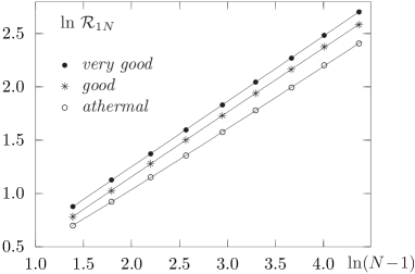
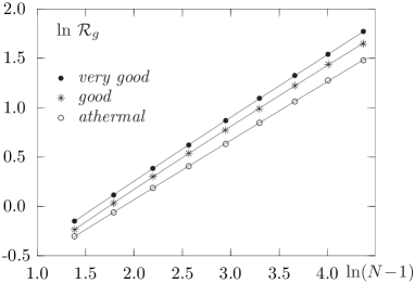
The results presented in table 1 indicate that the correction-to-scaling term for is essential in the case of athermal solvent only. In the table, we also show the linear fit performed over the largest chain lengths, , for the sake of comparison. One can see that the latter leads to almost the same result as the correction-to-scaling fit , which is indicative of the crossover quickly decreasing at . In the cases of good and very good solvents very small amplitudes are found and, as the result, linear fits are almost equally good (see, table 1). For the situation is exactly reversed. The correction to scaling is important for the cases of good and very good solvents (see, table 2). We cannot suggest some definite explanation for this effect, except the conclusion that preference should be given to the general form (15), rather than to the linear fit, otherwise the exponent could be essentially under- or overestimated (see, tables 1, 2).
| fitting | linear fit | fit with | fit with |
| range, | |||
| athermal solvent | |||
| 5 28 | 0.564 1.7e–5 | 0.617 [0.370] 9.4e–7 | 0.588 [0.219] 1.3e–6 |
| 5 40 | 0.569 3.1e–5 | 0.621 [0.399] 9.0e–7 | 0.592 [0.252] 1.8e–6 |
| 5 56 | 0.573 5.5e–5 | 0.627 [0.447] 1.3e–6 | 0.596 [0.295] 3.6e–6 |
| 5 80 | 0.574 5.2e–5 | 0.611 [0.318] 8.2e–6 | 0.591 [0.248] 6.9e–6 |
| 20 80 | 0.586 8.6e–6 | ||
| good solvent | |||
| 5 28 | 0.607 8.6e–6 | 0.591 [–0.099] 6.4e–6 | 0.600 [–0.066] 6.9e–6 |
| 5 40 | 0.607 7.7e–6 | 0.595 [–0.076] 5.7e–6 | 0.601 [–0.056] 6.0e–6 |
| 5 56 | 0.607 7.3e–6 | 0.604 [–0.026] 7.0e–6 | 0.605 [–0.023] 7.0e–6 |
| 5 80 | 0.605 1.7e–5 | 0.594 [–0.087] 1.1e–5 | 0.600 [–0.073] 1.2e–5 |
| 20 80 | 0.601 1.5e–5 | ||
| very good solvent | |||
| 5 28 | 0.614 6.3e–7 | 0.610 [–0.021] 5.4e–7 | 0.612 [–0.019] 5.0e–7 |
| 5 40 | 0.613 1.7e–6 | 0.605 [–0.052] 8.3e–7 | 0.609 [–0.041] 8.4e–7 |
| 5 56 | 0.613 2.1e–6 | 0.612 [–0.009] 2.1e–6 | 0.612 [–0.011] 2.1e–6 |
| 5 80 | 0.613 2.0e–6 | 0.611 [–0.012] 1.9e–6 | 0.612 [–0.012] 1.8e–6 |
| 20 80 | 0.613 2.8e–6 | ||
| fitting | linear fit | fit with | fit with |
| range, | |||
| athermal solvent | |||
| 5 28 | 0.601 2.7e–6 | 0.584 [–0.106] 2.0e–7 | 0.592 [–0.080] 2.5e–7 |
| 5 40 | 0.600 3.1e–6 | 0.587 [–0.090] 3.0e–7 | 0.593 [–0.073] 2.6e–7 |
| 5 56 | 0.600 2.8e–6 | 0.593 [–0.052] 1.5e–6 | 0.597 [–0.047] 1.3e–6 |
| 5 80 | 0.599 8.0e–6 | 0.587 [–0.087] 2.9e–6 | 0.593 [–0.077] 3.1e–6 |
| 20 80 | 0.596 6.0e–6 | ||
| good solvent | |||
| 5 28 | 0.641 4.9e–5 | 0.573 [–0.368] 2.7e–6 | 0.605 [–0.318] 4.2e–6 |
| 5 40 | 0.638 5.3e–5 | 0.586 [–0.314] 5.4e–6 | 0.610 [–0.283] 5.0e–6 |
| 5 56 | 0.636 5.1e–5 | 0.597 [–0.260] 9.4e–6 | 0.615 [–0.244] 7.3e–6 |
| 5 80 | 0.631 9.7e–5 | 0.588 [–0.306] 1.4e–5 | 0.609 [–0.299] 1.4e–5 |
| 20 80 | 0.618 2.8e–5 | ||
| very good solvent | |||
| 5 28 | 0.651 6.9e–6 | 0.626 [–0.144] 1.9e–6 | 0.639 [–0.109] 2.2e–6 |
| 5 40 | 0.647 1.6e–5 | 0.618 [–0.185] 2.6e–6 | 0.633 [–0.151] 3.6e–6 |
| 5 56 | 0.645 2.4e–5 | 0.616 [–0.194] 2.4e–6 | 0.631 [–0.168] 3.7e–6 |
| 5 80 | 0.642 3.4e–5 | 0.615 [–0.201] 2.2e–6 | 0.629 [–0.184] 3.9e–6 |
| 20 80 | 0.632 2.3e–6 | ||
| fitting | fit with | four-parameter fit |
| range, | ||
| athermal solvent | ||
| 5 28 | 0.596 [3.008] 4.9e–5 | 0.497 0.836 [1.324] 1.9e–7 |
| 5 40 | 0.611 [3.275] 6.9e–5 | 0.534 0.732 [1.683] 4.7e–7 |
| 5 56 | 0.625 [3.555] 9.5e–5 | 0.572 0.666 [2.195] 1.0e–6 |
| 5 80 | 0.635 [3.786] 1.0e–4 | 0.552 0.699 [1.912] 1.2e–6 |
| good solvent | ||
| 5 28 | 0.623 [2.953] 2.0e–5 | 0.476 1.017 [0.925] 4.8e–7 |
| 5 40 | 0.639 [3.274] 3.1e–5 | 0.563 0.654 [1.636] 2.3e–6 |
| 5 56 | 0.654 [3.592] 5.1e–5 | 0.641 0.577 [2.993] 3.0e–6 |
| 5 80 | 0.658 [3.710] 4.7e–5 | 0.565 0.664 [1.663] 5.5e–6 |
| very good solvent | ||
| 5 28 | 0.625 [3.052] 5.9e–5 | 0.652 0.643 [3.159] 1.5e–7 |
| 5 40 | 0.639 [3.284] 7.8e–5 | 0.580 0.703 [1.925] 6.1e–7 |
| 5 56 | 0.651 [3.533] 9.7e–5 | 0.583 0.698 [1.963] 5.4e–7 |
| 5 80 | 0.662 [3.779] 1.1e–4 | 0.577 0.710 [1.885] 5.1e–7 |
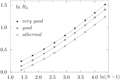
The four-parameter fit, mentioned above, does not work for either or but is supposed to perform better for , where essentially larger correction to scaling is to be expected [20]. Indeed, this is found to be the case in our simulations. First of all, this can be noticed from the arrangement of the data points, see figure 3. The results based on numerical fits are presented in table 3, where both the cases of fixed and of the four-parameter fits are shown. The latter give essentially better results in terms of fitting accuracy and provide independent estimates for both exponents, and . As was demonstrated by Dunweg et al. [20] there are two comparable correction-to-scaling terms for the , one is proportional to and another, the so-called ‘‘analytic’’ correction, is proportional to . Therefore, if one uses the form (15) with a single correction term, then a rather effective exponent will be obtained. This is how we should interpret the value obtained in our study.
4.2 The fits based on the distribution of values
The averaging of the metric properties of interest, e.g. , throughout this study was performed as the arithmetic mean over discrete set of time points. One can also be interested in the distribution of the values themselves and, for instance, in examination of the scaling law for the most probable values with the chain length . The following analytical form has been postulated by Lhuillier in 3d [25]
| (17) |
where , and , are constants. Subsequently, this has been verified in a number of lattice MC simulations [26, 27]. One can rewrite this distribution in terms of , using the expressions for and and incorporating the -dependent factors into the constants, and the result reads:
| (18) |
This distribution has a maximum at
| (19) |
which can be square rooted to obtain an estimate for the most probable value of the radius of gyration . We prefer to work with the distribution of (18) and then to square root the maximum to match the averaging procedure for simple averaging, .
From the point of view of numerical fitting, the form (18) has four parameters: one exponent and three coefficients, , and . Therefore, one can have a first estimate for the exponent right from the fit of the data to the form (18). The second estimate for can be obtained from the anticipated scaling of according to the form (15).
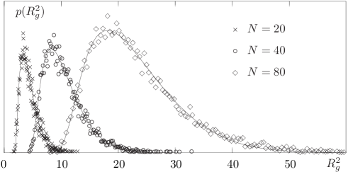
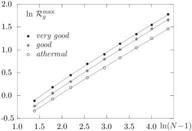
The distributions were built in a form of histograms and were found to map very well on the Lhuillier form (18), see samples in figure 4 obtained for the case of athermal solvent. These fits, as was mentioned above, provide both the estimate for and an independent estimate for the exponent . The latter was found to be scattered in the interval depending on and solvent type. We do not expect high accuracy from such a fitting, as far as dependence on in equations (18) is rather complex. Nevertheless, the values of found are very reasonable and indicate a self-consistency of this numerical approach. The next step is to use the maxima positions of the distributions (18), found via equations (19), and to find a fit to the scaling law (15) similarly to the analysis of data in the previous subsection. The data points alongside with the best fits are shown in figure 5 and the results for the exponent , correction-to-scaling amplitude and fitting error are presented in table 4. We would like to stress that, contrary to the results given in table 2, no dependence on solvent quality is observed in table 4 and the same value is found essentially in all three cases. This might indicate that the effect of small drift of observed in a very good solvent in table 2 could be an artefact of the numerical method used.
| fitting | linear fit | fit with | fit with |
| range, | |||
| athermal solvent | |||
| 5 28 | 0.602 6.4e–5 | 0.539 [–0.345] 2.6e–5 | 0.568 [–0.306] 2.4e–5 |
| 5 40 | 0.601 5.6e–5 | 0.562 [–0.242] 3.2e–5 | 0.579 [–0.222] 2.8e–5 |
| 5 56 | 0.601 4.9e–5 | 0.576 [–0.169] 3.4e–5 | 0.587 [–0.165] 3.0e–5 |
| 5 80 | 0.598 5.6e–5 | 0.574 [–0.183] 3.1e–5 | 0.585 [–0.181] 2.7e–5 |
| 20 80 | 0.598 2.3e–5 | ||
| good solvent | |||
| 5 28 | 0.646 4.6e–5 | 0.594 [–0.291] 2.1e–5 | 0.618 [–0.247] 2.0e–5 |
| 5 40 | 0.641 6.6e–5 | 0.588 [–0.316] 1.8e–5 | 0.613 [–0.283] 1.9e–5 |
| 5 56 | 0.640 5.9e–5 | 0.606 [–0.231] 2.7e–5 | 0.622 [–0.217] 2.5e–5 |
| 5 80 | 0.633 1.8e–4 | 0.582 [–0.352] 6.2e–5 | 0.607 [–0.344] 6.9e–5 |
| 20 80 | 0.609 9.4e–5 | ||
| very good solvent | |||
| 5 28 | 0.646 2.6e–4 | 0.517 [–0.626] 6.0e–5 | 0.571 [–0.634] 5.5e–5 |
| 5 40 | 0.636 3.4e–4 | 0.522 [–0.610] 5.2e–5 | 0.570 [–0.637] 4.7e–5 |
| 5 56 | 0.628 3.8e–4 | 0.529 [–0.582] 4.9e–5 | 0.572 [–0.624] 4.2e–5 |
| 5 80 | 0.625 3.7e–4 | 0.549 [–0.503] 7.8e–5 | 0.582 [–0.551] 5.9e–5 |
| 20 80 | 0.607 3.9e–5 | ||
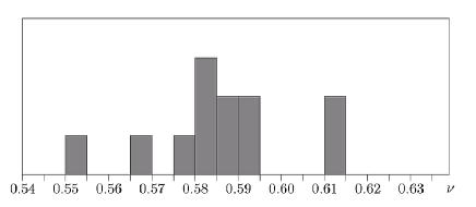
The cumulative outcome of our analysis for the scaling exponent which governs the scaling law (2) is presented in figure 6. Here we show a histogram of the values of obtained for , and of a polymer chain in different solvents considered in the current study, namely, in athermal, good and very good solvents. To make this histogram, the best fits (underlined results in tables 1–4) have been used. One can see from the histogram that the value of is scattered in an interval but in fact is found predominantly in much narrower interval centered around the best theoretical estimate [3]. This allows us to conclude that within the accuracy of our analysis, the scaling law (2) holds for all polymer characteristics and in all solvents considered in this study. Our conservative estimate for the scaling exponent therefore is
| (20) |
5 Conclusions and outlook
In this study we performed DPD simulations of the polymer chain in a solvent of various quality with the aim to reexamine how well the scaling laws hold for various polymer characteristics. Chains of up to beads were considered and simulation runs from up to relaxation times were performed. Three metric properties were considered, end-to-end distance, radius of gyration and hydrodynamic radius. For the analysis we used the linear fits, first correction-to-scaling fits and fitting the distribution of the radius of gyration. As an outcome, within the accuracy of the simulations and of the data analysis technique, the following conclusions can be drawn:
- (i)
-
(ii)
Corrections to scaling are found to be important in all combinations except a few property/solvent ones and thus the conclusion (i) is valid only when the correction-to-scaling terms are taken into account.
-
(iii)
No or very small (up to 4%) drift of the scaling exponent is observed when changing the solvent quality (remaining, however, in a good solvent regime), but this effect depends on a numerical technique being used.
The method of analysis can be extended to the study of the scaling laws in more complex molecular architectures, e.g. star-like polymers, branched and hyperbranched molecules (including amphiphiles).
Acknowledgements
We thank Prof. Myroslav Holovko for the invitation to contribute to the Festschrift dedicated to Prof. Fumio Hirata 60th birthday. Work of Yu.H. was supported in part by the Austrian Fonds zur Förderung der wissenschaftlichen Forschung under Project P 19583 and work of J.I. by DFG grant NE410/8-2.
References
- 1. des Cloizeaux J., Jannink G. Polymers in Solution. Clarendon Press, Oxford, 1990.
- 2. de Gennes P.-G. Scaling Concepts in Polymer Physics. Cornell University Press, Ithaca and London, 1979.
- 3. Guida R., Zinn-Justin J., J. Phys. A, 1998, 31, 8103.
- 4. Sokal A.D. Monte Carlo and Molecular Dynamics Simulations in Polymer Science, ed. by Binder K., Oxford University Press, New York, 1995.
- 5. Schäfer L. Universal Properties of Polymer Solutions as Explained by the Renormalization Group. Springer, Berlin, 1999.
- 6. Frenkel D., Smit B. Understanding molecular simulation: from algorithms to applications. Academic Press Inc., San Diego, 1996.
- 7. Hoogerbrugge P.J., Koelman J.M.V.A., Europhys. Lett., 1992, 19, 155.
- 8. Español P., Warren P., Europhys. Lett., 1995, 30, 191.
- 9. Ripoli M., Ernst M.H., Español D., J. Chem. Phys., 2001, 115, 7271.
- 10. Schlijper A.G., Hoogerbrugge P.J., Manke C.W., J. Rheology, 1995, 39, 567.
- 11. Kong Y., Manke C.W., Madden W.G., Schlijper A.G., J. Chem. Phys., 1997, 107, 592.
- 12. Spenley N.A., Europhys. Lett., 2000, 49, 534.
- 13. Symeonidis V., Karniadakis G.E., Caswell B., Phys. Rev. Lett., 2005, 95, 076001.
- 14. Jiang W., Huang J., Wang Y., Laradji M., J. Chem. Phys., 2007, 126, 044901.
- 15. Grassberger P., J. Phys., 1993, A26, 2769.
- 16. Li B., Madras N., Sokal A.D., J. Stat. Phys., 1995, 80, 661.
- 17. Pierleoni C., Ryckaert J.-P., J. Chem. Phys., 1992, 96, 8539.
- 18. Dunweg B., Kremer K., Phys. Rev. Lett., 1991, 61, 2996.
- 19. Groot R.D., Warren P.B., 1997, 107, 4423.
- 20. Dunweg B., Reith D., Steinhauser M., Kremer K., J. Chem. Phys., 2002, 117, 914.
- 21. Ballesteros H.G., Fernández L.A., Martín-Mayor V., et al., J.Phys. A, 1999, 32, 1.
- 22. Ballesteros H.G., Fernández L.A., Martín-Mayor V. et al., Phys. Rev. B, 1998, 58, 2740.
- 23. Folk R., Holovatch Yu., Yavors’kii T., Pis’ma ZhETF, 1999, 69, 698., JEPT Lett., 1999, 69, 747.
- 24. Press W.H., Flannery B.P., Teukolsky S.A., Vetterling W.T., Numerical Recipes in C: The Art of Scientific Computing. Cambridge University Press, Cambridge, 1992.
- 25. Lhuillier D., J. Phys. France, 1988, 49, 705.
- 26. Victor J.M., Lhuillier D., J. Chem. Phys., 1990, 92, 1362.
- 27. Bishop M., Saltiel C.J., J. Chem. Phys., 1991, 95, 606.