Exploring the growth of correlations in a quasi one-dimensional trapped Bose gas

M. Eckart, R. Walser and W.P. Schleich Institute of Quantum Physics, Ulm University, D-89069 Ulm, Germany Michael.Eckart@uni-ulm.de
Abstract

Phase correlations, density fluctuations and three-body loss rates are relevant for many experiments in quasi one-dimensional geometries. Extended mean-field theory is used to evaluate correlation functions up to third order for a quasi one-dimensional trapped Bose gas at zero and finite temperature. At zero temperature and in the homogeneous limit, we also study the transition from the weakly correlated Gross-Pitaevskii regime to the strongly correlated Tonks-Girardeau regime analytically. We compare our results with the exact Lieb-Liniger solution for the homogeneous case and find good agreement up to the cross-over regime.

pacs:
03.75.Hh, 05.30.Jp, 05.70.-a

I Introduction

Low dimensional physics has always been in the focus of interest as reduced dimensionality goes hand in hand with an increase of quantum fluctuations. Thus, by reducing the volume of accessible phase space, the effect of quantum fluctuations of the remaining degrees of freedom must be enhanced in order to comply with the fundamental Heisenberg uncertainty principle.

Currently, this fact has stimulated many fascinating experiments in the context of ultracold gases Goerlitz01 ; Esslinger03 ; Tolra04 ; Ertmer03 ; Weiss05 ; Raizen2005 ; Druten07 ; schmiedmayer , which explore various aspects of the geometric transitions. Serendipitously, also most exactly solvable models of field theory are one-dimensional MathisLiebBuch and rest on the celebrated Bethe-ansatz invented in the 1930ies. In the context of atomic Bose gases, today most prominent are the spatially homogeneous models of hard- and soft-core bosons on a string of M. Girardeau gir60 as well as E. Lieb and W. Liniger Lieb63I ; Yang69 . One of the many interesting questions which can be explored, is the cross-over from the weakly correlated Gross-Pitaevskii regime (γ1much-less-than𝛾1\gamma\ll 1) to the strongly correlated Tonks-Girardeau regime Das2002 ; Paredes2004 (γ1much-greater-than𝛾1\gamma\gg 1). Thereby, one commonly uses the Lieb-Liniger (LL) parameter γ𝛾\gamma, cf. (5), to measure the relative strength of kinetic to repulsive self-energy in the dilute Bose gas.

Today, we also have alternative tools available: First, there are the exact few-body calculations, i. e. multi-channel time-dependent Hartree-Fock (MCTHF) or configuration interaction (CI) methods, which originate from atomic, molecular and nuclear physics. While originally designed for fermionic energy structure calculation, they are nowadays also applied to few-boson systems (\approx 10-100 particles) in arbitrary trap geometries esry97 ; ofir_alon04 ; zollner2006a ; cederbaum06 . Second, there is now the possibility to prepare atomic gases in optical lattices and this opens up the rich methodology of the Bose-Hubbard model and density matrix renormalization group methods whitedmrg ; jaksch98 ; vanOosten2001a ; Muramatsu05 ; Zwerger04 ; Ingvarson_half_filling . Third, there are stochastic multi-mode trajectory simulations drummond03 that also successfully address the same questions.

Irrespective of the choice of method, all need to predict experimentally accessible observables in terms of correlation functions, spatial averages or Fourier transforms, thereof. Most relevant are obviously the lowest order moments of the bosonic field operator a^xsubscript^𝑎𝑥\hat{a}_{x}, which is the single particle density nxsubscript𝑛𝑥n_{x} at position x𝑥x and the conjugate phase quadrature correlation function gx,y(1)subscriptsuperscript𝑔1𝑥𝑦g^{(1)}_{x,y}. The fluctuations about the mean density are measured with the second order density-density correlation function gx,y(2)subscriptsuperscript𝑔2𝑥𝑦g^{(2)}_{x,y}

nx=a^xa^x,gx,y(1)=a^ya^xnxny,gx,y(2)=a^xa^ya^ya^xnxny.formulae-sequencesubscript𝑛𝑥delimited-⟨⟩superscriptsubscript^𝑎𝑥superscriptsubscript^𝑎𝑥absentformulae-sequencesubscriptsuperscript𝑔1𝑥𝑦delimited-⟨⟩superscriptsubscript^𝑎𝑦superscriptsubscript^𝑎𝑥absentsubscript𝑛𝑥subscript𝑛𝑦subscriptsuperscript𝑔2𝑥𝑦delimited-⟨⟩superscriptsubscript^𝑎𝑥superscriptsubscript^𝑎𝑦superscriptsubscript^𝑎𝑦absentsuperscriptsubscript^𝑎𝑥absentsubscript𝑛𝑥subscript𝑛𝑦n_{x}=\langle\hat{a}_{x}^{\dagger}\hat{a}_{x}^{\phantom{\dagger}}\rangle,\qquad g^{(1)}_{x,y}=\frac{\langle\hat{a}_{y}^{\dagger}\hat{a}_{x}^{\phantom{\dagger}}\rangle}{\sqrt{n_{x}n_{y}}},\qquad g^{(2)}_{x,y}=\frac{\langle\hat{a}_{x}^{\dagger}\hat{a}_{y}^{\dagger}\hat{a}_{y}^{\phantom{\dagger}}\hat{a}_{x}^{\phantom{\dagger}}\rangle}{n_{x}n_{y}}. (1)

In here, =Tr{𝝆}delimited-⟨⟩Tr𝝆\langle\ldots\rangle=\text{Tr}\{\ldots\bm{\rho}\} denotes an average over the state of the system described by the many-body density operator 𝝆𝝆\bm{\rho}. Such second order correlation functions have been measured experimentally Ertmer03 ; Weiss05 ; shimitsu96 ; Kasevich ; CohenTannoudji97 ; westbrook07 , while the third order density-density-density correlation

gx,y,z(3)=a^xa^ya^za^za^ya^xnxnynz,subscriptsuperscript𝑔3𝑥𝑦𝑧delimited-⟨⟩superscriptsubscript^𝑎𝑥superscriptsubscript^𝑎𝑦superscriptsubscript^𝑎𝑧superscriptsubscript^𝑎𝑧absentsuperscriptsubscript^𝑎𝑦absentsuperscriptsubscript^𝑎𝑥absentsubscript𝑛𝑥subscript𝑛𝑦subscript𝑛𝑧g^{(3)}_{x,y,z}=\frac{\langle\hat{a}_{x}^{\dagger}\hat{a}_{y}^{\dagger}\hat{a}_{z}^{\dagger}\hat{a}_{z}^{\phantom{\dagger}}\hat{a}_{y}^{\phantom{\dagger}}\hat{a}_{x}^{\phantom{\dagger}}\rangle}{n_{x}n_{y}n_{z}}, (2)

became observable only recently Tolra04 ; cornell597 via the three-body recombination rate Shlyap85 .

Theoretically, much attention has been directed towards second order correlation functions Petrov00 ; Olshanii03 ; ShlyapGang03 ; Shlyap03 ; walser04 ; Bog04 ; Shlyap05 ; Giorgini05 , while less is known about the third order correlation function. This situation has been rectified recently in Cheianov2006a ; Cheianov2006b where the diagonal behaviour of this correlation function was calculated in the framework of Lieb-Liniger theory. This is where extended mean-field theory is useful, because we can calculate arbitrary orders of the correlation function and will present calculations of the diagonal and off-diagonal behaviour of the third order correlation function at zero as well as finite temperature. However, the extended mean-field (EMF) approach is restricted to values of the correlation parameter γ1𝛾1\gamma\leq 1, because any mean-field theory is known to fail in the strongly correlated regime.

This paper is organized as follows: In section II, we briefly review the central ideas of Lieb-Liniger theory Lieb63I . This celebrated solution of the one-dimensional homogeneous Bose gas is an ideal benchmark for the extended mean-field theory walser04 ; Walser99 ; holland301 ; kokkelmans501 , whose basic concepts are summarized in section III. In section IV, we specialize the kinetic equations to a quasi one-dimensional homogeneous situation at zero temperature for which analytical solutions can be found and compare correlation functions with the LL-predictions. The extension to inhomogeneous, harmonically trapped systems at finite temperatures is studied numerically in section V.

II Lieb-Liniger theory for bosons in one dimension

Lieb-Liniger theory based on the Bethe ansatz MathisLiebBuch describes a one-dimensional homogeneous gas of N𝑁N bosons on a ring of length L𝐿L. It is one of very few exactly solvable problems in many-body physics and provides a solution for every value of the correlation parameter γ𝛾\gamma. Even in inhomogeneous trapped systems this is very useful, if we can make the local density approximation. In the language of second quantization, the starting point for Lieb-Liniger theory is the following Hamiltonian

H^=0Ldxa^x(22m2x2+g2a^xa^x)a^x,^𝐻superscriptsubscript0𝐿differential-d𝑥subscriptsuperscript^𝑎𝑥superscriptPlanck-constant-over-2-pi22𝑚superscript2superscript𝑥2𝑔2subscriptsuperscript^𝑎𝑥subscriptsuperscript^𝑎absent𝑥subscriptsuperscript^𝑎absent𝑥\hat{H}=\int_{0}^{L}{\rm d}{x}\,\hat{a}^{\dagger}_{{x}}\left(-\frac{\hbar^{2}}{2m}\frac{\partial^{2}}{\partial x^{2}}+\frac{g}{2}\hat{a}^{\dagger}_{{x}}\hat{a}^{\phantom{\dagger}}_{{x}}\right)\hat{a}^{\phantom{\dagger}}_{{x}}, (3)

where m𝑚m denotes the mass of a boson and the creation and annihilation operators satisfy the usual bosonic commutation relation. With the help of the Hellmann-Feynman theorem Feynman39 , one can obtain the diagonal part (x=y=0𝑥𝑦0x=y=0) of the translation invariant second order correlation function gx,y(2)=gLL(2)subscriptsuperscript𝑔2𝑥𝑦subscriptsuperscript𝑔2𝐿𝐿g^{(2)}_{x,y}=g^{(2)}_{{LL}}, introduced in (1), as

L2gLL(2)n2=dE0dg=Ψ0|dH^dg|Ψ0𝐿2subscriptsuperscript𝑔2𝐿𝐿superscript𝑛2𝑑subscript𝐸0𝑑𝑔quantum-operator-productsubscriptΨ0𝑑^𝐻𝑑𝑔subscriptΨ0\frac{L}{2}{g^{(2)}_{{LL}}}n^{2}=\frac{dE_{0}}{dg}=\langle\Psi_{0}|\frac{d\hat{H}}{dg}|\Psi_{0}\rangle (4)

by differentiating the ground state energy E0subscript𝐸0E_{0} with respect to the coupling constant g𝑔g. Here, |Ψ0ketsubscriptΨ0|\Psi_{0}\rangle represents the ground state and n=N/L𝑛𝑁𝐿n=N/L denotes the linear particle density. It was shown by Lieb and Liniger Lieb63I that the ground state energy only depends on the dimensionless correlation parameter γ𝛾\gamma. It is basically the ratio of the repulsive mean-field energy gn𝑔𝑛gn to the kinetic energy 2/2md2superscriptPlanck-constant-over-2-pi22𝑚superscript𝑑2\hbar^{2}/2md^{2} at an average distance d=1/n𝑑1𝑛d=1/n. Another length scale of the problem is the healing length ξ𝜉\xi, which equates the kinetic energy of a wave function at scale ξ𝜉\xi to the mean-field energy

γ=mg2n,ξ=2mng.formulae-sequence𝛾𝑚𝑔superscriptPlanck-constant-over-2-pi2𝑛𝜉Planck-constant-over-2-pi2𝑚𝑛𝑔\gamma=\frac{mg}{\hbar^{2}n},\qquad\xi=\frac{\hbar}{\sqrt{2mng}}\;. (5)

We call bosons weakly correlated for γ1much-less-than𝛾1\gamma\ll 1 (Gross-Pitaevskii regime) and strongly correlated for γ1much-greater-than𝛾1\gamma\gg 1 (Tonks-Girardeau regime).

In terms of this parameter, the ground state energy and second order correlation function

E0=N2n22me(γ),gLL(2)=e(γ),formulae-sequencesubscript𝐸0𝑁superscriptPlanck-constant-over-2-pi2superscript𝑛22𝑚𝑒𝛾subscriptsuperscript𝑔2𝐿𝐿superscript𝑒𝛾E_{0}=N\frac{\hbar^{2}n^{2}}{2m}e(\gamma),\qquad g^{(2)}_{{LL}}=e^{\prime}(\gamma), (6)

are given in terms of the solutions of the Lieb-Liniger equations

e(γ)𝑒𝛾\displaystyle e(\gamma) =\displaystyle= γ3λ3(γ)11dxh(x,γ)x2superscript𝛾3superscript𝜆3𝛾superscriptsubscript11differential-d𝑥𝑥𝛾superscript𝑥2\displaystyle\frac{\gamma^{3}}{\lambda^{3}(\gamma)}\int_{-1}^{1}{\rm d}x\,h(x,\gamma)x^{2} (7)
h(x,γ)𝑥𝛾\displaystyle h(x,\gamma) =\displaystyle= 12π+1π11dyλ(γ)h(y,γ)λ2(γ)+(yx)2,λ(γ)=γ11dxh(x,γ).12𝜋1𝜋superscriptsubscript11differential-d𝑦𝜆𝛾𝑦𝛾superscript𝜆2𝛾superscript𝑦𝑥2𝜆𝛾𝛾superscriptsubscript11differential-d𝑥𝑥𝛾\displaystyle\frac{1}{2\pi}+\frac{1}{\pi}\int_{-1}^{1}{\rm d}y\,\frac{\lambda(\gamma)h(y,\gamma)}{\lambda^{2}(\gamma)+(y-x)^{2}},\quad\lambda(\gamma)=\gamma\int_{-1}^{1}{\rm d}x\,h(x,\gamma). (8)

In the weakly correlated Gross-Pitaevskii limit γ0𝛾0\gamma\to 0, as well as in the strongly correlated Tonks-Girardeau regime γ𝛾\gamma\to\infty, one obtains for the correlation function Shlyap03

gLL,GP(2)=12γπ, for γ1,gLL,TG(2)=4π23γ2, for γ1.formulae-sequencesubscriptsuperscript𝑔2𝐿𝐿𝐺𝑃12𝛾𝜋formulae-sequencemuch-less-than for 𝛾1formulae-sequencesubscriptsuperscript𝑔2𝐿𝐿𝑇𝐺4superscript𝜋23superscript𝛾2much-greater-than for 𝛾1g^{(2)}_{{LL,GP}}=1-\frac{2\sqrt{\gamma}}{\pi},\mbox{ for }\gamma\ll 1,\qquad g^{(2)}_{{LL,TG}}=\frac{4\pi^{2}}{3\gamma^{2}},\mbox{ for }\gamma\gg 1. (9)

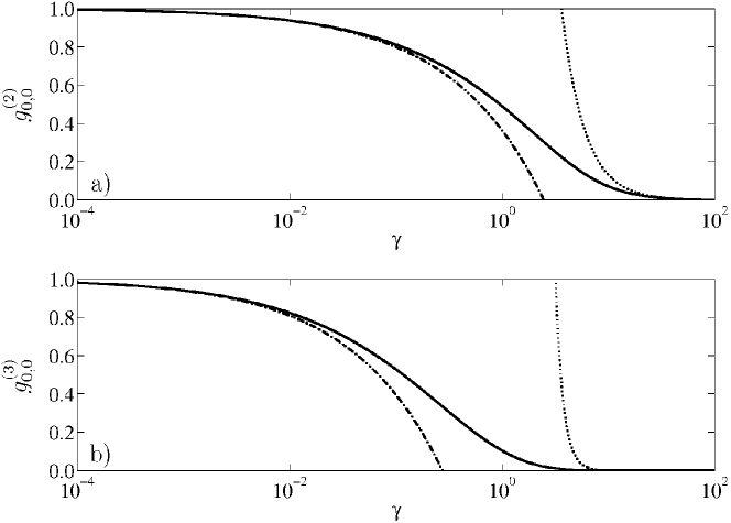
A comparison of these approximations with the exact solution is presented in figure 1. The validity of these results has recently been tested experimentally over a wide range of the correlation parameter Weiss05 and will be used to probe the extended mean-field approach presented in the next section.
Refer to caption
Figure 1: The Lieb-Liniger correlation function versus the correlation parameter γ𝛾\gamma. In subplot a), we depict the second order correlator gLL(2)subscriptsuperscript𝑔2𝐿𝐿g^{(2)}_{LL} (solid line), the Gross-Pitaevskii approximation gLL,GP(2)subscriptsuperscript𝑔2𝐿𝐿𝐺𝑃g^{(2)}_{{LL,GP}} (dashed dotted line) and the Tonks-Girardeau approximation gLL,TG(2)subscriptsuperscript𝑔2𝐿𝐿𝑇𝐺g^{(2)}_{{LL,TG}} (dotted line), while subplot b) shows the third order correlator gLL(3)subscriptsuperscript𝑔3𝐿𝐿g^{(3)}_{{LL}} (solid line) and the approximations gLL,GP(3)subscriptsuperscript𝑔3𝐿𝐿𝐺𝑃g^{(3)}_{{LL,GP}} (dashed dotted line) and gLL,TG(3)subscriptsuperscript𝑔3𝐿𝐿𝑇𝐺g^{(3)}_{{LL,TG}} (dotted line).

It is also possible to derive an exact result for the diagonal part of the third order correlation function within the framework of Lieb-Liniger theory, however the task is considerably more difficult. The exact result is derived in Cheianov2006b by introducing a new function e~(γ)~𝑒𝛾\tilde{e}(\gamma) which has the form

e~(γ)~𝑒𝛾\displaystyle\tilde{e}(\gamma) =\displaystyle= γ5λ5(γ)11dxh(x,γ)x4superscript𝛾5superscript𝜆5𝛾superscriptsubscript11differential-d𝑥𝑥𝛾superscript𝑥4\displaystyle\frac{\gamma^{5}}{\lambda^{5}(\gamma)}\int_{-1}^{1}{\rm d}x\,h(x,\gamma)x^{4} (10)

and with the help of this function one obtains

gLL(3)subscriptsuperscript𝑔3𝐿𝐿\displaystyle g^{(3)}_{{LL}} =\displaystyle= 3e~(γ)4e(γ)6e(γ)e(γ)2γ+(1+γ2)e(γ)+9e2(γ)5e~(γ)γ2.3superscript~𝑒𝛾4𝑒𝛾6𝑒𝛾superscript𝑒𝛾2𝛾1𝛾2superscript𝑒𝛾9superscript𝑒2𝛾5~𝑒𝛾superscript𝛾2\displaystyle\frac{3\tilde{e}^{\prime}(\gamma)-4e(\gamma)-6e(\gamma)e^{\prime}(\gamma)}{2\gamma}+\left(1+\frac{\gamma}{2}\right)e^{\prime}(\gamma)+\frac{9{e}^{2}(\gamma)-5\tilde{e}(\gamma)}{\gamma^{2}}. (11)

A comparison of the exact result for the third order correlation function with the approximations in the Gross-Pitaevskii and the Tonks-Girardeau regime Shlyap03 is presented in figure 1

gLL,GP(3)=16γπ, for γ1,gLL,TG(3)=16π615γ6, for γ1.formulae-sequencesubscriptsuperscript𝑔3𝐿𝐿𝐺𝑃16𝛾𝜋formulae-sequencemuch-less-than for 𝛾1formulae-sequencesubscriptsuperscript𝑔3𝐿𝐿𝑇𝐺16superscript𝜋615superscript𝛾6much-greater-than for 𝛾1g^{(3)}_{{LL,GP}}=1-\frac{6\sqrt{\gamma}}{\pi},\mbox{ for }\gamma\ll 1,\qquad g^{(3)}_{{LL,TG}}=\frac{16\pi^{6}}{15\gamma^{6}},\mbox{ for }\gamma\gg 1. (12)

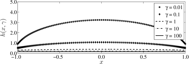
The auxiliary function h(x,γ)𝑥𝛾h(x,\gamma) of (8) is depicted for various values of the correlation parameter in figure 2.
Refer to caption
Figure 2: The auxiliary Lieb-Liniger function h(x,γ)𝑥𝛾h(x,\gamma), as a function of the variable x𝑥x for five different values of the correlation parameter γ𝛾\gamma.

III Extended mean-field theory for bosons in one dimension

III.1 Time-dependent Hartree-Fock-Bogoliubov equations

The evolution of a weakly interacting dilute gas of bosons in three dimensions can be described by a Hamiltonian

H^^𝐻\displaystyle\hat{H} =\displaystyle= d6xya^𝐱[𝐱𝐲+12Vbin(𝐱𝐲)a^𝐲a^𝐲]a^𝐱,superscriptd6𝑥𝑦subscriptsuperscript^𝑎𝐱delimited-[]subscriptsuperscriptabsent𝐱𝐲12subscript𝑉𝑏𝑖𝑛𝐱𝐲subscriptsuperscript^𝑎𝐲subscriptsuperscript^𝑎absent𝐲subscriptsuperscript^𝑎absent𝐱\displaystyle\int{\rm d}^{6}xy\,\hat{a}^{\dagger}_{\mathbf{x}}\left[\mathcal{H}^{\phantom{\dagger}}_{\mathbf{xy}}+\frac{1}{2}V_{bin}(\mathbf{x}-\mathbf{y})\hat{a}^{\dagger}_{\mathbf{y}}\hat{a}^{\phantom{\dagger}}_{\mathbf{y}}\right]\hat{a}^{\phantom{\dagger}}_{\mathbf{x}}, (13)
𝐱𝐲subscript𝐱𝐲\displaystyle\mathcal{H}_{\mathbf{xy}} =\displaystyle= 𝐱|𝐩22m+Vext(𝐱)|𝐲,Vext(𝐱)=12mω2x2+12mω2(y2+z2),quantum-operator-product𝐱superscript𝐩22𝑚subscript𝑉𝑒𝑥𝑡𝐱𝐲subscript𝑉𝑒𝑥𝑡𝐱12𝑚superscript𝜔2superscript𝑥212𝑚superscriptsubscript𝜔perpendicular-to2superscript𝑦2superscript𝑧2\displaystyle\langle\mathbf{x}|\frac{\mathbf{p}^{2}}{2m}+V_{ext}(\mathbf{x})|\mathbf{y}\rangle,\quad V_{ext}(\mathbf{x})=\frac{1}{2}m\omega^{2}x^{2}+\frac{1}{2}m\omega_{\perp}^{2}(y^{2}+z^{2}), (14)

where \mathcal{H} is the single-particle energy in an external potential Vextsubscript𝑉𝑒𝑥𝑡V_{ext} and Vbinsubscript𝑉𝑏𝑖𝑛V_{bin} is the two-particle potential. As we are interested in the quasi one-dimensional limit, we will consider a cigar shaped trapping configuration (angular frequencies ω𝜔\omega and ωsubscript𝜔perpendicular-to\omega_{\perp}) with a large aspect ratio β𝛽\beta. The energy and length scales will be set by the transverse oscillator

β=ω/ω1,a=/mω,ε=ω.formulae-sequence𝛽subscript𝜔perpendicular-to𝜔much-greater-than1formulae-sequencesubscript𝑎perpendicular-toPlanck-constant-over-2-pi𝑚subscript𝜔perpendicular-tosubscript𝜀perpendicular-toPlanck-constant-over-2-pisubscript𝜔perpendicular-to\beta=\omega_{\perp}/\omega\gg 1,\quad a_{\perp}=\sqrt{\hbar/m\omega_{\perp}},\quad\varepsilon_{\perp}=\hbar\omega_{\perp}. (15)

Conceptually, it is straight forward in the extended mean-field theory to use real, finite range binary interaction potentials and obtain proper two-body T matrices including many-body corrections. However, for convenience, we will use the pseudo-potential approximation in here

Vbin(𝐱𝐲)=4π2asmδ𝐱𝐲,subscript𝑉𝑏𝑖𝑛𝐱𝐲4𝜋superscriptPlanck-constant-over-2-pi2subscript𝑎𝑠𝑚subscript𝛿𝐱𝐲V_{bin}(\mathbf{x}-\mathbf{y})=\frac{4\pi\hbar^{2}a_{s}}{m}\delta_{\mathbf{x-y}}, (16)

where assubscript𝑎𝑠a_{s} denotes the s-wave scattering length. In order to compactify the notation we will interchangeably use a subscript notation also for continuous functions.

Extended mean-field theory uses a reduced state description based on a set of master variables {iI|γi}conditional-set𝑖𝐼subscript𝛾𝑖\{i\in I|\gamma_{i}\}. Basically, this implies the existence of a well separated hierarchy of time, energy and length scales peletminskii ; zubarev1 and leads to a rapid attenuation of correlation functions. Mathematically speaking, it allows for a selfconsistent expansion of the full many-body density matrix 𝝆𝝆\bm{\rho} in terms of a perturbation series of simple many-body density matrices 𝝈(i)superscript𝝈𝑖\bm{\sigma}^{(i)}, which depend parametrically on the master variables

𝝆=𝝈{γ}(0)+𝝈{γ}(1)+𝒪(Vbin2).𝝆subscriptsuperscript𝝈0𝛾subscriptsuperscript𝝈1𝛾𝒪superscriptsubscript𝑉𝑏𝑖𝑛2\bm{\rho}=\bm{\sigma}^{(0)}_{\{\gamma\}}+\bm{\sigma}^{(1)}_{\{\gamma\}}+\mathcal{O}(V_{bin}^{2}). (17)

This non-perturbative series in terms of the interaction potential Vbinsubscript𝑉𝑏𝑖𝑛V_{bin} has been introduced first by Chapman and Enskog in the context of kinetic theory of gases chapman . In addition to the simple series expansion, we impose a selfconsistency constraint such that the operators γ^isubscript^𝛾𝑖\hat{\gamma}_{i}, corresponding to the c-number master variables γisubscript𝛾𝑖\gamma_{i}, fulfill

γi=γ^i=Tr[γ^i𝝆]=Tr[γ^i𝝈{γ}(0)].subscript𝛾𝑖delimited-⟨⟩subscript^𝛾𝑖Trdelimited-[]subscript^𝛾𝑖𝝆Trdelimited-[]subscript^𝛾𝑖subscriptsuperscript𝝈0𝛾\gamma_{i}=\langle{\hat{\gamma}_{i}}\rangle={\rm Tr}[\hat{\gamma}_{i}\bm{\rho}]={\rm Tr}[\hat{\gamma}_{i}\bm{\sigma}^{(0)}_{\{\gamma\}}]. (18)

As far as the master variables are concerned, we choose the mean-field α𝐱subscriptsuperscript𝛼absent𝐱\alpha^{\phantom{\dagger}}_{\mathbf{x}}, the normal fluctuations of the single-particle density f~~𝑓\tilde{f} and the fluctuations of the anomalous two-particle correlation function m~~𝑚\tilde{m} such that

a^𝐱=α𝐱f𝐱,𝐲(c)=α𝐱α𝐲,m𝐱,𝐲(c)=α𝐱α𝐲,formulae-sequencedelimited-⟨⟩subscriptsuperscript^𝑎absent𝐱subscriptsuperscript𝛼absent𝐱formulae-sequencesubscriptsuperscript𝑓𝑐𝐱𝐲subscriptsuperscript𝛼absent𝐱subscriptsuperscript𝛼𝐲subscriptsuperscript𝑚𝑐𝐱𝐲subscriptsuperscript𝛼absent𝐱subscriptsuperscript𝛼absent𝐲\displaystyle\langle\hat{a}^{\phantom{\dagger}}_{\mathbf{x}}\rangle=\alpha^{\phantom{\dagger}}_{\mathbf{x}}\quad f^{(c)}_{\mathbf{x},\mathbf{y}}=\alpha^{\phantom{\dagger}}_{\mathbf{x}}\alpha^{*}_{\mathbf{y}},\quad m^{(c)}_{\mathbf{x},\mathbf{y}}=\alpha^{\phantom{\dagger}}_{\mathbf{x}}\alpha^{\phantom{\dagger}}_{\mathbf{y}}, (19)
a^𝐲a^𝐱=f𝐱,𝐲(c)+f~𝐱,𝐲,a^𝐲a^𝐱=m𝐱,𝐲(c)+m~𝐱,𝐲.formulae-sequencedelimited-⟨⟩subscriptsuperscript^𝑎𝐲subscriptsuperscript^𝑎absent𝐱subscriptsuperscript𝑓𝑐𝐱𝐲subscriptsuperscript~𝑓absent𝐱𝐲delimited-⟨⟩subscriptsuperscript^𝑎absent𝐲subscriptsuperscript^𝑎absent𝐱subscriptsuperscript𝑚𝑐𝐱𝐲subscriptsuperscript~𝑚absent𝐱𝐲\displaystyle\langle\hat{a}^{\dagger}_{\mathbf{y}}\hat{a}^{\phantom{\dagger}}_{\mathbf{x}}\rangle=f^{(c)}_{\mathbf{x},\mathbf{y}}+\tilde{f}^{\phantom{\dagger}}_{\mathbf{x},\mathbf{y}},\quad\langle\hat{a}^{\phantom{\dagger}}_{\mathbf{y}}\hat{a}^{\phantom{\dagger}}_{\mathbf{x}}\rangle=m^{(c)}_{\mathbf{x},\mathbf{y}}+\tilde{m}^{\phantom{\dagger}}_{\mathbf{x},\mathbf{y}}. (20)

A Gaussian operator 𝝈{γ}(0)subscriptsuperscript𝝈0𝛾\bm{\sigma}^{(0)}_{\{\gamma\}} is compatible with the requirements of (18,19,20). In turn, this implies the factorizability of multi operator products (Wick’s theorem) and also yields non-Gaussian corrections by calculating the contribution of 𝝈{γ}(1)subscriptsuperscript𝝈1𝛾\bm{\sigma}^{(1)}_{\{\gamma\}}.

By studying the coordinate transformation properties of the fluctuations Blaizot_ , one finds that the averages f~~𝑓\tilde{f} and m~~𝑚\tilde{m} are components of a positive semi-definite, generalized density matrix G0𝐺0G\geq 0 . Thus, the system is described by a row vector χ𝜒\chi, containing the mean-field α𝛼\alpha as well as its complex conjugate, and by the density matrix G𝐺G

χ𝐱=(α𝐱α𝐱),G𝐱,𝐲=(f~𝐱,𝐲m~𝐱,𝐲m~𝐱,𝐲δ𝐱,𝐲+f~𝐱,𝐲).formulae-sequencesubscriptsuperscript𝜒absent𝐱subscriptsuperscript𝛼absent𝐱subscriptsuperscript𝛼𝐱subscript𝐺𝐱𝐲subscriptsuperscript~𝑓absent𝐱𝐲subscriptsuperscript~𝑚absent𝐱𝐲subscriptsuperscript~𝑚𝐱𝐲subscript𝛿𝐱𝐲subscriptsuperscript~𝑓𝐱𝐲\chi^{\phantom{\dagger}}_{\bf{x}}=\left(\begin{array}[]{c}\alpha^{\phantom{*}}_{\mathbf{x}}\\ \alpha^{*}_{\mathbf{x}}\end{array}\right),\quad G_{\mathbf{x,y}}=\left(\begin{array}[]{cc}\tilde{f}^{\phantom{\dagger}}_{\mathbf{x,y}}&\tilde{m}^{\phantom{\dagger}}_{\mathbf{x,y}}\\ \tilde{m}^{\phantom{\dagger}*}_{\mathbf{x,y}}&\delta_{\mathbf{x},\mathbf{y}}+\tilde{f}^{\phantom{\dagger}*}_{\mathbf{x,y}}\end{array}\right). (21)

It can be shown from a Cauchy-Schwartz inequality that at T=0𝑇0T=0, the generalized density matrix G𝐺G obeys an idem-potency relation

Gσ3G+G=0,σ3=(𝟙00𝟙).formulae-sequence𝐺subscript𝜎3𝐺𝐺0subscript𝜎31001G\sigma_{3}G+G=0,\quad\sigma_{3}=\left(\begin{array}[]{cc}\mathds{1}&\phantom{-}0\\ 0&-\mathds{1}\end{array}\right). (22)

Starting with the Heisenberg equation of motion, it is straightforward to derive the equations of motion for χ𝜒\chi and G𝐺G. In order to obtain higher-order correlation functions within the present approximation scheme Walser99 ; Walser01 , like g(2)superscript𝑔2g^{(2)} or g(3)superscript𝑔3g^{(3)} of (1,2), one has to evaluate the Gaussian Tr[𝝈{γ}(0)]Trdelimited-[]subscriptsuperscript𝝈0𝛾{\rm Tr}[\ldots\bm{\sigma}^{(0)}_{\{\gamma\}}] as well as the non-Gaussian contributions Tr[𝝈{γ}(1)]Trdelimited-[]subscriptsuperscript𝝈1𝛾{\rm Tr}[\ldots\bm{\sigma}^{(1)}_{\{\gamma\}}]. However it is clear that the Gaussian contribution will dominate for weak correlations. Thus, we have evaluated in here only the Gaussian contributions. But already for γ1𝛾1\gamma\approx 1, deviations from that can be noticed.

III.2 Reduction to a quasi one-dimensional, stationary configuration

In a very prolate trap, the transverse motion in the directions y𝑦y and z𝑧z is effectively frozen out and only amplitudes proportional to the ground state

φ0(y,z,t)=e(y2+z2)/2a2iωtπasubscript𝜑0𝑦𝑧𝑡superscript𝑒superscript𝑦2superscript𝑧22subscriptsuperscript𝑎2perpendicular-to𝑖subscript𝜔perpendicular-to𝑡𝜋subscript𝑎perpendicular-to\varphi_{0}(y,z,t)=\frac{e^{-(y^{2}+z^{2})/2a^{2}_{\perp}-i\omega_{\perp}t}}{\sqrt{\pi}a_{\perp}} (23)

need to be considered. By projecting all three-dimensional functions onto the longitudinal axis 𝐱x𝐱𝑥\mathbf{x}\rightarrow x, one obtains the time-dependent Hartree-Fock-Bogoliubov equations (THFB) for χxsubscript𝜒𝑥\chi_{x} and Gx,xsubscript𝐺𝑥superscript𝑥G_{x,x^{\prime}}

itχx=Πxχx+𝒪(Vbin2),itGx,x=ΣxGx,xh. c.+𝒪(Vbin2),formulae-sequence𝑖Planck-constant-over-2-pisubscript𝑡subscript𝜒𝑥subscriptΠ𝑥subscript𝜒𝑥𝒪superscriptsubscript𝑉𝑏𝑖𝑛2𝑖Planck-constant-over-2-pisubscript𝑡subscript𝐺𝑥superscript𝑥subscriptsuperscriptΣabsent𝑥subscriptsuperscript𝐺absent𝑥superscript𝑥h. c.𝒪superscriptsubscript𝑉𝑏𝑖𝑛2i\hbar\partial_{t}\chi_{x}=\Pi_{x}\chi_{x}+\mathcal{O}(V_{bin}^{2}),\,\,i\hbar\partial_{t}G_{x,x^{\prime}}=\Sigma^{\phantom{\dagger}}_{x}G^{\phantom{\dagger}}_{x,x^{\prime}}-\mbox{h. c.}+\mathcal{O}(V_{bin}^{2}), (24)

with the following abbreviations for the single particle Hamiltonian and the self energies

Πx=(ΠNΠAΠAΠN),Σx=(ΣNΣAΣAΣN),formulae-sequencesubscriptΠ𝑥subscriptΠ𝑁subscriptΠ𝐴superscriptsubscriptΠ𝐴superscriptsubscriptΠ𝑁subscriptΣ𝑥subscriptΣ𝑁subscriptΣ𝐴superscriptsubscriptΣ𝐴superscriptsubscriptΣ𝑁\displaystyle\Pi_{x}=\left(\begin{array}[]{cc}\phantom{-}\Pi_{N}&\phantom{-}\Pi_{A}\\ -\Pi_{A}^{*}&-\Pi_{N}^{*}\end{array}\right),\quad\Sigma_{x}=\left(\begin{array}[]{cc}\phantom{-}\Sigma_{N}&\phantom{-}\Sigma_{A}\\ -\Sigma_{A}^{*}&-\Sigma_{N}^{*}\\ \end{array}\right), (29)
ΠNsubscriptΠ𝑁\displaystyle\Pi_{N} =\displaystyle= x+gfx,x(c)+2gf~x,x,ΣN=x+2gfx,x(c)+2gf~x,x,subscriptsuperscriptabsent𝑥𝑔subscriptsuperscript𝑓𝑐𝑥𝑥2𝑔subscriptsuperscript~𝑓absent𝑥𝑥subscriptΣ𝑁subscriptsuperscriptabsent𝑥2𝑔subscriptsuperscript𝑓𝑐𝑥𝑥2𝑔subscriptsuperscript~𝑓absent𝑥𝑥\displaystyle\mathcal{H}^{\phantom{\dagger}}_{x}+gf^{(c)}_{x,x}+2g\tilde{f}^{\phantom{\dagger}}_{x,x},\quad\Sigma_{N}=\mathcal{H}^{\phantom{\dagger}}_{x}+2gf^{(c)}_{x,x}+2g\tilde{f}^{\phantom{\dagger}}_{x,x}, (30)
ΣAsubscriptΣ𝐴\displaystyle\Sigma_{A} =\displaystyle= gmx,x(c)+gm~x,x,ΠA=gm~x,x,x=22mx2+12β2mω2x2.formulae-sequence𝑔subscriptsuperscript𝑚𝑐𝑥𝑥𝑔subscriptsuperscript~𝑚absent𝑥𝑥subscriptΠ𝐴𝑔subscriptsuperscript~𝑚absent𝑥𝑥subscript𝑥superscriptPlanck-constant-over-2-pi22𝑚subscriptsuperscript2𝑥12superscript𝛽2𝑚superscriptsubscript𝜔perpendicular-to2superscript𝑥2\displaystyle gm^{(c)}_{x,x}+g\tilde{m}^{\phantom{\dagger}}_{x,x},\quad\Pi_{A}=g\tilde{m}^{\phantom{\dagger}}_{x,x},\quad\mathcal{H}_{x}=-\frac{\hbar^{2}}{2m}\partial^{2}_{x}+\frac{1}{2\beta^{2}}m\omega_{\perp}^{2}x^{2}. (31)

In the course of the dimensional reduction, we had to introduce an effective one-dimensional coupling constant g=2ωas𝑔2Planck-constant-over-2-pisubscript𝜔perpendicular-tosubscript𝑎𝑠g=2\hbar\omega_{\perp}{a}_{s}, which is in agreement with previous derivations walser04 ; Olshanii98 ; MenStrin02 . In order to obtain the stationary solution for the time-independent fields χxsubscript𝜒𝑥\chi_{x} and Gx,xsubscript𝐺𝑥superscript𝑥G_{x,x^{\prime}}, we make the ansatz

χ(t)=eiμtσ3χ,G(t)=eiμtσ3Geiμtσ3formulae-sequence𝜒𝑡superscript𝑒𝑖Planck-constant-over-2-pi𝜇𝑡subscript𝜎3𝜒𝐺𝑡superscript𝑒𝑖Planck-constant-over-2-pi𝜇𝑡subscript𝜎3𝐺superscript𝑒𝑖Planck-constant-over-2-pi𝜇𝑡subscript𝜎3\chi(t)=e^{-\frac{i}{\hbar}\mu t\sigma_{3}}\chi,\quad G(t)=e^{-\frac{i}{\hbar}\mu t\sigma_{3}}\,G\,e^{\frac{i}{\hbar}\mu t\sigma_{3}} (32)

which introduces the chemical potential μ𝜇\mu and employs the Pauli matrix σ3subscript𝜎3\sigma_{3} of (22). This ansatz implies that the normal fluctuations f~x,x(t)subscript~𝑓𝑥superscript𝑥𝑡\tilde{f}_{x,x^{\prime}}(t) become time-independent, while the anomalous fluctuations m~x,x(t)subscript~𝑚𝑥superscript𝑥𝑡\tilde{m}_{x,x^{\prime}}(t) oscillate with twice the chemical potential. The properties of the resulting stationary HFB equation will be investigated in section IV in the case of a homogeneous gas of bosons and in section V for a harmonic trapping potential, both at zero and for finite temperatures.

The fact that the eigenvalue in the resulting stationary equations is indeed the chemical potential Blaizot_ can be seen from a variation of the total energy functional (α,f~,m~)=H^𝛼~𝑓~𝑚delimited-⟨⟩^𝐻\mathcal{E}(\alpha,\tilde{f},\tilde{m})=\langle\hat{H}\rangle given by

\displaystyle\mathcal{E} =\displaystyle= dxdyδ(xy)[αy(x+g2|αx|2)αx+(y+gf~x,y)f~x,y]differential-d𝑥differential-d𝑦𝛿𝑥𝑦delimited-[]subscriptsuperscript𝛼𝑦subscriptsuperscriptabsent𝑥𝑔2superscriptsubscriptsuperscript𝛼absent𝑥2subscriptsuperscript𝛼absent𝑥subscriptsuperscriptabsent𝑦𝑔subscriptsuperscript~𝑓absent𝑥𝑦subscriptsuperscript~𝑓absent𝑥𝑦\displaystyle\int{\rm d}x{\rm d}y\,\delta(x-y)[\alpha^{*}_{y}(\mathcal{H}^{\phantom{\dagger}}_{{x}}+\frac{g}{2}|\alpha^{\phantom{\dagger}}_{x}|^{2})\alpha^{\phantom{\dagger}}_{x}+(\mathcal{H}^{\phantom{\dagger}}_{{y}}+g\tilde{f}^{\phantom{\dagger}}_{{x},{y}})\tilde{f}^{\phantom{\dagger}}_{{x},{y}}] (33)
+g2dx[(2|αx|2f~x,x+αx2m~x,x+12|m~x,x|2)+h. c.]+𝒪(Vbin2),𝑔2differential-d𝑥delimited-[]2superscriptsubscriptsuperscript𝛼absent𝑥2subscriptsuperscript~𝑓absent𝑥𝑥superscriptsubscript𝛼𝑥2subscriptsuperscript~𝑚𝑥𝑥12superscriptsubscriptsuperscript~𝑚absent𝑥𝑥2h. c.𝒪superscriptsubscript𝑉𝑏𝑖𝑛2\displaystyle+\frac{g}{2}\int{\rm d}x[(2|\alpha^{\phantom{\dagger}}_{x}|^{2}\tilde{f}^{\phantom{\dagger}}_{{x},{x}}+{\alpha_{x}}^{2}\tilde{m}^{*}_{{x},{x}}+\frac{1}{2}|\tilde{m}^{\phantom{\dagger}}_{{x},{x}}|^{2})+\mbox{h. c.}]+\mathcal{O}(V_{bin}^{2}),

with the constraint that the number of particles N=dx(fx,x(c)+f~x,x)𝑁differential-d𝑥subscriptsuperscript𝑓𝑐𝑥𝑥subscript~𝑓𝑥𝑥N=\int{\rm d}x(f^{(c)}_{x,x}+\tilde{f}_{{x},{x}}).

IV Analytic solution for the stationary HFB-equations in the homogeneous system at zero temperature

For the calculations that are presented in the following sections, we use standard parameters for 87Rb in natural units of length asubscript𝑎perpendicular-toa_{\perp} and energy εsubscript𝜀perpendicular-to\varepsilon_{\perp}

m=1.44321025 kg,as=5.8209109 m,ω=2π800 Hz,ω=2π3 Hz,a=3.8128107 m,g~=2as/a=3.0533102.𝑚1.4432superscript1025 kgsubscript𝑎𝑠5.8209superscript109 mmissing-subexpressionsubscript𝜔perpendicular-to2𝜋800 Hz𝜔2𝜋3 Hzmissing-subexpressionsubscript𝑎perpendicular-to3.8128superscript107 m~𝑔2subscript𝑎𝑠subscript𝑎perpendicular-to3.0533superscript102missing-subexpression\begin{array}[]{lll}m=1.4432\cdot 10^{-25}\mbox{ kg},&a_{s}=5.8209\cdot 10^{-9}\mbox{ m},\\ \omega_{\perp}=2\pi\cdot 800\mbox{ Hz},&\omega=2\pi\cdot 3\mbox{ Hz},\\ a_{\perp}=3.8128\cdot 10^{-7}\mbox{ m},&\tilde{g}=2a_{s}/a_{\perp}=3.0533\cdot 10^{-2}.\end{array} (34)

To reach the homogeneous case, we have to decrease the influence of the external trapping potential in (31) by weakening it to the limit β1much-greater-than𝛽1\beta\gg 1, where we can neglect it practically. Therefore, the equilibrium state should possess the same translation symmetry as the generator of the dynamics. Consequently, we can assume that the mean field is space independent αx=αsubscript𝛼𝑥𝛼\alpha_{x}=\alpha and the density matrix only depends on relative differences r=xx𝑟𝑥superscript𝑥r=x-x^{\prime}

χx=χ,Gx,x=Gxx=dk2πeikr𝒢k.formulae-sequencesubscript𝜒𝑥𝜒subscript𝐺𝑥superscript𝑥subscript𝐺𝑥superscript𝑥superscriptsubscriptd𝑘2𝜋superscript𝑒𝑖𝑘𝑟subscript𝒢𝑘\chi_{x}=\chi,\qquad G_{x,x^{\prime}}=G_{x-x^{\prime}}=\int_{-\infty}^{\infty}\frac{{\rm d}k}{2\pi}\,e^{-ikr}\mathcal{G}_{k}\;. (35)

Translation invariant systems are best described in Fourier-space, which was introduced above. We can also choose the mean-field to be real-valued by a suitable phase rotation. This is a consequence of the global number conservation that is built into the dynamical HFB equations Griffin96 . As the mean-field is real-valued f(c)=m(c)=α2superscript𝑓𝑐superscript𝑚𝑐superscript𝛼2f^{(c)}=m^{(c)}=\alpha^{2} , so are the fluctuations f~0=f~x,xsubscript~𝑓0subscript~𝑓𝑥𝑥\tilde{f}_{0}=\tilde{f}_{x,x} and m~0=m~x,xsubscript~𝑚0subscript~𝑚𝑥𝑥\tilde{m}_{0}=\tilde{m}_{x,x} and with these assumptions, the normalization constraint reads

n=NL=f(c)+f~0,𝑛𝑁𝐿superscript𝑓𝑐subscript~𝑓0\displaystyle n=\frac{N}{L}=f^{(c)}+\tilde{f}_{0}, (36)

where n𝑛n is the linear particle density on a length L𝐿L. Furthermore the THFB equations (24) simplify significantly to

μ=g~(f(c)+2f~0+m~0),0=(Σkμσ3)𝒢kh. c.formulae-sequence𝜇~𝑔superscript𝑓𝑐2subscript~𝑓0subscript~𝑚00subscriptΣ𝑘𝜇subscript𝜎3subscript𝒢𝑘h. c.\mu=\tilde{g}(f^{(c)}+2\tilde{f}_{0}+\tilde{m}_{0}),\qquad 0=(\Sigma_{k}-\mu\sigma_{3})\mathcal{G}_{k}-\mbox{h. c.} (37)

From the equation for the chemical potential, it is clear that energy and length scales emerge. It will be beneficial to introduce such scales for coherence (kc,ξc,ωcsubscript𝑘𝑐subscript𝜉𝑐subscript𝜔𝑐k_{c},\xi_{c},\omega_{c}), the pairing correlations (k~,ξ~,ω~~𝑘~𝜉~𝜔{\tilde{k}},{\tilde{\xi}},{\tilde{\omega}}), and their weighted sums and differences as

kc=ξc1=ωc,k~=ξ~1=ω~,k±=ξ±1=ω±formulae-sequencesubscript𝑘𝑐superscriptsubscript𝜉𝑐1subscript𝜔𝑐~𝑘superscript~𝜉1~𝜔subscript𝑘plus-or-minussuperscriptsubscript𝜉plus-or-minus1subscript𝜔plus-or-minus\displaystyle k_{c}=\xi_{c}^{-1}=\sqrt{\omega_{c}},\quad{\tilde{k}}={{\tilde{\xi}}}^{-1}=\sqrt{{\tilde{\omega}}},\quad k_{\pm}={\xi_{\pm}}^{-1}=\sqrt{\omega_{\pm}} (38)
ωc=4g~f(c),ω~=4g~m~0,ω±=ωc±ω~2.formulae-sequencesubscript𝜔𝑐4~𝑔superscript𝑓𝑐formulae-sequence~𝜔4~𝑔subscript~𝑚0subscript𝜔plus-or-minusplus-or-minussubscript𝜔𝑐~𝜔2\displaystyle\omega_{c}=4\tilde{g}f^{(c)},\qquad{\tilde{\omega}}=-4\tilde{g}\tilde{m}_{0},\qquad\omega_{\pm}=\frac{\omega_{c}\pm{\tilde{\omega}}}{2}. (39)

In particular, in the Gross-Pitaevskii regime one can assume that ωcω~much-greater-thansubscript𝜔𝑐~𝜔\omega_{c}\gg{\tilde{\omega}}. With these definitions, one finds that the self energy is simply a 2×2222\times 2 matrix in k𝑘k-space with eigenvalues ωksubscript𝜔𝑘\omega_{k}

Σkμσ3=12(k2+ω+ωωk2ω+),ωk=12(k2+ωc)(k2+ω~).formulae-sequencesubscriptΣ𝑘𝜇subscript𝜎312superscript𝑘2subscript𝜔subscript𝜔subscript𝜔superscript𝑘2subscript𝜔subscript𝜔𝑘12superscript𝑘2subscript𝜔𝑐superscript𝑘2~𝜔\Sigma_{k}-\mu\sigma_{3}=\frac{1}{2}\left(\begin{array}[]{cc}k^{2}+\omega_{+}&\omega_{-}\\ -\omega_{-}&-k^{2}-\omega_{+}\end{array}\right),\,\omega_{k}=\frac{1}{2}\sqrt{(k^{2}+\omega_{c})(k^{2}+{\tilde{\omega}})}. (40)

Now, we can finally evaluate the density matrix part of the HFB equations (37). Moreover, we also have to consider the idem-potency relation of (22). It holds for the vacuum state at zero temperature and one obtains another, now quadratic relation between normal and anomalous fluctuations in k𝑘k-space

m~k=ωk2+ω+(12+f~k),f~k=m~k2f~k2.formulae-sequencesubscript~𝑚𝑘subscript𝜔superscript𝑘2subscript𝜔12subscript~𝑓𝑘subscript~𝑓𝑘superscriptsubscript~𝑚𝑘2superscriptsubscript~𝑓𝑘2\tilde{m}_{k}=-\frac{\omega_{-}}{k^{2}+\omega_{+}}\left(\frac{1}{2}+\tilde{f}_{k}\right),\quad\tilde{f}_{k}=\tilde{m}_{k}^{2}-\tilde{f}_{k}^{2}. (41)

The system of equations can be solved point wise in k𝑘k-space and leads to two solutions. One of which has to be rejected on physical grounds. Thus, we find

m~k=ω4ωk,f~k=k2+ω+4ωk12.formulae-sequencesubscript~𝑚𝑘subscript𝜔4subscript𝜔𝑘subscript~𝑓𝑘superscript𝑘2subscript𝜔4subscript𝜔𝑘12\tilde{m}_{k}=-\frac{\omega_{-}}{4\omega_{k}},\quad\tilde{f}_{k}=\frac{k^{2}+\omega_{+}}{4\omega_{k}}-\frac{1}{2}. (42)

The high momentum tail of the correlation functions is responsible for the short scale behaviour in real space. In the limit k𝑘k\to\infty the leading terms are

m~kω2k2,f~km~k2.formulae-sequencesimilar-tosubscript~𝑚𝑘subscript𝜔2superscript𝑘2similar-tosubscript~𝑓𝑘superscriptsubscript~𝑚𝑘2\tilde{m}_{k}\sim-\frac{\omega_{-}}{2k^{2}},\quad\tilde{f}_{k}\sim\tilde{m}_{k}^{2}. (43)

IV.1 Diagonal contributions of normal and anomalous fluctuations

In order to obtain the diagonal part of the translation invariant correlation functions m~rsubscript~𝑚𝑟\tilde{m}_{r} and f~rsubscript~𝑓𝑟\tilde{f}_{r} at r=0𝑟0r=0, we have to evaluate the inverse Fourier transform of (35)

m~0=ω8πdkωk,f~0=dk2πf~k.formulae-sequencesubscript~𝑚0subscript𝜔8𝜋superscriptsubscript𝑑𝑘subscript𝜔𝑘subscript~𝑓0superscriptsubscript𝑑𝑘2𝜋subscript~𝑓𝑘\tilde{m}_{0}=-\frac{\omega_{-}}{8\pi}\int_{-\infty}^{\infty}\frac{dk}{\omega_{k}},\quad\tilde{f}_{0}=\int_{-\infty}^{\infty}\frac{dk}{2\pi}\tilde{f}_{k}. (44)

Serendipitously, this can be done exactly in terms of elliptic integrals Abramowitz

m~0subscript~𝑚0\displaystyle\tilde{m}_{0} =\displaystyle= kc4π(1+m~0f(c))K(1+m~0f(c)),subscript𝑘𝑐4𝜋1subscript~𝑚0superscript𝑓𝑐𝐾1subscript~𝑚0superscript𝑓𝑐\displaystyle-\frac{k_{c}}{4\pi}\left(1+\frac{\tilde{m}_{0}}{f^{(c)}}\right)K\left(1+\frac{\tilde{m}_{0}}{f^{(c)}}\right), (45)
f~0subscript~𝑓0\displaystyle\tilde{f}_{0} =\displaystyle= m~0kc2π[E(1+m~0f(c))K(1+m~0f(c))],subscript~𝑚0subscript𝑘𝑐2𝜋delimited-[]𝐸1subscript~𝑚0superscript𝑓𝑐𝐾1subscript~𝑚0superscript𝑓𝑐\displaystyle\tilde{m}_{0}-\frac{k_{c}}{2\pi}\left[E\left(1+\frac{\tilde{m}_{0}}{f^{(c)}}\right)-K\left(1+\frac{\tilde{m}_{0}}{f^{(c)}}\right)\right], (46)

where K𝐾K and E𝐸E are the complete elliptic integral of the first kind and second kind, respectively. Basic definitions are given in A.1.

The scaling properties of the correlation functions are most relevant for a physical insight. Thus, we can study the Gross-Pitaevskii regime of weakly correlated bosons, where |m~0/f(c)|1much-less-thansubscript~𝑚0superscript𝑓𝑐1|{\tilde{m}_{0}}/{f^{(c)}}|\ll 1 and use a series expansion for the elliptic integral (1x)K(1x)ln(4/x)1𝑥𝐾1𝑥4𝑥(1-x)K(1-x)\approx\ln(4/\sqrt{x}). With this approximation we get

m~0subscript~𝑚0\displaystyle\tilde{m}_{0} =\displaystyle= g~f(c)4πW(64πf(c)/g~),f~0=g~f(c)πm~0.~𝑔superscript𝑓𝑐4𝜋𝑊64𝜋superscript𝑓𝑐~𝑔subscript~𝑓0~𝑔superscript𝑓𝑐𝜋subscript~𝑚0\displaystyle-\frac{\sqrt{\tilde{g}f^{(c)}}}{4\pi}W\left(64\pi\sqrt{f^{(c)}/\tilde{g}}\right),\quad\tilde{f}_{0}=-\frac{\sqrt{\tilde{g}f^{(c)}}}{\pi}-\tilde{m}_{0}. (47)

In this explicit formula, we had to introduce the Lambert-W𝑊W-function, which is defined in A.2 and an excellent asymptotic expansion is given in terms of logarithms knuth96 .

The approximations for the fluctuations are compared to exact numerical calculations in figure 3 and give a good agreement. We will use these approximations in the following sections to evaluate the ground state energy and correlation functions.

Refer to caption
Figure 3: Diagonal part of the anomalous fluctuations m~0subscript~𝑚0-\tilde{m}_{0} (left scale, solid line) and normal fluctuations f~0subscript~𝑓0\tilde{f}_{0} (right scale, dashed line) versus mean field density f(c)superscript𝑓𝑐f^{(c)}. The asymptotic approximations for m~0subscript~𝑚0\tilde{m}_{0} (dashed dotted line) and f~0subscript~𝑓0\tilde{f}_{0} (dotted line) according to (47) agree well for the considered parameter range.

IV.2 Off-diagonal contribution of normal and anomalous fluctuations

IV.2.1 Short length scale behaviour: rξ~much-less-than𝑟~𝜉r\ll{\tilde{\xi}}

A rather simple, yet surprisingly efficient insight into the short range behaviour of the off-diagonal of the fluctuations can be obtained by using an iteration scheme for their Fourier transforms, which has its origin in (41). Starting with f~k(0)=0superscriptsubscript~𝑓𝑘00\tilde{f}_{k}^{(0)}=0 and using the recursion relation

m~k(i+1)superscriptsubscript~𝑚𝑘𝑖1\displaystyle\tilde{m}_{k}^{(i+1)} =\displaystyle= ωk2+ω+(12+f~k(i)),f~k(i+1)=(m~k(i+1))2(f~k(i))2subscript𝜔superscript𝑘2subscript𝜔12superscriptsubscript~𝑓𝑘𝑖superscriptsubscript~𝑓𝑘𝑖1superscriptsuperscriptsubscript~𝑚𝑘𝑖12superscriptsuperscriptsubscript~𝑓𝑘𝑖2\displaystyle-\frac{\omega_{-}}{k^{2}+\omega_{+}}\left(\frac{1}{2}+\tilde{f}_{k}^{(i)}\right),\quad\tilde{f}_{k}^{(i+1)}=(\tilde{m}_{k}^{(i+1)})^{2}-(\tilde{f}_{k}^{(i)})^{2} (48)

we get a rapid convergence towards the exact results. It is remarkable that even with the inverse Fourier transforms of low orders of this iteration scheme, we get a functional behaviour for f~(r)~𝑓𝑟\tilde{f}(r) and m~(r)~𝑚𝑟\tilde{m}(r), which is equivalent to their exact behaviour for short ranges. However in contrast to the exact form of the Fourier transforms of the fluctuations in (42), it is possible to perform the inverse Fourier transform analytically in every order of the iteration scheme. A closer look reveals that the dependence of the fluctuations on r𝑟r has to be of the form

m~(i)(r)superscript~𝑚𝑖𝑟\displaystyle\tilde{m}^{(i)}(r) =\displaystyle= ek+|r|P(i)(r),f~(i)(r)=ek+|r|Q(i)(r)superscript𝑒subscript𝑘𝑟superscript𝑃𝑖𝑟superscript~𝑓𝑖𝑟superscript𝑒subscript𝑘𝑟superscript𝑄𝑖𝑟\displaystyle e^{-k_{+}|r|}P^{(i)}(r),\quad\tilde{f}^{(i)}(r)=e^{-k_{+}|r|}Q^{(i)}(r) (49)

where P(i)(r)superscript𝑃𝑖𝑟P^{(i)}(r) and Q(i)(r)superscript𝑄𝑖𝑟Q^{(i)}(r) are polynomials in r𝑟r of order 2i2superscript2𝑖22^{i}-2 and 2i+13superscript2𝑖132^{i+1}-3 respectively. Consequently the length scale on which the correlations decay is given by

ξ+subscript𝜉\displaystyle\xi_{+} =\displaystyle= 1k+=12g~(f(c)m~0).1subscript𝑘12~𝑔superscript𝑓𝑐subscript~𝑚0\displaystyle\frac{1}{k_{+}}=\frac{1}{\sqrt{2\tilde{g}(f^{(c)}-\tilde{m}_{0})}}. (50)

In the Gross-Pitaevskii regime, where f(c)m~0much-greater-thansuperscript𝑓𝑐subscript~𝑚0f^{(c)}\gg\tilde{m}_{0}, we recover the healing length ξ1/2g~f(c)𝜉12~𝑔superscript𝑓𝑐\xi\approx 1/\sqrt{2\tilde{g}f^{(c)}}, already introduced at the beginning in (5).
Refer to caption
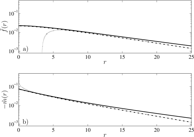
Figure 4: Off-diagonal part of the normal and anomalous fluctuations versus the distance r𝑟r. In subplot a) we depict the normal fluctuation f~(r)~𝑓𝑟\tilde{f}(r) (solid line), its short range approximation f~(4)(r)superscript~𝑓4𝑟\tilde{f}^{(4)}(r) (dashed dotted line) and the long range approximation (dotted line) according to (55). Subplot b) shows the anomalous fluctuation m~(r)~𝑚𝑟-\tilde{m}(r) (solid line), the short range approximation m~(4)(r)superscript~𝑚4𝑟-\tilde{m}^{(4)}(r) thereof (dashed dotted line) and the long range approximation (dotted line) according to (54).

The short range behaviour of the anomalous fluctuation and the normal fluctuation is depicted in figure 4. There, we compare the 4th4𝑡4th order result of the iteration scheme to the exact numerical evaluation of the inverse Fourier transform. We assumed N=100𝑁100N=100 particles, distributed over a length of L=90a𝐿90subscript𝑎perpendicular-toL=90a_{\perp}. This length was chosen such that the density in the homogeneous case is similar to the density in the center of the trapped system, which will be discussed in section V. One obtains a good agreement between the approximation and the exact results in the regime where rξ~10.5much-less-than𝑟~𝜉10.5r\ll{\tilde{\xi}}\approx 10.5 with ξ3.88𝜉3.88\xi\approx 3.88. At the origin we note that the anomalous fluctuation shows the typical cusp whereas the normal fluctuation has a smooth behaviour and consequently a vanishing first derivative at r=0𝑟0r=0.

IV.2.2 Long length scale behaviour: rξ~much-greater-than𝑟~𝜉r\gg{\tilde{\xi}}

In order to get an approximation for the fluctuations in this regime, we start with the Fourier transform of the anomalous fluctuation in (42) and note for further consideration that the Fourier transform of the modified Bessel function of the second kind K0(c|r|)subscript𝐾0𝑐𝑟K_{0}(c|r|) is given by π/k2+c2𝜋superscript𝑘2superscript𝑐2{\pi}/{\sqrt{k^{2}+c^{2}}}. Thus the convolution property of the Fourier transform yields

m~(r)~𝑚𝑟\displaystyle\tilde{m}(r) =\displaystyle= ω2π2K0(kc|r|)K0(k~|r+r|)𝑑r.subscript𝜔2superscript𝜋2superscriptsubscriptsubscript𝐾0subscript𝑘𝑐superscript𝑟subscript𝐾0~𝑘superscript𝑟𝑟differential-dsuperscript𝑟\displaystyle-\frac{\omega_{-}}{2\pi^{2}}\int_{-\infty}^{\infty}K_{0}(k_{c}|r^{\prime}|)K_{0}({\tilde{k}}|r^{\prime}\!+r|)dr^{\prime}.

The modified Bessel function of the second kind K0(r)subscript𝐾0𝑟K_{0}(r) is presented in figure 5. K0(r)subscript𝐾0𝑟K_{0}(r) diverges logarithmically at the origin and decreases exponentially for large arguments

K0(r){γe+ln2r+𝒪(r2),r0er[π2r+𝒪(r3/2)],rsimilar-tosubscript𝐾0𝑟casessubscript𝛾𝑒2𝑟𝒪superscript𝑟2𝑟0superscript𝑒𝑟delimited-[]𝜋2𝑟𝒪superscript𝑟32𝑟\displaystyle K_{0}(r)\sim\left\{\begin{array}[]{ll}-\gamma_{e}+\ln\frac{2}{r}+\mathcal{O}(r^{2}),&r\rightarrow 0\\ e^{-r}\left[\sqrt{\frac{\pi}{2r}}+\mathcal{O}(r^{-3/2})\right],&r\to\infty\end{array}\right. (53)

where γe0.5772subscript𝛾𝑒0.5772\gamma_{e}\approx 0.5772 denotes Euler’s constant.

Refer to caption
Figure 5: The modified Bessel function of the second kind K0(r)subscript𝐾0𝑟K_{0}(r) versus r𝑟r.

In the Gross-Pitaevskii regime where f(c)|m~0|much-greater-thansuperscript𝑓𝑐subscript~𝑚0{f^{(c)}}\gg|{\tilde{m}_{0}}|, we get from rξ~much-greater-than𝑟~𝜉r\gg{\tilde{\xi}} that also rξcmuch-greater-than𝑟subscript𝜉𝑐r\gg\xi_{c} and therefore the first Bessel function in the integral closely resembles a δ𝛿\delta-function. Thus we obtain the result

m~(r)~𝑚𝑟\displaystyle{\tilde{m}}(r) =\displaystyle= kc4π(1+m~0f(c))K0(k~|r|)kc4πK0(k~|r|),subscript𝑘𝑐4𝜋1subscript~𝑚0superscript𝑓𝑐subscript𝐾0~𝑘𝑟subscript𝑘𝑐4𝜋subscript𝐾0~𝑘𝑟\displaystyle-\frac{k_{c}}{4\pi}\left(1+\frac{\tilde{m}_{0}}{f^{(c)}}\right)\;K_{0}\left({\tilde{k}}|r|\right)\approx-\frac{k_{c}}{4\pi}\;K_{0}\left({\tilde{k}}|r|\right), (54)
f~(r)~𝑓𝑟\displaystyle{\tilde{f}}(r) =\displaystyle= kc8πk2[kc2K0(k~|r|)k~2K2(k~|r|)].subscript𝑘𝑐8𝜋superscriptsubscript𝑘2delimited-[]superscriptsubscript𝑘𝑐2subscript𝐾0~𝑘𝑟superscript~𝑘2subscript𝐾2~𝑘𝑟\displaystyle\frac{k_{c}}{8\pi k_{-}^{2}}[k_{c}^{2}K_{0}({\tilde{k}}|r|)-{\tilde{k}}^{2}K_{2}({\tilde{k}}|r|)]\;. (55)

An alternative derivation of this result with the help of complex integration is given in B. In figure 4 the asymptotic form of the fluctuations in terms of the Bessel functions is compared to an exact numerical simulation with the parameters that were mentioned in the previous subsection. In either case the semi-logarithmic plot reveals an exponential decay for large distances rξ~much-greater-than𝑟~𝜉r\gg{\tilde{\xi}}, in agreement with the asymptotic behaviour of the Bessel functions.

IV.3 Comparison to Lieb-Liniger theory

Having all the ingredients at hand to calculate correlation functions, we are now ready for a quantitative comparison with the results of Lieb-Liniger theory which provides an exact solution for the behaviour of the second and third order correlation function.

As outlined in section III.1, we have to obtain the values of the correlation functions from multiple operator averages. If o^^𝑜\hat{o} is such a general operator then

o^=Tr[o^(𝝈{γ}(0)+𝝈{γ}(1)+𝒪(g~2))]delimited-⟨⟩^𝑜Trdelimited-[]^𝑜subscriptsuperscript𝝈0𝛾subscriptsuperscript𝝈1𝛾𝒪superscript~𝑔2\langle\hat{o}\rangle={\rm Tr}[\hat{o}\,(\bm{\sigma}^{(0)}_{\{\gamma\}}+\bm{\sigma}^{(1)}_{\{\gamma\}}+\mathcal{O}(\tilde{g}^{2}))] (56)

While we have already evaluated the Gaussian and non-Gaussian averages for the multinomial operator averages Walser99 , it is clear that the Gaussian contribution will dominate for weak correlations.

Therefore we will focus in here on the Gaussian contribution and disregard the non-Gaussian contributions in the following explicit expressions of order two and one, respectively

gx,y(1)subscriptsuperscript𝑔1𝑥𝑦\displaystyle g^{(1)}_{x,y} =\displaystyle= fx,y(c)+f~x,ynxny+𝒪(g~2),subscriptsuperscript𝑓𝑐𝑥𝑦subscript~𝑓𝑥𝑦subscript𝑛𝑥subscript𝑛𝑦𝒪superscript~𝑔2\displaystyle\frac{f^{(c)}_{{x},{y}}+\tilde{f}_{{x},{y}}}{\sqrt{n_{x}\,n_{y}}}+\mathcal{O}(\tilde{g}^{2}), (57)
gx,y(2)subscriptsuperscript𝑔2𝑥𝑦\displaystyle g^{(2)}_{x,y} =\displaystyle= 1+2(fx,y(c)f~y,x+mx,y(c)m~y,x)+f~x,yf~y,x+m~x,ym~y,xnxny+𝒪(g~),12subscriptsuperscript𝑓𝑐𝑥𝑦subscriptsuperscript~𝑓absent𝑦𝑥superscriptsubscriptsuperscript𝑚𝑐𝑥𝑦subscriptsuperscript~𝑚absent𝑦𝑥subscriptsuperscript~𝑓absent𝑥𝑦subscriptsuperscript~𝑓absent𝑦𝑥subscriptsuperscript~𝑚absent𝑥𝑦subscriptsuperscript~𝑚𝑦𝑥subscript𝑛𝑥subscript𝑛𝑦𝒪~𝑔\displaystyle 1+\frac{2\Re(f^{(c)}_{{x},{y}}\tilde{f}^{\phantom{*}}_{{y},{x}}+{m^{(c)}_{{x},{y}}}^{*}\tilde{m}^{\phantom{*}}_{{y},{x}})+\tilde{f}^{\phantom{*}}_{{x},{y}}\tilde{f}^{\phantom{*}}_{{y},{x}}+\tilde{m}^{\phantom{*}}_{{x},{y}}{\tilde{m}^{*}_{{y},{x}}}}{n_{x}\,n_{y}}+\mathcal{O}(\tilde{g}), (58)
gx,y(3)subscriptsuperscript𝑔3𝑥𝑦\displaystyle g^{(3)}_{x,y} =\displaystyle= 1+2nxny[2(fx,y(c)f~y,x+mx,y(c)m~y,x)+f~x,yf~y,x+m~x,ym~y,x]12subscript𝑛𝑥subscript𝑛𝑦delimited-[]2subscriptsuperscript𝑓𝑐𝑥𝑦subscriptsuperscript~𝑓absent𝑦𝑥superscriptsubscriptsuperscript𝑚𝑐𝑥𝑦subscriptsuperscript~𝑚absent𝑦𝑥subscriptsuperscript~𝑓absent𝑥𝑦subscriptsuperscript~𝑓absent𝑦𝑥subscriptsuperscript~𝑚absent𝑥𝑦superscriptsubscript~𝑚𝑦𝑥\displaystyle 1+\frac{2}{n_{x}\,n_{y}}\left[2\Re(f^{(c)}_{{x},{y}}\tilde{f}^{\phantom{*}}_{{y},{x}}+{m^{(c)}_{{x},{y}}}^{*}\tilde{m}^{\phantom{*}}_{{y},{x}})+\tilde{f}^{\phantom{*}}_{{x},{y}}\tilde{f}^{\phantom{*}}_{{y},{x}}+\tilde{m}^{\phantom{*}}_{{x},{y}}{\tilde{m}_{{y},{x}}}^{*}\right]
+1nxny[fx,x(c)f~y,y+f~x,xf~y,y+2f~x,yf~y,x+2m~x,ym~y,x]1subscript𝑛𝑥subscript𝑛𝑦delimited-[]subscriptsuperscript𝑓𝑐𝑥𝑥subscriptsuperscript~𝑓absent𝑦𝑦subscriptsuperscript~𝑓absent𝑥𝑥subscriptsuperscript~𝑓absent𝑦𝑦2subscriptsuperscript~𝑓absent𝑥𝑦subscriptsuperscript~𝑓absent𝑦𝑥2superscriptsubscript~𝑚𝑥𝑦subscriptsuperscript~𝑚absent𝑦𝑥\displaystyle+\frac{1}{n_{x}\,n_{y}}\left[f^{(c)}_{{x},{x}}\tilde{f}^{\phantom{*}}_{{y},{y}}+\tilde{f}^{\phantom{*}}_{{x},{x}}\tilde{f}^{\phantom{*}}_{{y},{y}}+2\tilde{f}^{\phantom{*}}_{{x},{y}}\tilde{f}^{\phantom{*}}_{{y},{x}}+2{\tilde{m}_{{x},{y}}}^{*}\tilde{m}^{\phantom{*}}_{{y},{x}}\right]
+1ny2[2(my,y(c)m~y,y)+m~y,ym~y,y+fy,y(c)f~y,y]1superscriptsubscript𝑛𝑦2delimited-[]2subscriptsuperscript𝑚𝑐𝑦𝑦superscriptsubscript~𝑚𝑦𝑦subscriptsuperscript~𝑚absent𝑦𝑦superscriptsubscript~𝑚𝑦𝑦subscriptsuperscript𝑓𝑐𝑦𝑦subscriptsuperscript~𝑓absent𝑦𝑦\displaystyle+\frac{1}{n_{y}^{2}}\;\;\left[2\Re\left(m^{(c)}_{{y},{y}}{\tilde{m}_{{y},{y}}}^{*}\right)+{\tilde{m}^{\phantom{*}}_{{y},{y}}}{\tilde{m}_{{y},{y}}}^{*}+f^{(c)}_{{y},{y}}\tilde{f}^{\phantom{*}}_{{y},{y}}\right]
+4nxny2[f~x,y(m~y,ym~y,x+my,y(c)m~y,x)+fx,y(c)(m~y,ym~y,x+f~y,yf~y,x)\displaystyle+\frac{4}{n_{x}\,n_{y}^{2}}\Re\left[\tilde{f}^{\phantom{*}}_{{x},{y}}(\tilde{m}^{\phantom{*}}_{{y},{y}}{\tilde{m}_{{y},{x}}}^{*}+{m}^{(c)}_{{y},{y}}{{\tilde{m}}_{{y},{x}}}^{*})+f^{(c)}_{{x},{y}}(\tilde{m}^{\phantom{*}}_{{y},{y}}{\tilde{m}_{{y},{x}}}^{*}+\tilde{f}^{\phantom{*}}_{{y},{y}}{{\tilde{f}}^{\phantom{*}}_{{y},{x}}})\right.
+mx,y(c)(f~y,ym~y,x+m~y,yf~y,x)]+𝒪(g~),\displaystyle+\left.m^{(c)}_{{x},{y}}(\tilde{f}^{\phantom{*}}_{{y},{y}}{\tilde{m}_{{y},{x}}}^{*}+{\tilde{m}_{{y},{y}}}^{*}{{\tilde{f}}^{\phantom{*}}_{{y},{x}}})\right]+\mathcal{O}(\tilde{g}),

where nx=fx,x(c)+f~x,xsubscript𝑛𝑥subscriptsuperscript𝑓𝑐𝑥𝑥subscript~𝑓𝑥𝑥n_{x}=f^{(c)}_{{x},{x}}+\tilde{f}_{{x},{x}} denotes the total density. This way we can calculate the full diagonal and off-diagonal behaviour of the correlation functions. It works equally well for the trapped and homogeneous case.
Refer to caption
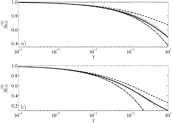
Figure 6: Second and third order correlation functions versus the correlation parameter γ𝛾\gamma. In subplot a) we compare the exact results from Lieb-Liniger theory, gLL(2)subscriptsuperscript𝑔2𝐿𝐿g^{(2)}_{LL} (solid line), and the approximation in the GP-regime, gLL,GP(2)subscriptsuperscript𝑔2𝐿𝐿𝐺𝑃g^{(2)}_{LL,GP} (dashed dotted line) to gx,x(2)g0,0(2)subscriptsuperscript𝑔2𝑥𝑥subscriptsuperscript𝑔200g^{(2)}_{x,x}\equiv g^{(2)}_{0,0} calculated with an extended mean-field theory. We depict exact results (dashed line) using (45) and (46) as well as approximated results (dotted line) using (47). In subplot b) we depict the same comparison for the third order correlation function.

In figure 6 we see a comparison of approximations and exact numerical results within extended mean-field theory as well as Lieb-Liniger theory. In either case we observe a good agreement between our results and Lieb-Liniger theory. However as γ𝛾\gamma increases the deviation from the exact result grows. We attribute this deviation to the non-Gaussian contributions that have been dropped.

Another relevant quantity is the ground state energy of the system. By comparing the value of the energy functional (33) with the Lieb-Liniger ground state energy for a range of the correlation parameter γ𝛾\gamma, we obtain figure 7. In particular, we plot the relative deviation of the ground state energies. This is to be compared with deviations from a simple mean-field approach neglecting fluctuations and for the Bogoliubov method in the GP-regime which includes excitations of the mean-field. The latter approach results in Wadati02

e(γ)LL,GP𝑒subscript𝛾𝐿𝐿𝐺𝑃\displaystyle e(\gamma)_{{LL,GP}} =\displaystyle= γ43πγ32.𝛾43𝜋superscript𝛾32\displaystyle\gamma-\frac{4}{3\pi}\gamma^{\frac{3}{2}}. (60)
Refer to caption
Figure 7: Relative deviations from the dimensionless ground state energy of Lieb-Liniger theory as a function of γ𝛾\gamma. Results from an extended mean-field approach (solid line), the simple mean-field theory without fluctuations (dotted line) and the Bogoliubov approach (dashed dotted line) are compared.

In either case, we present all the results in the form of a normalized deviation from the dimensionless ground state energy e(γ)𝑒𝛾e(\gamma) from Lieb-Liniger theory given by (6).

The results show a clear improvement over simple mean-field theory and it also improves on the Bogoliubov method. Up to the cross-over at γ1𝛾1\gamma\approx 1 the maximum deviation of our results is less than 4%percent\% and we obtain reliable results throughout the region of interest, i.e. γ1𝛾1\gamma\leq 1. However, this appears to be the limit for a quasi one-dimensional extended mean-field theory and different approaches have to be used in the strongly correlated regime.

V Numerical results for trapped atoms at zero and finite temperature

V.1 The zero temperature limit for a trapped gas

In the previous section we have studied the homogeneous case. In here, this will be extended to harmonically trapped systems and we present correlation functions up to third order. First of all we depict the spatial shape of the master variables f~~𝑓\tilde{f}, m~~𝑚\tilde{m} and of the quantities f(c)superscript𝑓𝑐f^{(c)}, m(c)superscript𝑚𝑐m^{(c)}, which are essential for the calculation of the correlation functions. The plots show numerical simulations for a particle number of N=102𝑁superscript102N=10^{2} in a trap with standard parameters for 87Rb according to (34).
Refer to caption
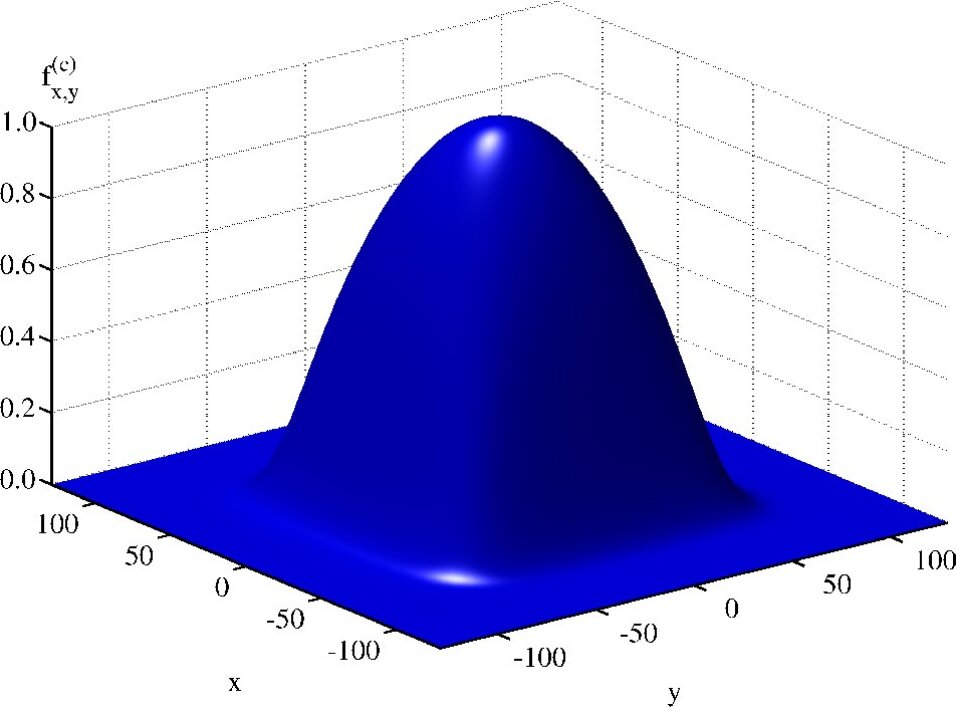
Figure 8: Coherent single particle density matrix fx,y(c)subscriptsuperscript𝑓𝑐𝑥𝑦f^{(c)}_{x,y} versus x𝑥x and y𝑦y. As the ground state is real valued, the coherent part of the pairing field mx,y(c)subscriptsuperscript𝑚𝑐𝑥𝑦m^{(c)}_{x,y} is also represented in this figure.

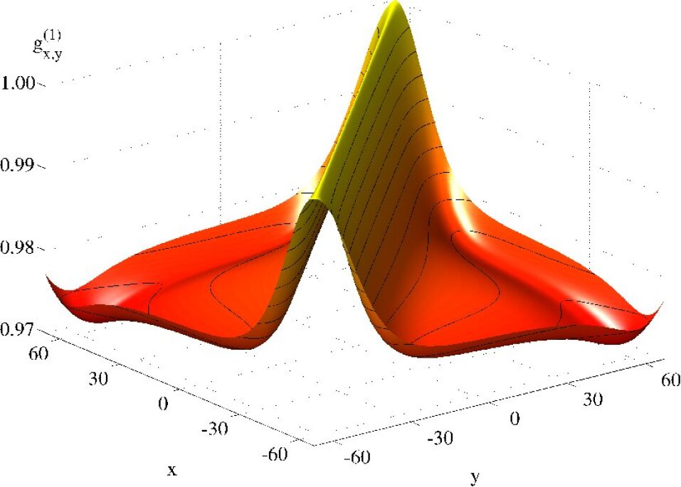
The coherent contribution to the single particle density matrix fx,y(c)subscriptsuperscript𝑓𝑐𝑥𝑦f^{(c)}_{x,y} in figure 8 has off-diagonal long range order and extends over the complete system. As the Hamiltonian for a one-dimensional trap is real-valued, so is the ground state solution αxsubscript𝛼𝑥\alpha_{x}. Hence, the coherent contribution of the pairing field mx,y(c)subscriptsuperscript𝑚𝑐𝑥𝑦m^{(c)}_{x,y} is identical to fx,y(c)subscriptsuperscript𝑓𝑐𝑥𝑦f^{(c)}_{x,y} and shown in figure 8.

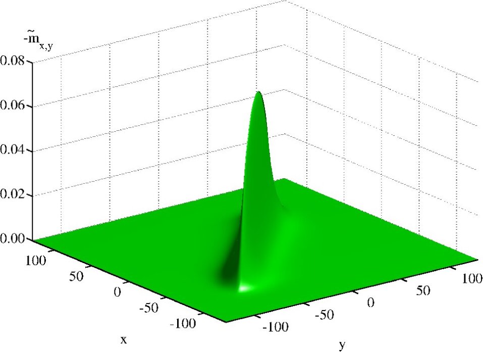
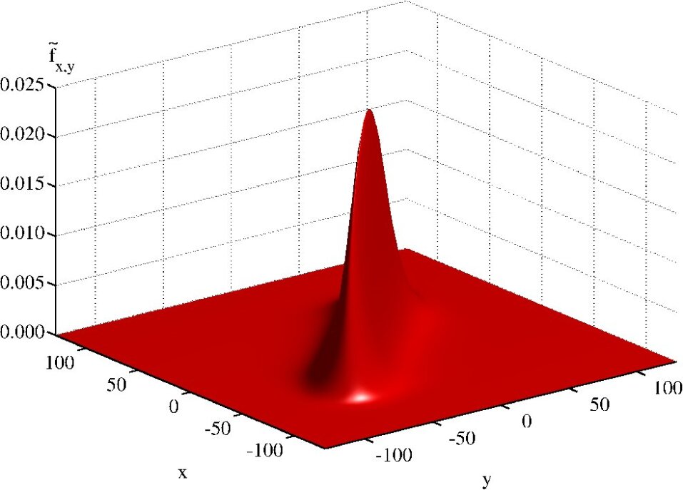
In contrast to the coherent contributions, the normal fluctuation f~x,ysubscript~𝑓𝑥𝑦\tilde{f}_{x,y} in figure 9 and the anomalous fluctuation m~x,ysubscript~𝑚𝑥𝑦\tilde{m}_{x,y} in figure 10 are primarily localized along the diagonal.
Refer to caption
Figure 9: Normal fluctuations f~x,ysubscript~𝑓𝑥𝑦\tilde{f}_{x,y} versus x𝑥x and y𝑦y.
Refer to caption
Figure 10: Anomalous fluctuations m~x,ysubscript~𝑚𝑥𝑦-\tilde{m}_{x,y} versus x𝑥x and y𝑦y.

The coherence in the off-diagonal direction is only of short range and the negativity of the pairing field is an indication of a reduced likelihood of finding two particles at the same location.
Refer to caption
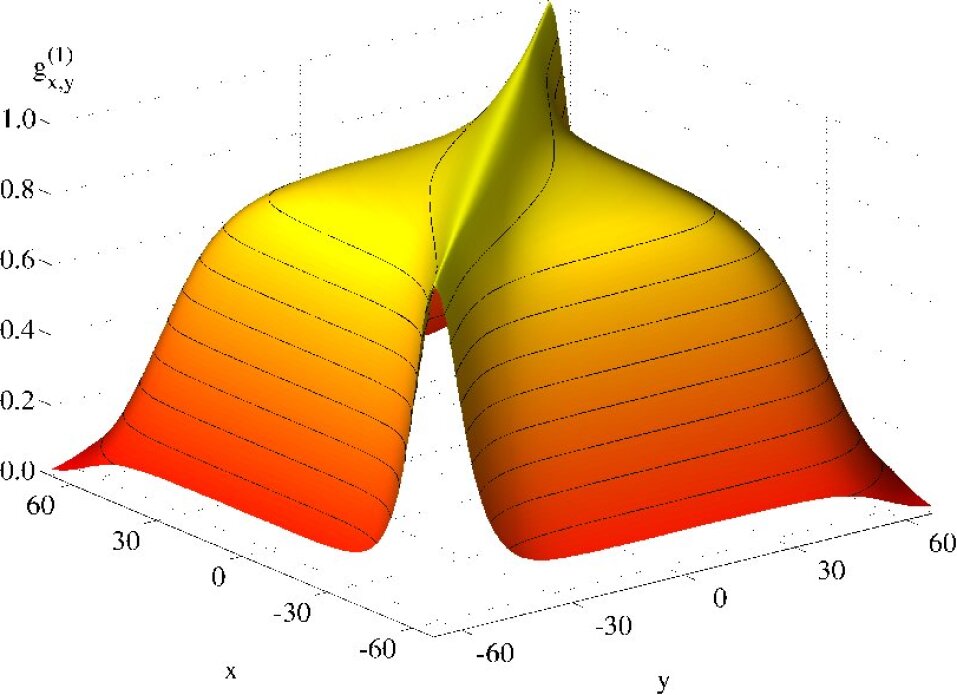
Figure 11: First order correlation function gx,y(1)subscriptsuperscript𝑔1𝑥𝑦g^{(1)}_{x,y} versus x𝑥x and y𝑦y.
Refer to caption
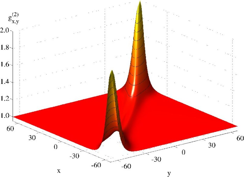
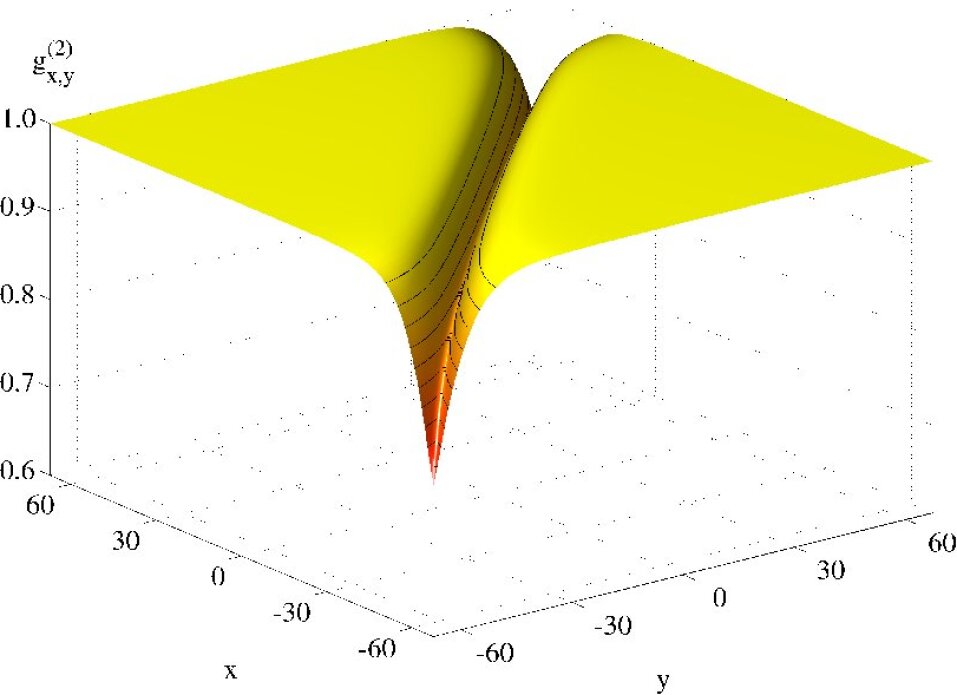
Figure 12: Second order correlation function gx,y(2)subscriptsuperscript𝑔2𝑥𝑦g^{(2)}_{x,y} versus x𝑥x and y𝑦y.
Refer to caption
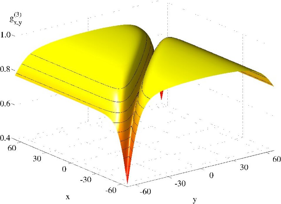
Figure 13: Third order correlation function gx,y(3)subscriptsuperscript𝑔3𝑥𝑦g^{(3)}_{x,y} versus x𝑥x and y𝑦y.

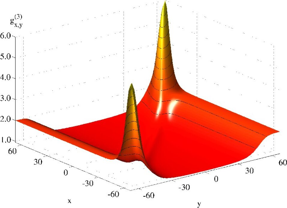
The behaviour of the first, second and third order correlation function is presented in figures 11, 12 and 13. A generic feature of all three correlation functions is that they become more pronounced for smaller particle numbers. For the first order correlation function the diagonal has to be identical to one and the deviation in the off-diagonal is fairly small as expected for a coherent system. However, the second order density-density correlation is a more sensitive probe as this correlation function is less than one, thus exhibits non-classical behaviour. This anti-bunching is particularly strong for smaller particle numbers when we approach the Tonks-Girardeau regime of a fermionized Bose gas and the correlation function vanishes eventually. Recently this effect has been investigated in a number of experiments, e.g. Weiss05 ; Raizen2005 ; Paredes2004 and confirms the theoretical predictions. The same statements apply to the third order correlation function and it can be observed that the deviation from one is even more pronounced. This also implies that the third order correlation function Tolra04 ; cornell597 is the most sensitive probe for quantum aspects of the field. In addition we notice values which are clearly below one for |y|1much-greater-than𝑦1|y|\gg 1 and xy𝑥𝑦x\neq y, because in this case gx,y(3)gy,y(2)subscriptsuperscript𝑔3𝑥𝑦subscriptsuperscript𝑔2𝑦𝑦g^{(3)}_{x,y}\approx g^{(2)}_{y,y}. This can easily be seen by looking at (58,IV.3) and taking into account that all terms with off-diagonal contributions of the fluctuations in gx,y(3)subscriptsuperscript𝑔3𝑥𝑦g^{(3)}_{x,y} are negligible for xy𝑥𝑦x\neq y.

V.2 Behaviour in the center of the trap
Refer to caption
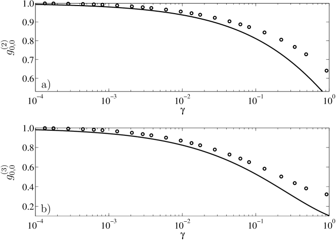
Figure 14: Correlation functions versus the correlation parameter γ𝛾\gamma. In subplot a) we depict g0,0(2)subscriptsuperscript𝑔200g^{(2)}_{0,0} and compare simulation results for the trapped case (circles) with analytic calculations obtained with Lieb-Liniger theory (solid line). In subplot b) we depict g0,0(3)subscriptsuperscript𝑔300g^{(3)}_{0,0} and again compare simulation results for the trapped case (circles) with analytic calculations obtained with Lieb-Liniger theory (solid line). In both comparisons the circles originate for particle numbers N𝑁N ranging from N=105𝑁superscript105N=10^{5} on the left hand side to N=100𝑁superscript100N=10^{0} on the right hand side.

In figure 14 we compare the results of our simulations for the second and third order correlation function with Lieb-Liniger theory. In contrast to the comparison in subsection IV.3 an external potential is now included in the calculations with the extended mean-field theory whereas the theoretical curve is for a homogeneous gas of bosons. Our simulations are for particle numbers ranging from N=100105𝑁superscript100superscript105N=10^{0}-10^{5} and we only used the values of the correlation functions in the center of the trap for the comparison. Compared to subsection IV.3 the results in the trapped case deviate slightly more from the exact results originating from the homogeneous Lieb-Liniger theory but the qualitative behaviour is very similar.

V.3 Diagonal behaviour in the local density approximation

The local density approximation (LDA) is a frequently employed approximation scheme to transfer results of homogeneous systems to spatially trapped gases. It is assumed that a smooth variation of the density profile can be incorporated by an adiabatic adjustment of a locally uniform gas. The LDA uses a local effective chemical potential Shlyap05

μ(x)=μ0V(x)=μ012mω2x2,𝜇𝑥subscript𝜇0𝑉𝑥subscript𝜇012𝑚superscript𝜔2superscript𝑥2\displaystyle\mu(x)=\mu_{0}-V(x)=\mu_{0}-\frac{1}{2}m\omega^{2}x^{2}\;, (61)

where μ0subscript𝜇0\mu_{0} denotes the global equilibrium chemical potential. In order for the LDA to be applicable, it is thus necessary that the short-range correlation length is much smaller than the characteristic inhomogeneity length.
Refer to caption
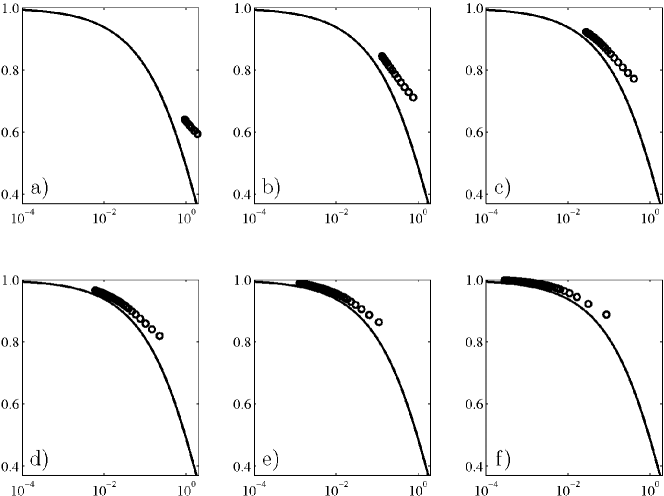
Figure 15: The diagonal second order correlation function gx,x(2)subscriptsuperscript𝑔2𝑥𝑥g^{(2)}_{x,x} versus γ𝛾\gamma for various particle numbers. With an increasing value of the correlation parameter γ𝛾\gamma the circles correspond to points further outwards from the origin. We compare results for the trapped case (circles) with analytic calculations for the second order correlation function obtained with LDA-Lieb-Liniger theory (solid line). Plots a) to c) are for N=100𝑁superscript100N=10^{0} , N=101𝑁superscript101N=10^{1} and N=102𝑁superscript102N=10^{2} (from left to right) and plots d) to f) are for N=103𝑁superscript103N=10^{3}, N=104𝑁superscript104N=10^{4} and N=105𝑁superscript105N=10^{5} (from left to right).

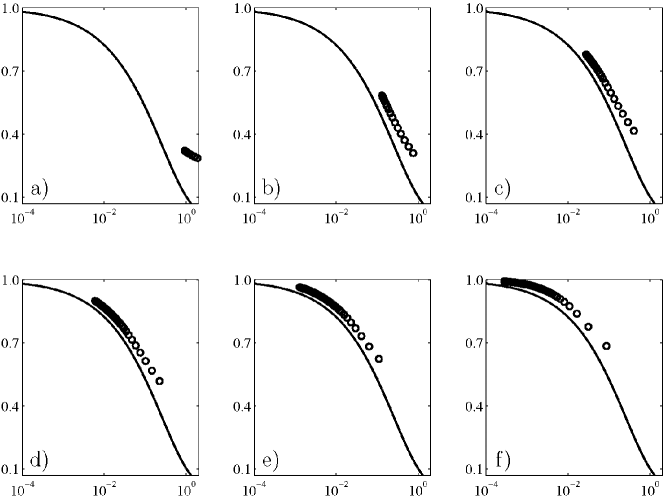
In this context, we want to compare the diagonal behaviour of our numerically calculated correlation functions to theoretical predictions. By definition, the first order correlation function is identical to one along the diagonal and our data behaves accordingly. For the second and third order correlation function we will compare our results with the predictions from Lieb-Liniger theory in the LDA. Naturally the LDA works best in the center of the trap. It can not be expected to work in regions where the density drops rapidly and the inhomogeneity length is very small in these regions.
Refer to caption
Figure 16: The diagonal third order correlation function gx,x(3)subscriptsuperscript𝑔3𝑥𝑥g^{(3)}_{x,x} versus γ𝛾\gamma for various particle numbers. With an increasing value of the correlation parameter γ𝛾\gamma the circles correspond to points further outwards from the origin. We compare results for the trapped case (circles) with analytic calculations for the third order correlation function obtained with LDA-Lieb-Liniger theory (solid line). Plots a) to c) are for N=100𝑁superscript100N=10^{0} , N=101𝑁superscript101N=10^{1} and N=102𝑁superscript102N=10^{2} (from left to right) and plots d) to f) are for N=103𝑁superscript103N=10^{3}, N=104𝑁superscript104N=10^{4} and N=105𝑁superscript105N=10^{5} (from left to right).

In the Gross-Pitaevskii regime the chemical potential μ𝜇\mu connects the density n𝑛n to the correlation parameter γ𝛾\gamma, via

μ(x)=gn(x),γ(x)=mg2n(x).formulae-sequence𝜇𝑥𝑔𝑛𝑥𝛾𝑥𝑚𝑔superscriptPlanck-constant-over-2-pi2𝑛𝑥\displaystyle\mu(x)=gn(x),\quad\gamma(x)=\frac{mg}{\hbar^{2}n(x)}. (62)

In our simulations we tune the particle number in the trap, which decreases γ𝛾\gamma for an increasing number of particles. Qualitatively one can expect that the inhomogeneous correlation functions are higher than the homogeneous results because in the LDA the external potential leads to a smaller chemical potential and according to (62) also to a smaller density compared to the homogeneous case. Due to the monotonous decrease of the correlation functions, there is a tendency of the inhomogeneous values to be shifted to larger γ𝛾\gamma values. All the features that have just been described can be seen in figures 15 and 16, where we plotted the correlation functions for particle numbers ranging from N=100105𝑁superscript100superscript105N=10^{0}-10^{5} and restricted the plotted regions to the Thomas-Fermi radius.

V.4 The finite temperature result for a trapped gas

The zero-temperature results of the previous section can be extended easily to account for finite temperature effects walser04 ; Blaizot_ . One obtains an equilibrium solution for the density matrix G𝐺G of the thermal system (21) from the eigenstates of the selfenergy matrix (29), according to the Bose-Einstein distribution. We present results in the present section for a particle number of N=100𝑁100N=100 and a temperature T=10ω/kB𝑇10Planck-constant-over-2-pi𝜔subscript𝑘𝐵T=10\;\hbar\omega/k_{B}.

Refer to caption
Figure 17: Finite temperature first order correlation function gx,y(1)subscriptsuperscript𝑔1𝑥𝑦g^{(1)}_{x,y} versus x𝑥x and y𝑦y, for N=100𝑁100N=100 and T=10ω/kB𝑇10Planck-constant-over-2-pi𝜔subscript𝑘𝐵T=10\;\hbar\omega/k_{B}.
Refer to caption
Figure 18: Finite temperature second order correlation function gx,y(2)subscriptsuperscript𝑔2𝑥𝑦g^{(2)}_{x,y} versus x𝑥x and y𝑦y, for N=100𝑁100N=100 and T=10ω/kB𝑇10Planck-constant-over-2-pi𝜔subscript𝑘𝐵T=10\;\hbar\omega/k_{B}.
Refer to caption
Figure 19: Finite temperature third order correlation function gx,y(3)subscriptsuperscript𝑔3𝑥𝑦g^{(3)}_{x,y} versus x𝑥x and y𝑦y, for N=100𝑁100N=100 and T=10ω/kB𝑇10Planck-constant-over-2-pi𝜔subscript𝑘𝐵T=10\;\hbar\omega/k_{B}.

The main thermal effect is a strong increase of the fluctuations at the edge of the trap at the cost of a reduction of the condensate density Hutchinson97 . This effect is clearly seen by comparing the first order correlation function in figure 17 to the zero temperature result in figure 11. At finite temperatures, we also obtain a reduction of first order coherence. Consequently, this leads to a situation where the gas is almost thermalized at the edge of the trap, whereas it is coherent in the center. The suppression of density fluctuations, also known as anti-bunching, is also less pronounced at finite temperature. This can be seen by comparing figures 18 and 19 to figures 12 and 13, which give the zero temperature results.

For a thermal gas of noninteracting bosons, one finds g0,0(2)=2!subscriptsuperscript𝑔2002g^{(2)}_{0,0}=2! and g0,0(3)=3!subscriptsuperscript𝑔3003g^{(3)}_{0,0}=3!. It can be seen that these values are attained at the edge of the trap where fluctuations dominate. In figure 19 we also notice a value of two for |y|1much-greater-than𝑦1|y|\gg 1 and xy𝑥𝑦x\neq y, because we again have gx,y(3)gy,y(2)=2subscriptsuperscript𝑔3𝑥𝑦subscriptsuperscript𝑔2𝑦𝑦2g^{(3)}_{x,y}\approx g^{(2)}_{y,y}=2 in this case.

Refer to caption
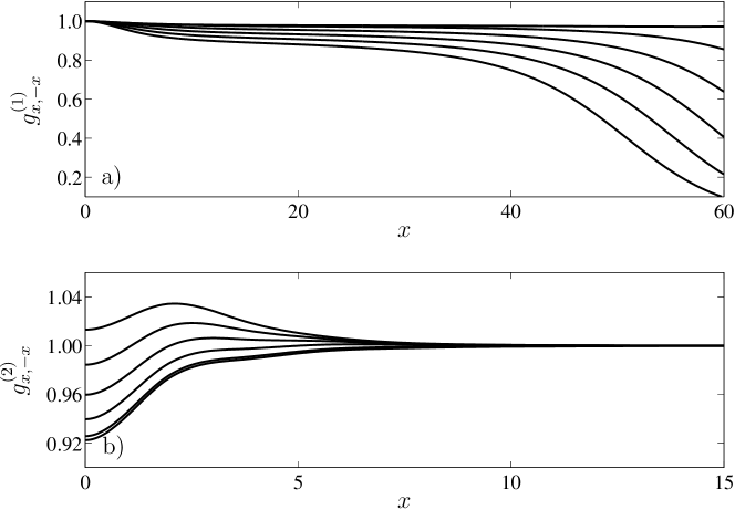
Figure 20: Off-diagonal first gx,x(1)subscriptsuperscript𝑔1𝑥𝑥g^{(1)}_{x,-x} (a) and second order correlation function gx,x(2)subscriptsuperscript𝑔2𝑥𝑥g^{(2)}_{x,-x} (b) versus x𝑥x. The individual curves correspond to temperatures kBT=0ωsubscript𝑘𝐵𝑇0Planck-constant-over-2-pi𝜔k_{B}T=0\,\hbar\omega (smallest value for x=0𝑥0x=0) to 10ω10Planck-constant-over-2-pi𝜔10\,\hbar\omega (largest value for x=0𝑥0x=0) with increments of 2ω2Planck-constant-over-2-pi𝜔2\,\hbar\omega.

In figure 20, we present the off-diagonal of the first and second-order correlation function gx,x(1,2)subscriptsuperscript𝑔12𝑥𝑥g^{(1,2)}_{x,-x} versus x𝑥x for temperatures from kBT=010ωsubscript𝑘𝐵𝑇010Planck-constant-over-2-pi𝜔k_{B}T=0-10\,\hbar\omega with increments of 2ω2Planck-constant-over-2-pi𝜔2\,\hbar\omega. It can be noticed that correlations are strongly attenuated with increasing temperature. Looking at the off-diagonal of gx,x(2)subscriptsuperscript𝑔2𝑥𝑥g^{(2)}_{x,-x} in figure 20, we see a reduction of the anti-bunching dip in the center with increasing temperatures, however it is still present for high values of the temperature. It can be understood qualitatively from the stronger increase of fluctuations with the temperature at the edge of the trap. Thus, the anti-bunching dip in the center of the trap remains visible even at finite temperatures.

VI Conclusions and outlook

We have presented a detailed study of an extended mean-field theory which shows that it is a feasible approach for the description of a weakly correlated gas of bosons in a quasi-1D setup. This approach agrees well with exact predictions of zero-temperature Lieb-Liniger theory and can easily be applied to spatially inhomogeneous systems at finite temperature. We have not analyzed the finite temperature theory of Yang-Yang due its complexity.

There are many relevant applications for using this extended mean-field theory in different geometrical configurations like a double-well potential Oberthaler05 ; Oberthaler06a . Yet another extension of our approach is the dimensional crossover out-of-equilibrium where in general the increase of available phase space volume leads to a decrease of correlations. An evaluation of the such correlation functions is work in progress.

Acknowledgments

The authors acknowledge the support by the German Research Foundation via SFB/TRR 21 which is a collaboration of the Universities of Stuttgart, Tübingen, Ulm and the Max Planck Institute for Solid State Research in Stuttgart.

Appendix A Higher transcendental functions

A.1 Complete elliptic integrals

Following the definitions and the notation in Abramowitz , the complete elliptic integral of the first kind reads

K(m)𝐾𝑚\displaystyle K(m) =\displaystyle= 0π/2dθ1msin2θ,superscriptsubscript0𝜋2d𝜃1𝑚superscript2𝜃\displaystyle\int_{0}^{\pi/2}\frac{{\rm d}\theta}{\sqrt{1-m\sin^{2}\theta}}, (63)

where the parameter 0m10𝑚10\leq m\leq 1. For the calculation of m~0subscript~𝑚0\tilde{m}_{0} in section IV.1, we encounter an integral of the form

I1=0dkk2+ωck2+ω~=K(m)kcsubscript𝐼1superscriptsubscript0d𝑘superscript𝑘2subscript𝜔𝑐superscript𝑘2~𝜔𝐾𝑚subscript𝑘𝑐\displaystyle I_{1}=\int_{0}^{\infty}\frac{{\rm d}k}{\sqrt{k^{2}+\omega_{c}}\sqrt{k^{2}+{\tilde{\omega}}}}=\frac{K(m)}{k_{c}} (64)

where ωc>ω~subscript𝜔𝑐~𝜔\omega_{c}>{\tilde{\omega}}. We can show that the evaluation of this integral leads to the complete elliptic integral of the first kind by making the substitution k=kccotθ𝑘subscript𝑘𝑐𝜃k=k_{c}\cot\theta and using m=(ωcω~)/ωc𝑚subscript𝜔𝑐~𝜔subscript𝜔𝑐m=(\omega_{c}-{\tilde{\omega}})/\omega_{c}.

Similarly the complete elliptic integral of the second kind is defined as

E(m)𝐸𝑚\displaystyle E(m) =\displaystyle= 0π/21msin2θdθ.superscriptsubscript0𝜋21𝑚superscript2𝜃differential-d𝜃\displaystyle\int_{0}^{\pi/2}{\sqrt{1-m\sin^{2}\theta}}\,{\rm d}\theta\;. (65)

In order to calculate f~0subscript~𝑓0\tilde{f}_{0} in section IV.1 we end up with the integral

I2=0dkk2+ωck2+ω~k2+ω~subscript𝐼2superscriptsubscript0differential-d𝑘superscript𝑘2subscript𝜔𝑐superscript𝑘2~𝜔superscript𝑘2~𝜔\displaystyle I_{2}=\int_{0}^{\infty}{\rm d}k\,\frac{\sqrt{k^{2}+\omega_{c}}-\sqrt{k^{2}+{\tilde{\omega}}}}{\sqrt{k^{2}+{\tilde{\omega}}}} (66)

after separating the constant contribution which leads to the previously discussed integral. The same substitution as above k=kccotθ𝑘subscript𝑘𝑐𝜃k=k_{c}\cot\theta simplifies the integral to the form

I2=kc0π/211msin2θsin2θ1msin2θdθ=kc(E(m)K(m)).subscript𝐼2subscript𝑘𝑐superscriptsubscript0𝜋211𝑚superscript2𝜃superscript2𝜃1𝑚superscript2𝜃differential-d𝜃subscript𝑘𝑐𝐸𝑚𝐾𝑚\displaystyle I_{2}=k_{c}\int_{0}^{\pi/2}\frac{1-\sqrt{1-m\sin^{2}\theta}}{\sin^{2}\theta\sqrt{1-m\sin^{2}\theta}}\,{\rm d}\theta=-k_{c}\left(E(m)-K(m)\right)\;. (67)

A.2 The Lambert-W function

The Lambert-W𝑊W-function is implicitly defined by the solution of the transcendental equation knuth96

z=WeW.𝑧𝑊superscript𝑒𝑊z=We^{W}. (68)

In the case of large arguments z1much-greater-than𝑧1z\gg 1, one can use an asymptotic expansion

W(z)=12+2/1+,𝑊𝑧subscript1subscript2subscript2subscript1W(z)=\ell_{1}-\ell_{2}+\ell_{2}/\ell_{1}+\ldots, (69)

with 1=lnzsubscript1𝑧\ell_{1}=\ln z and 2=lnlnzsubscript2𝑧\ell_{2}=\ln\ln z.

Appendix B Deformation of the integration contour in the complex plane

The results of subsection IV.2.2 can be derived alternatively with the help of complex integration Migdal . If we take the inverse Fourier transform of the anomalous fluctuation of (42), we get

m~(r)=ω4πeikrk2+ωck2+ω~𝑑k.~𝑚𝑟subscript𝜔4𝜋superscriptsubscriptsuperscript𝑒𝑖𝑘𝑟superscript𝑘2subscript𝜔𝑐superscript𝑘2~𝜔differential-d𝑘\displaystyle{\tilde{m}}\left({r}\right)=-\frac{\omega_{-}}{4\pi}\int_{-\infty}^{\infty}\frac{e^{-ikr}}{\sqrt{k^{2}+\omega_{c}}\sqrt{k^{2}+{\tilde{\omega}}}}\,dk\;. (70)

Using the substitutions k=k~z𝑘~𝑘𝑧k={\tilde{k}}z, r=k~rsuperscript𝑟~𝑘𝑟r^{\prime}={\tilde{k}}r and b2=kc2/k~2superscript𝑏2superscriptsubscript𝑘𝑐2superscript~𝑘2b^{2}=k_{c}^{2}/{\tilde{k}}^{2} this equation reduces to

m~(r)=ω4πeirzz2+b2z2+1dzk~.~𝑚𝑟subscript𝜔4𝜋superscriptsubscriptsuperscript𝑒𝑖superscript𝑟𝑧superscript𝑧2superscript𝑏2superscript𝑧21𝑑𝑧~𝑘\displaystyle{\tilde{m}}\left({r}\right)=-\frac{\omega_{-}}{4\pi}\int_{-\infty}^{\infty}\frac{e^{-ir^{\prime}z}}{\sqrt{z^{2}+b^{2}}\sqrt{z^{2}+1}}\,\frac{dz}{{\tilde{k}}}\;. (71)

For the evaluation of this integral we make a branch cut between i𝑖-i and ib𝑖𝑏-ib and choose the path of integration as can be seen in Fig. 21.

Refer to caption
Figure 21: Integration contour for the evaluation of (70).

The contributions from C1subscript𝐶1C_{1} and C6subscript𝐶6C_{6} vanish if the contour is moved to infinity and the contributions from C2subscript𝐶2C_{2} and C5subscript𝐶5C_{5} cancel each other. The integrals along the semicircles around ib𝑖𝑏-ib and the circle around i𝑖-i tend to zero if the radius tends to zero. Due to the branch cut the contributions from C3subscript𝐶3C_{3} and C4subscript𝐶4C_{4} are equal. Thus, the integral to be solved reads

I𝐼\displaystyle I =\displaystyle\!=\! eirzdzz2+1z2+b2=ibi2eirzdzz2+1z2+b2superscriptsubscriptsuperscript𝑒𝑖superscript𝑟𝑧𝑑𝑧superscript𝑧21superscript𝑧2superscript𝑏2superscriptsubscript𝑖𝑏𝑖2superscript𝑒𝑖superscript𝑟𝑧𝑑𝑧superscript𝑧21superscript𝑧2superscript𝑏2\displaystyle\!\int_{-\infty}^{\infty}\!\frac{e^{-ir^{\prime}z}dz}{\sqrt{z^{2}+1}\sqrt{z^{2}+b^{2}}}=\int_{-ib}^{-i}\!\frac{2e^{-ir^{\prime}z}dz}{\sqrt{z^{2}+1}\sqrt{z^{2}+b^{2}}} (72)

and by changing the variable of integration (z=iiy𝑧𝑖𝑖𝑦z=-i-iy), taking into account that b1much-greater-than𝑏1b\gg 1 in the Gross-Pitaevskii regime, we get

I𝐼\displaystyle I \displaystyle\approx 2er0eyrdy2y+y2b212yy2.2superscript𝑒superscript𝑟superscriptsubscript0superscript𝑒𝑦superscript𝑟𝑑𝑦2𝑦superscript𝑦2superscript𝑏212𝑦superscript𝑦2\displaystyle 2e^{-r^{\prime}}\int_{0}^{\infty}\frac{e^{-yr^{\prime}}dy}{\sqrt{2y+y^{2}}\sqrt{b^{2}-1-2y-y^{2}}}\;. (73)

As we are looking for an approximation for r=k~r1superscript𝑟~𝑘𝑟much-greater-than1r^{\prime}={\tilde{k}}r\gg 1, we notice that only small values of y𝑦y play an important role for the evaluation of the integral.

Hence we neglect the expression 1+2y+y212𝑦superscript𝑦21+2y+y^{2} in the second term in the denominator which yields

I𝐼\displaystyle I \displaystyle\approx 2erb20eyr2y+y2𝑑y=2b2K0(r)2superscript𝑒superscript𝑟superscript𝑏2superscriptsubscript0superscript𝑒𝑦superscript𝑟2𝑦superscript𝑦2differential-d𝑦2superscript𝑏2subscript𝐾0superscript𝑟\displaystyle 2\frac{e^{-r^{\prime}}}{\sqrt{b^{2}}}\int_{0}^{\infty}\frac{e^{-yr^{\prime}}}{\sqrt{2y+y^{2}}}\,dy\;=\;\frac{2}{\sqrt{b^{2}}}\,K_{0}(r^{\prime}) (74)

and as m~~𝑚\tilde{m} is an even function in r𝑟r we get the final result

m~(r)~𝑚𝑟\displaystyle\tilde{m}(r) \displaystyle\approx ω2πkcK0(k~|r|)kc4πK0(k~|r|).subscript𝜔2𝜋subscript𝑘𝑐subscript𝐾0~𝑘𝑟subscript𝑘𝑐4𝜋subscript𝐾0~𝑘𝑟\displaystyle-\frac{\omega_{-}}{2\pi k_{c}}K_{0}({\tilde{k}}|r|)\;\approx\;-\frac{k_{c}}{4\pi}\;K_{0}({\tilde{k}}|r|)\;. (75)

References

  • (1) A. Görlitz et al., Phys. Rev. Lett. 87, 130402 (2001).
  • (2) H. Moritz, T. Stoferle, M. Kohl, and T. Esslinger, Phys. Rev. Lett. 91, 250402 (2003).
  • (3) B. Laburthe Tolra et al., Phys. Rev. Lett. 92, 190401 (2004).
  • (4) D. Hellweg et al., Phys. Rev. Lett. 91, 010406 (2003).
  • (5) T. Kinoshita, T. Wenger, and D. S. Weiss, Phys. Rev. Lett. 95, 190406 (2005).
  • (6) C.-S. Chuu et al., Phys. Rev. Lett. 95, 260403 (2005).
  • (7) A.H. van Amerongen et al., Preprint arXiv:0709.1899, (2007).
  • (8) S. Hofferberth et al., Nature 449, 324 (2007).
  • (9) The Many-Body Problem: An Encyclopedia of Exactly Solved Models in One Dimension, edited by D. C. Mattis, World Scientific, Singapore (1995).
  • (10) M. Girardeau, J. Math. Phys. 1, 516 (1960).
  • (11) E. Lieb and W. Lininger, Phys. Rev. 130, 1605 (1963).
  • (12) C. N. Yang and C. P. Yang, J. Math. Phys. 10, 1115 (1969).
  • (13) K. K. Das, M. D. Girardeau, and E. M. Wright, Phys. Rev. Lett. 89, 110402 (2002).
  • (14) B. Paredes et al., Nature 429, 277 (2004).
  • (15) B. D. Esry, Phys. Rev. A 55, 1147 (1997).
  • (16) O. E. Alon, A. I. Streltsov, K. Sakmann, and L. S. Cederbaum, Europhysics Letters 67, 8 (2004).
  • (17) S. Zöllner, H.-D. Meyer, and P. Schmelcher, Phys. Rev. A 74, 063611 (2006).
  • (18) A. I. Streltsov, O. E. Alon, and L. S. Cederbaum, Phys. Rev. A 73, 063626 (2006).
  • (19) S. R. White, Phys. Rev. Lett. 69, 2863 (1992).
  • (20) D. Jaksch et al., Phys. Rev. Lett. 81, 3108 (1998).
  • (21) D. van Oosten, P. van der Straten, and H. T. C. Stoof, Phys. Rev. A 63, 053601 (2001).
  • (22) M. Rigol and A. Muramatsu, Phys. Rev. Lett. 94, 240403 (2005).
  • (23) C. Kollath, U. Schollwöck, J. von Delft, and W. Zwerger, Phys. Rev. A 69, 031601 (2004).
  • (24) M. Aizenman et al., Phys. Rev. A 70, 023612 (2004).
  • (25) P. D. Drummond and P. Deuar, J. Opt. B: Quantum Semiclass. Opt. 5, S281 (2003).
  • (26) M. Yasuda and F. Shimizu, Phys. Rev. Lett. 77, 3090 (1996).
  • (27) P. Bouyer and M. Kasevich, prepint (1996).
  • (28) B. Saubaméa et al., Phys. Rev. Lett. 79, 3146 (1997).
  • (29) A. Perrin et al., Phys. Rev. Lett. 99, 150405 (2007).
  • (30) E. A. Burt et al., Phys. Rev. Lett. 79, 337 (1997).
  • (31) Y. Kagan, B. V. Svistunov, and G. V. Shlyapnikov, JETP Lett. 42, 209 (1985).
  • (32) D. S. Petrov, G. V. Shlyapnikov, and J. T. M. Walraven, Phys. Rev. Lett. 85, 3745 (2000).
  • (33) M. Olshanii and V. Dunjko, Phys. Rev. Lett. 91, 090401 (2003).
  • (34) D. M. Gangardt and G. V. Shlyapnikov, New J. Phys. 5, 79.1 (2003).
  • (35) D. M. Gangardt and G. V. Shlyapnikov, Phys. Rev. Lett. 90, 010401 (2003).
  • (36) R. Walser, Opt. Comm. 243, 107 (2004).
  • (37) N. M. Bogoliubov, C. Malyshev, R. K. Bullough, and J. Timonen, Phys. Rev. A 69, 023619 (2004).
  • (38) K. V. Kheruntsyan, D. M. Gangardt, P. D. Drummond, and G. V. Shlyapnikov, Phys. Rev. A 71, 053615 (2005).
  • (39) G. E. Astrakharchik and S. Giorgini, J. Phys. B 39, S1 (2006).
  • (40) V. V. Cheianov, H. Smith, and M. B. Zvonarev, Phys. Rev. A 73, 051604 (2006).
  • (41) V. V. Cheianov, H. Smith, and M. B. Zvonarev, cond-mat 0602468 (2006).
  • (42) R. Walser, J. Williams, J. Cooper, and M. Holland, Phys. Rev. A 59, 3878 (1999).
  • (43) M. Holland, J. Park, and R. Walser, Phys. Rev. Lett. 86, 1915 (2001).
  • (44) M. Holland, S. Kokkelmans, M. Chiofalo, and R. Walser, Phys. Rev. Lett. 87, 120406 (2001).
  • (45) R. P. Feynman, Phys. Rev. 56, 340 (1939).
  • (46) A. I. Akhiezer and S. V. Peletminskii, Methods of Statistical Physics, Pergamon Press Ltd., Oxford, England (1981).
  • (47) D. Zubarev, V. Morozov, and G. Röpke, Statistical Mechanics of Nonequilibrium Processes, Akademie Verlag, Berlin (1997).
  • (48) S. Chapman and T. G. Cowling, The Mathematical Theory of Non-Uniform Gases, Cambridge University Press, Cambridge (1970).
  • (49) J.-P. Blaizot and G. Ripka, Quantum Theory of Finite Systems, The MIT Press, Cambridge, Massachusetts (1986).
  • (50) J. Wachter, R. Walser, J. Cooper, and M. Holland, Phys. Rev. A 64, 053612 (2001).
  • (51) M. Olshanii, Phys. Rev. Lett. 81, 938 (1998).
  • (52) C. Menotti and S. Stringari, Phys. Rev. A 66, 043610 (2002).
  • (53) A. Griffin, Phys. Rev. B 53, 9341 (1996).
  • (54) Handbook of Mathematical Functions, edited by M. Abramowitz and I. A. Stegun, Dover Publications, Inc., New York (1972).
  • (55) R. Corless et al., Adv. Comp. Maths. 5, 329 (1996).
  • (56) M. Wadati, J. Phys. Soc. Jpn. 71, 2657 (2002).
  • (57) D. A. W. Hutchinson, E. Zaremba, and A. Griffin, Phys. Rev. Lett. 78, 1842 (1997).
  • (58) M. Albiez et al., Phys. Rev. Lett. 95, 010402 (2005).
  • (59) R. Gati et al., Phys. Rev. Lett. 96, 130404 (2006).
  • (60) A. B. Migdal, Qualitative Methods in Quantum Theory, W.A. Benjamin, Inc., Reading, Massachusetts (1977).