Tidal Disruption of Stellar Objects by Hard Supermassive Black Hole Binaries

Abstract

Supermassive black hole binaries (SMBHBs) are expected by the hierarchical galaxy formation model in $\Lambda$CDM cosmology. There is some evidence in the literature for SMBHBs in AGNs, but there are few observational constraints on the evolution of SMBHBs in inactive galaxies and gas-poor mergers. On the theoretical front, it is unclear how long is needed for a SMBHB in a typical galaxy to coalesce. In this paper we investigate the tidal interaction between stars and binary BHs and calculate the tidal disruption rates of stellar objects by the BH components of binary. We derive the interaction cross sections between SMBHBs and stars from intensive numerical scattering experiments with particle number $\sim 10^{7}$ and calculate the tidal disruption rates by both single and binary BHs for a sample of realistic galaxy models, taking into account the general relativistic effect and the loss cone refilling because of two-body interaction. We estimate the frequency of tidal flares for different types of galaxies using the BH mass function in the literature. We find that because of the three-body slingshot effect, the tidal disruption rate in SMBHB system is more than one order of magnitude smaller than that in single SMBH system. The difference is more significant in less massive galaxies and does not depend on detailed stellar dynamical processes. Our calculations suggest that comparisons of the calculated tidal disruption rates for both single and binary BHs and the surveys of X-ray or UV flares at galactic centers could tell us whether most SMBHs in nearby galaxies are single and whether the SMBHBs formed in gas-poor galaxy mergers coalesce rapidly.

1 INTRODUCTION

In cold dark matter (CDM) cosmology, galaxies form hierarchically and present-day galaxies are the products of successive mergers (Kauffmann & Haehnelt, 2000; Springel et al., 2005). Recent observations show that almost all galaxies harbor supermassive black holes (SMBHs) at their centers (Richstone et al., 1998; Ferrarese & Ford, 2005) and the black hole (BH) masses tightly correlate with the properties of their host galaxies such as the mass of stellar bulge (Magorrian et al., 1998; Häring & Rix, 2004), the bulge luminosity (McLure & Dunlop, 2002), and the nuclear stellar velocity dispersion (Ferrarese & Merritt, 2000; Gebhardt et al., 2000; Tremaine et al., 2002). The correlations between BH mass and galaxy properties imply that the growth of SMBHs and the formation and evolution of galaxies are closely linked. The correlation is likely induced by galaxy major mergers (merging of galaxies with comparable mass) in which both rapid star formation and gas accretion onto SMBHs are triggered and the feedback from the central active galactic nuclei (AGNs) regulates the growth of both SMBHs and galaxy bulges. The coevolution scenario can successfully explain not only the correlations between SMBHs and their host galaxies but also many of the observed evolutions of galaxies and AGNs (Springel et al., 2005; Hopkins et al., 2006; Croton et al., 2006).

During galaxy mergers part of the gas originally in galactic plane is driven to galaxy center, triggering starburst and the accretion of central SMBH (Gaskell, 1985; Hernquist & Mihos, 1995). If both galaxies in the merging system harbor SMBHs at their centers, a pair of AGNs could form which is an intriguing object for both observations and theories. Because of dynamical friction the two SMBHs quickly sink to the common center of the two merging galaxies, forming a bound, compact ($\sim 10$ pc) supermassive black hole binary (SMBHB, Begelman et al., 1980), which would be difficult to resolve in any but the closest galaxies using current telescopes. As the separation of the binary shrinks, dynamical friction becomes less and less efficient and three-body interaction between SMBHB and the stars passing by becomes more and more important. At separations $\sim 0.1-1$ pc SMBHB becomes hard in the sense that the binary loses energy and angular momentum mainly through three-body interaction. The stars passing by the binary, if not tidally disrupted or swallowed by the BHs, would be expelled by the “slingshot effect” (Quinlan, 1996, Q96 thereafter) with velocities comparable to the host galaxy’s escape velocity. If the refilling of the reservoir of stars on orbits that interact with the SMBHB is inefficient, the evolution of SMBHB slows down and the evolution timescale may even exceed the Hubble time, with the SMBHB separation stalling well outside the radii needed for the final gravitational wave radiation and coalescence stage (Yu, 2002, Y02 hereafter). This seems inconsistent with that fact that SMBHBs have not yet been observed in nearby galaxies. Therefore, many stellar-dynamical mechanisms are proposed to boost the hardening rate of SMBHBs in gas-poor systems, including non-equilibrium stellar distribution (Milosavljević & Merritt, 2003), Brownian motion of SMBHB (Chatterjee et al., 2003), and non-spherical (axisymmetric, triaxial, or irregular) stellar distribution (Y02; Merritt & Poon, 2004; Berczik et al., 2006). However, the conclusions in the above scenarios depend on processes which are not well understood, so it is still unclear whether SMBHBs could coalesce within a Hubble time using purely stellar-dynamical processes. In gas-rich systems it has been argued that the interaction between binary BHs and the gaseous environment could efficiently drive the binary to the gravitational radiation dominant domain within a timescale of $\sim 10^{7}~{}{\rm yr}$ (Ivanov et al., 1999; Gould & Rix, 2000; Armitage & Natarajan, 2002; Escala et al., 2005; Kazantzidis et al., 2005).

Although many physical processes have been proposed in the literature to boost the hardening rates of SMBHBs, the abundance of binary BHs in galaxy centers has not yet been strongly constrained observationally. Because of their compactness, bound SMBHBs are very difficult to resolve directly with current telescopes, and only unbound SMBHBs in a couple of gas-rich (wet) galaxy mergers have been identified (Komossa, 2006). So far all the evidence for bound and hard SMBHBs are indirect and model dependent. The prototype evidence for SMBHBs in AGNs is the helical morphology of radio jets in many radio galaxies which may be due to the precession of jet orientation in a SMBHB system (Begelman et al., 1980). It has been suggested that the periodic outbursts observed in some AGNs (Sillanpää et al., 1988; Liu et al., 1995, 1997; Raiteri et al., 2001) are due to the orbital motion of the jet-emitting BH in SMBHB (Villata & Raiteri, 1999; Ostorero et al., 2004), the precession of spin axis of the rotating primary BH (Romero et al., 2000), the interaction between SMBHB and a standard accretion disk (Sillanpää et al., 1988; Valtaoja et al., 2000) or an advection dominated accretion flow (ADAF) (Liu & Wu, 2002; Liu et al., 2006). X-shaped features in a subclass of radio galaxies have been attributed to the interaction and alignment of SMBHBs and standard accretion disks (Liu, 2004, alternatives see Merritt & Ekers 2002; Zier 2005). There is also some evidence for the coalescence of SMBHBs in AGNs. Liu et al. (2003) suggested that the double-double radio galaxies and the restarting jet formation in some radio galaxies are due to the removal and refilling of inner accretion disk because of the interaction with SMBHBs. Although there is much circumstantial evidence for both active and coalesced SMBHBs in AGNs, it is still unclear what fraction of SMBHBs would coalesce during or before the AGN phase and how many could survive to the later dormant or inactive phase. Because present observations cannot give constraints on the physical processes which have been proposed to boost the hardening rates of SMBHBs, Liu & Chen (2007) suggested measuring the acceleration of jet precession as a way of determing the hardening rates of SMBHBs in AGNs and to place strong constraints on models of SMBHB evolution. In inactive galaxies or gas-poor mergers the observational evidence for SMBHBs is very rare. One possible way to identify uncoalesced SMBHBs in inactive galaxies is to detect hypervelocity binary stars ejected by SMBHBs with the three-body sling-shot effect (Lu et al., 2007). However, this method cannot be applied to distant galaxies. Therefore, in this paper we suggest a way to determine statistically whether SMBHBs in nearby galaxies have coalesced.

One inevitable impact of a non-rorating SMBH on its stellar environment is that stars passing by the BH as close as the tidal radius

$$r_{t}\simeq r_{*}\left(\frac{M_{\bullet}}{M_{*}}\right)^{1/3}\simeq 10^{-5}~{}{\rm pc}~{}\left(\frac{r_{*}}{r_{\odot}}\right)\left(\frac{M_{*}}{M_{\odot}}\right)^{-1/3}\left(\frac{M_{\bullet}}{10^{8}M_{\odot}}\right)^{1/3}$$ (1)

would be tidally disrupted (Hills, 1975; Rees, 1988), where $r_{*}$ and $M_{*}$ are the radius and mass of the stars and $M_{\bullet}$ is the BH mass. Part of the stellar debris will be spewed to highly eccentric bound orbits and later fall back onto the BH, giving rise to an outburst decaying within months to years (Rees, 1988). These tidal flares are definitive evidences of SMBHs in inactive galaxies (Komossa & Greiner, 1999; Komossa et al., 2004; Halpern et al., 2004; Gezari et al., 2006). Since the frequency of stellar disruption depends on the surrounding stellar distribution (Syer & Ulmer, 1999; Magorrian & Tremaine, 1999, thereafter MT99), the stellar disruption rate can be used as a probe of the inner structure of galactic nucleus. For nearby early-type galaxies recent theoretical calculation with single BH without taking into account general relativistic (GR) effects gives an averaged stellar disruption rate of $\sim 10^{-4}~{}{\rm yr^{-1}}$ per galaxy if the stellar distribution is spherically symmetric (Wang & Merritt, 2004) or possibly $1-2$ orders of magnitude higher if the stellar distribution is non-spherical (axisymmetric or triaxial, Merritt & Poon, 2004). However, if SMBHBs reside in galactic centers the stellar distribution would be dramatically changed due to the slingshot effect, and the stellar disruption rate would be very different. Ivanov et al. (2005) studied the interaction between SMBHB and dense galactic cusp ($\sim 1$ pc) for a bound, but non-hard, binary at the dynamical friction stage and found a high disruption rate of $10^{-2}-1~{}{\rm yr^{-1}}$. Merritt & Wang (2005) considered the stellar disruption by single BHs immediately after SMBHB coalescence. They found that the tidal disruption rate is significantly suppressed due to the low density core forming during the hard stage of SMBHBs. Since the two stages investigated by Ivanov et al. (2005) and Merritt & Wang (2005) are two short phases in the evolution of SMBHBs and binary BHs with mass ratios $\gtrsim 10^{-3}$ spend most of their lifetime on the hard stage (Y02), it would be very interesting to calculate the tidal disruption rate of stellar objects for hard SMBHBs. Therefore, in this paper we calculate tidal disruption rates for hard and stalling SMBHBs. We suggest that the comparison of expected tidal disruption rate by single SMBHs or hard SMBHBs and the future survey of X-ray or UV flares at nearby galactic centers could tell us whether most of the SMBHs in nearby galaxies are single or binary and whether the SMBHBs would coalesce rapidly, as expected by some models.

The stellar disruption rate in a galaxy harboring a SMBHB depends on: (1) the rate that stars are fed from large-scale to the vicinity of SMBHB and (2) the probability that a star moving in the vicinity of the SMBHB passes close enough to one of the BHs to be tidally disrupted. Although there has been much work on the former part, intended to study the evolution timescale of SMBHB (Q96; Y02; Milosavljević & Merritt, 2003), the latter is largely unaddressed in the literature. Because of the chaotic nature of three-body interaction, numerical scattering experiments are needed to give the probability of tidal disruption. Previous numerical experiments on star-SMBHB interactions mainly focus on energy and angular momentum exchanges (Q96; Sesana et al., 2006) and the limited particle numbers are insufficient to tackle the rare events of very close encounters such as tidal disruptions. Therefore, we begin with intensive numerical scattering experiments (normally $\sim 10^{7}$ particles in each run) to calculate the tidal disruption cross sections for hard SMBHBs. Then we apply our results to a sample of nearby galaxies and estimate the tidal disruption rates of stellar objects both by single and binary BHs in different types of galaxies.

This paper is organized as follows. In § 2 we briefly review some basic properties of hard SMBHBs and show how to calculate stellar disruption rate. We describe our numerical scattering experiments in § 3 and present the results in § 4. In § 5 we calculate stelar disruption rates with realistic galaxy models and discuss the differences between the tidal disruption rates for single and binary BHs. We also estimate the density of tidal disruption events in local universe and make predictions for future surveys of UV/X-ray flares in § 6. In § 7 we discuss the observational signatures of SMBHBs in inactive galaxies and the implications for the evolution of binary BHs. Finally we give our conclusions in § 8.

2 PROPERTIES OF HARD SMBHB SYSTEMS

2.1 Loss Cone Filling Rate

A SMBHB with masses $M_{1}$ and $M_{2}$ ($M_{1}>M_{2}$) becomes hard when the semimajor axis $a$ decreases to

$$a\lesssim a_{h}=\frac{G\mu}{4\sigma_{*}^{2}}\,,$$ (2)

(Q96) where $a_{h}$ is the hardening radius, $\sigma_{*}$ is the one-dimensional stellar velocity dispersion of background stars, and $\mu=M_{1}M_{2}/M_{12}$ is the reduced mass with $M_{12}=M_{1}+M_{2}$. Observations of nearby galaxies show that BH mass tightly correlates with bulge velocity dispersion (Ferrarese & Merritt, 2000; Gebhardt et al., 2000). If the total BH mass $M_{12}$ of SMBHB also follows the empirical $M_{\bullet}-\sigma_{*}$ relation: $M_{12}=10^{8.13}{M_{\odot}}(\sigma_{*}/200~{}{\rm km~{}s^{-1}})^{4.02}$ (Tremaine et al., 2002), equation (2) reduces to

$$a_{h}\simeq 3.13~{}{\rm pc}\frac{q}{(1+q)^{2}}M_{8}^{1/2}\,,$$ (3)

where $M_{8}=M_{12}/10^{8}M_{\odot}$ and $q=M_{2}/M_{1}$ is the mass ratio of the binary. In this paper we only consider $q\geqslant 0.01$ because the dynamical friction timescale for SMBHBs with $q\ll 0.01$ is very long (Y02).

A hard SMBHB loses energy and becomes more bound through three-body interaction (Hut, 1983). As a result stars intruding a sphere of radius $\sim a$ about the mass center of the binary (if not tidally disrupted or swallowed by the BHs) will be eventually expelled with an average energy gain

$$\Delta E=-\frac{GM_{12}M_{*}\Delta a}{2a^{2}}\simeq KG\mu M_{*}/a\,,$$ (4)

where $K$ is a dimensionless factor about $1.6$ (Q96; Y02). In this paper, unless noted otherwise, we assume that galaxies are spherical. In a spherical potential there is just one family of orbits (centropilic loops) and any such orbit can be labelled by its four integrals of motion, namely the specific angular momentum $\bf J$ and specific binding energy ${\cal E}$. We define the loss cone to consist of all orbits with pericenters less than $a$, which results in a conical region with the boundary given by $J_{\rm lc}^{2}({\cal E},a)=2a^{2}[GM_{12}/a-{\cal E}]$. In a non-spherical galaxy angular momentum is no longer conserved and there can be more than one orbit family. Nevertheless, instead of a “loss cone” one can still define a “loss zone” inside which stars will be delivered to the SMBHB.

Mechanisms such as two-body relaxation tend to refill the loss cone so the decay of SMBHB continues. The stars refilled into loss cone are originally far from the SMBHB so that

$${\cal E}\ll GM_{12}/a$$ (5)

and

$$J_{\rm lc}^{2}(a)\simeq 2GM_{12}a\,.$$ (6)

If the characteristic change of $J$ during one orbital period of a star is much smaller than $J_{\rm lc}$, the loss cone refilling behaves like a diffusion process in which the loss cone filling rate is not sensitive to $J_{\rm lc}^{2}$ or $a$ (diffusive regime, Cohn & Kulsrud, 1978). Otherwise, the stars entering the loss cone have a uniform distribution with respect to $J^{2}$ so that the loss cone filling rate is proportional $J_{\rm lc}^{2}$ or $a$ (pinhole regime).

In inactive galaxies gas dynamics is probably not important, so a hard binary loses energy mainly through interacting with loss cone stars. The evolution timescale $t_{h}$ at this hard stage depends on the loss cone filling rate $F^{\rm lc}(a)$, the number of stars fed into a sphere of radius $a$ about the mass center of the binary per unit time. From equation (4) and $d(GM_{12}/2a)/dt=F^{\rm lc}(a)\Delta E$ we have

$$t_{h}=|a/\dot{a}|=M_{12}/[2KF^{\rm lc}(a)m_{*}]$$ (7)

(see also Y02), which implies that about an amount of $F^{\rm lc}(a)t_{h}\simeq M_{12}/2K$ of stars should be consumed to reduce $a$ by a single $e$-fold, in agreement with recent simulations (Merritt, 2006).

2.2 Tidal Disruption Cross Section

A fraction of the stars fed into the loss cone of SMBHB would be scattered to the vicinity of a BH and get tidally disrupted. The ratio of the tidal radius of the primary BH and the separation of the binary is about

$$\frac{r_{t1}}{a_{h}} \simeq 3.71\times 10^{-5}M_{8}^{-2/3}\left(\frac{r_{*}}{r_{\odot}}\right)\left(\frac{M_{*}}{M_{\odot}}\right)^{-1/3}\frac{(1+q)^{5/3}}{q_{-1}}\left(\frac{\sigma}{200~{}\mathrm{km~{}s^{-1}}}\right)^{2}$$ (8)

$$\simeq 3.20\times 10^{-5}M_{8}^{-1/6}\left(\frac{r_{*}}{r_{\odot}}\right)\left(\frac{M_{*}}{M_{\odot}}\right)^{-1/3}\frac{(1+q)^{5/3}}{q_{-1}}$$

(from eq. [1] and [3]), which is small for typical hard SMBHBs This implies that most stars in the loss cone would be expelled instead of being tidally disrupted.

To further quantify the probability of tidal disruption, we introduce $\Sigma_{i}(r)$ ($i=1,2$), the cross section for stars to be scattered to a distance less than $r$ from the $i$th BH. The probability that a loss cone star is disrupted by the $i$th BH estimates $\Sigma_{i}(r_{ti})/\Sigma_{i}(a)$, where $r_{ti}$ is the tidal radius of the $i$th BH. Then the stellar disruption rate is related to the loss cone filling rate and the tidal disruption cross section as

$$\dot{N}^{d}_{i}\simeq F^{\rm lc}(a)\frac{\Sigma_{i}(r_{ti})}{\Sigma_{i}(a)}\,.$$ (9)

For a single BH the geometrical cross section can be written out analytically as

$$\Sigma(r)=\pi r^{2}\left(1+\frac{GM_{\bullet}/r}{v_{0}^{2}/2}\right)\,,$$ (10)

which increases with the gravitational potential $GM_{\bullet}/r$ and decreases with stars’ kinetic energy $v_{0}^{2}/2$ at infinity. For bound stars equation (10) is still valid as long as the stars fall to the BH on near-radial orbits, and in the bound case $v_{0}$ is the velocity at apocenter. When gravitational focusing is important ($GM_{\bullet}/r\gg v_{0}^{2}/2$) the cross section scales as $r$. In SMBHB systems the presence of a companion BH tends to increase the term $GM_{\bullet}/r$ by deepening the gravitational potential and also increase the term $v_{0}^{2}/2$ by inducing orbital motion which raises the relative velocity between each binary member and ambient stars. Therefore in the rest frame of the primary member, the equivalent increase in $GM_{1}/r$ is $GM_{2}/r$ and the equivalent increase in $v_{0}^{2}/2$ is about $q^{2}GM_{12}/a$. So the cross section of the primary BH is approximately

$$\tilde{\Sigma}_{1}(r)=\pi r^{2}\left(1+\frac{GM_{12}/r}{v_{0}^{2}/2+\eta q^{2}GM_{12}/a}\right)$$ (11)

where $\eta$ is a correction factor of order unity. We will see below that for different $q$s the best fit is obtained when $\eta=1/(1+q)$. For the secondary, the roles of $M_{1}$ and $M_{2}$ exchange, so the cross section can be obtained by replacing $q$ in equation (11) with $1/q$. Quinlan has separately explained the behavior of the cross sections at $r/a\gg q$ and $r/a\ll q$ from another way of understanding (Q96), while our explanation and empirical formula are general for any $r/a$.

Because of the effect of GR equation (11) is no longer valid when $r\sim r_{\rm S}$, where $r_{\rm S}=2GM_{\bullet}/c^{2}$ is the Schwarzschild radius. Since the ratio of $r_{\rm S}$ and $r_{t}$ is

$$\frac{r_{\rm S}}{r_{t}} \simeq 0.91M_{8}^{2/3}\left(\frac{r_{*}}{r_{\odot}}\right)^{-1}\left(\frac{M_{*}}{M_{\odot}}\right)^{1/3}\,,$$ (12)

GR effect is important when $M_{\bullet}>3.6\times 10^{6}M_{\odot}$ ($r_{t}<10r_{\rm S}$ for solar type stars). In practice, one can use the pseudo-Newtonian potential

$$\psi(r)=-\frac{GM_{\bullet}}{r-r_{\rm S}}$$ (13)

(Paczyński & Witta, 1980) to simulate the GR effect so equation (11) becomes

$$\tilde{\Sigma}_{1}(r)=\pi r^{2}\left(1+\frac{GM_{12}/(r-r_{\rm S1})}{v_{0}^{2}/2+\eta q^{2}GM_{12}/a}\right)$$ (14)

(notice that $a\gg r_{{\rm S}i}$), equivalent to multiplying the non-relativistic cross section by a correction factor $r/(r-r_{\rm S})$. Equation (14) diverges when $r\rightarrow r_{\rm S}$, but since a star plunging into the sphere of marginally bound radius $2r_{\rm S}$ about a BH eventually falls into to the event horizon, the cross section at $[r_{\rm S},2r_{\rm S}]$ should be constant, equal to the cross section at $r=2r_{\rm S}$.

Both equation (11) and (14) are evaluated at the first time that a star passes the binary. In some cases a star could be scatted onto temporally bound orbit and encounters with the binary many times before expelled or disrupted (Hills 1983; Q96). During such multi-encounters the probability of tidal disruption is expected to be enhanced. Since it is very difficult to derive analytical cross sections for these complicated encounters, scattering experiments are needed. Stars on near-radial orbits have $v_{0}^{2}\ll GM_{12}/a$, then equations (8), (11), and (14) suggest that the probability of tidally disruption scales as $r_{ti}/a$, which is of order $10^{-4}-10^{-6}$. Therefore, to get statistically meaningful tidal disruption cross sections a large number of particles should be used in the scattering experiments.

3 METHOD

3.1 Scattering Experiments

In this section we describe our numerical scattering experiments of the restricted three-body problem. The method adopted here is similar to those in Q96 and Sesana et al. (2006) but the number of test particles in our experiments is much larger, typically $\sim 10^{7}$, to give statistically meaningful cross sections at $10^{-6}<r/a<10^{-4}$.

In the scattering experiments, instead of using ${\cal E}$, the specific binding energy of a particle in the combined potential of stars and BHs, we use a more convenient parameter $E=GM_{12}/r-v^{2}/2$, the specific binding energy about the BH binary, where $r$ is the radius about the mass center and $v$ is the velocity of particle. We denote the initial specific binding energy with $E_{0}$ and initial velocity with $v_{0}$. In our problem the relevant energy range is $-qGM_{12}/8a\lesssim E_{0}\ll GM_{12}/a$ (from eq. [2] and eq. [5]).

In each scattering experiment, the origin is chosen at the mass center of the binary. In the case $-qGM_{12}/8a\lesssim E_{0}<0$ (unbound case), initially particles come form infinity $\mathbf{r}=(x,y,z)=(b,0,\infty)$ with asymptotic velocity $\mathbf{v}=(v_{x},v_{y},v_{z})=(0,0,-v_{0})$, where $b$ is the impact parameter, the minimum separation between particle and mass center if the particle feels no gravitational field. The fiducial value for $v_{0}$ is $10^{-3}\sqrt{GM_{12}/a}$, to reproduce Fig. 3 in Q96. Given $v_{0}$, $b^{2}$ is uniformly sampled in the range $[0,b_{\rm max}^{2}]$, where $b_{\rm max}=\sqrt{2}J_{\rm lc}(a)/v_{0}$. Particles with $b>b_{\rm max}$ hardly reach $r<a$ therefore contribute little to the tidal disruption cross section (see § 4.3). In the other case $0\leqslant E_{0}\ll GM_{12}/a$ (bound case), initially we put particles at $\mathbf{r}=(x,y,z)=(0,0,r_{0})$ with an isotropic velocity distribution ($v_{0}=\sqrt{2(GM_{12}/r_{0}-E_{0})}$). $r_{0}$ satisfies $a\ll r_{0}<GM_{12}/E_{0}$ because in realistic SMBHB systems most stars enter the loss cone on near-radial orbits.

Another six parameters (four if the binary is circular) are set to fix the initial conditions of the binary: (1) the mass ratio $q$; (2) the eccentricity of binary orbit $e$; (3) the inclination of orbital plane; (4) the argument of pericenter; (5) the longitude of ascending node; (6) the initial binary phase. In each set of experiments with fixed $q$ and $e$, the cosine of the orbital inclination angle is evenly sampled in $[-1,1]$ and the other three angular parameters are uniformly distributed in $[0,2\pi]$, resulting in an isotropically filling of the loss cone.

Given the above initial conditions, the motion of a massless particle is governed by the following coupled first-order differential equations:

$$\dot{\mathbf{r}} = \mathbf{v}$$

$$\dot{\mathbf{v}} = -G\sum_{i=1}^{2}\frac{M_{i}(\mathbf{r}-\mathbf{r}_{i})}{|\mathbf{r}-\mathbf{r}_{i}|^{3}}\,,$$ (15)

where $\mathbf{r}_{i}$ is the position of the $i$th BH. In each scattering experiment we first move a particle from its initial position to $r_{k}=a(10^{8}q)^{1/4}$ along a Keplerian orbit about a point mass $M_{12}$ at the origin. At $r_{k}$ the quadrupole force from the binary is eight orders of magnitude smaller than $GM_{12}/a^{2}$. Then we integrate the particle’s orbit with the subroutine dopri8 (Hairer et al., 1987), an explicit Runge-Kutta method of order (7)8. We set the threshold of fractional error per step in $\mathbf{r}$ and $\mathbf{v}$ to be $10^{-8}$. Raising this threshold up to $10^{-6}$ does not significantly change our results. The integration stops if one of the following conditions is satisfied (1) the particle leaves the sphere of radius $r_{k}$ with negative binding energy; (2) the physical integration timescale exceeds $10^{10}$ yr; (3) the integration timestep reaches $10^{6}$. A small fraction ($\lesssim 0.1$ percent) of the particles are scattered to wide, bound orbits and survive many revolutions so conditions (2) and (3) are adopted to save computational time. We have tested our code by reproducing Fig. 3 in Q96 and found very good agreement.

We have also used the pseudo-Newtonian potential (eq.[13]) in our numerical experiments to investigate the effect of GR. In this case equation (15) becomes:

$$\dot{\mathbf{v}} = -G\sum_{i=1}^{2}\frac{M_{i}(\mathbf{r}-\mathbf{r}_{i})}{|\mathbf{r}-\mathbf{r}_{i}|(|\mathbf{r}-\mathbf{r}_{i}|-r_{{\rm S}i})^{2}}\,.$$

and we stop the integration once a particle reaches $1.01$ Schwarzschild radius about either of the BHs. In the GR experiment the ratio of $r_{\rm S1}$ and $a_{h}$,

$$\frac{r_{\rm S1}}{a_{h}} \simeq 3.0\times 10^{-5}M_{8}^{1/2}\frac{1+q}{q_{-1}}\,,$$ (16)

should be set in priori. For the illustrative purpose we always set $M_{8}=1$. We will discuss the effect of changing $M_{8}$ on tidal disruption cross sections in § 4.5.

3.2 Derivation of the Cross Sections

After each scattering experiment we record the minimum separation between the particle and each BH. At the end of all experiments we count the number $N_{i}(r)$ of particles whose minimum separations from the $i$th BH are less than $r$. Then the normalized multi-encounter cross section (particle are allowed to encounter the binary as many times as they could until they are expelled) is calculated with $\Sigma_{i}(r)/\Sigma_{i}(a)=N_{i}(r)/N_{i}(a)$. The Poissonian error in the counts is $\sqrt{N_{i}(r)}$, so the error for the normalized cross section is $N_{i}(r)/N_{i}(a)\sqrt{1/N_{i}(r)+1/N_{i}(a)}$ and the corresponding fractional error in statistics is $\sigma_{\rm stat}(r)=\sqrt{1/N_{i}(r)+1/N_{i}(a)}$.

Following Q96, we also record the minimum separation between a particle and each BH during their first encounter and derive the single-encounter cross sections. In § 4.1 we compare the single-encounter cross sections and those from the analytical approximations (eq. [11] and [14]).

4 RESULTS FROM THE SCATTERING EXPERIMENTS

4.1 Non-relativistic Cross Sections

First we consider the unbound case. We set $v_{0}=10^{-3}\sqrt{GM_{12}/a}$ (after Fig. 3 in Q96), $q=0.01$, and use the Newtonian potential. The normalized mullti- and single-encounter cross sections from $N\simeq 10^{7}$ particles are presented as solid lines in the top panel of Figure 1. The cross sections are plotted as a function of $r/a$ so that they can be easily scaled. The perturbations at the lower ends are due to statistical fluctuation. In the top panel of Figure 1 we also plot the empirical single-encounter cross sections (see eq. [11]) as dashed lines. We estimate the fractional error of the empirical formula with $\sigma_{\rm app}\equiv|\Sigma_{i}(r)/\Sigma_{i}(a)-\tilde{\Sigma}_{i}(r)/\tilde{\Sigma}_{i}(a)|/[\Sigma_{i}(r)/\Sigma_{i}(a)]$, where $\Sigma_{i}(r)/\Sigma_{i}(a)$ is from scattering experiments and $\tilde{\Sigma}_{i}(r)$ from equation (11). $\sigma_{\rm app}$ and $\sigma_{\rm stat}$ for the primary and secondary BHs are shown in the middle and bottom panels of Figure 1. For both BHs we found that at $r\ll a$ $\sigma_{\rm app}$ is almost always below $\sigma_{\rm stat}$, indicating that the empirical cross sections agrees very well with the numerical results. At $r>qa$, although $\sigma_{\rm app}$ is larger than $\sigma_{\rm stat}$, the difference does not exceed $10\%$.

Figure 1: Top: Normalized multi- and single-encounter cross sections from $10^{7}$ particles for $q=0.01$. From top to bottom, the first two solid lines, respectively, refer to the multi- and single-encounter cross sections of the primary BH, and the third and fourth ones are of the secondary. Empirical cross sections (dashed lines) and positions of tidal radii and Schwarzschild radii for $M_{12}=10^{8}M_{\odot}$ (short vertical lines ) are also plotted. Middle: Fractional errors of statistical fluctuation (solid) and empirical cross sections (dotted), for the primary BH. Bottom: The same as the middle panel but for the secondary BH.

For $q=0.1$ and $q=1$, the numerical (solid lines) and empirical approximations (dashed lines) cross sections are presented in the top left and top right panels of Figure 2. $\sigma_{\rm stat}$ (solid lines) and $\sigma_{\rm app}$ (dotted lines) for the single-encounters are presented in the middle and bottom panels. Although the approximations become worse when $q$ is large, the difference between approximation error and statistic fluctuation is always below $10\%$.

Figure 2: Close-encounter cross sections and fractional errors for $q=0.1$ (the left panels, $10^{7}$ particles) and $q=1$ (the right panels, $10^{6}$ particles). Lines have the same meanings as those in Figure 1.

Figure 1 and Figure 2 show that at $r\lesssim q^{2}a$ both the multi- and single-encounter cross sections scales linearly as $r/a$, implying that gravitational focusing is important for very close encounters. The cross sections at $r/a<10^{-6}$ could be obtained by using this scaling. It is also clear that the normalized multi-encounter cross sections are greater than the single-encounter ones as is predicted in § 2.2. However, we find that in our experiments although a particle could encounter with the binary many times, no particle more than once enters the sphere of tidal radius (for $M_{8}=1$) about either BH. This is because the probability for a particle to enter the sphere of tidal radius about the $i$th BH $n$ times roughly scales as $[\Sigma_{i}(r_{ti})/\Sigma_{i}(a)]^{n}$ or $(r_{ti}/a)^{n}$, which becomes extremely low for $r_{ti}\ll a$ and $n>1$. For the similar reason, the event that a particle successively approaches the tidal radii of the primary and secondary BHs is also extremely rare.

4.2 Dependence on Particle’s Binding Energy

To investigate the effect of binding energy, we carried out two test experiments for $E_{0}=-0.01$ and $E_{0}=0.01$ (in unit of $GM_{12}/a$), each with $\sim 10^{6}$ particles and $q=0.01$. In the unbound case the asymptotic velocity of the intruding particles is $v_{0}\simeq 0.14\sqrt{GM_{12}/a}$, slightly greater than the limit $0.85\sqrt{GM_{12}q/a}$ (from the fitting formula eq. 17 in Q96) above which the binary becomes soft. In the bound case, initially the particles are at $r_{0}=50a$ with an isotropic velocity of $v_{0}\simeq 0.14\sqrt{GM_{12}/a}$. We do not consider $E_{0}=0.1$ because such initial condition results in unrealistically bound particles with $r_{0}\leqslant 10a$.

Figure 3: Normalized multi- and single-encounter cross sections from $\sim 10^{6}$ particles (solid lines, $q=0.01$) for $E_{0}=0.01$ (top) and $E_{0}=-0.01$ (bottom). $E_{0}$ is in unit of $GM_{12}/a$. Dotted lines are from the fiducial experiments (§ 4.1) and short vertical lines have the same meanings as those in previous figures.

Results from these test experiments are presented in Figure 3 as solid lines. Cross sections for the fiducial value $E_{0}\sim-10^{-6}GM_{12}/a$ (from § 4.1) are also plotted for reference. Although the physical cross sections increase prominently with $E_{0}$ which is expected by equation 11, Figure 3 shows that in both bound and unbound cases the normalized cross sections for both multi- and single-encounters seem not varying significantly with $E_{0}$. This is because when $|E_{0}|\ll GM_{12}/a$, the velocity of the particles passing $r\lesssim a$ from the binary is not sensitive to $E_{0}$ but to the depth of the gravitational potential at $r$. Therefore, different particles passing by the same BH binary feel the similar strength of gravitational focusing and have similar interaction cross sections with the BH components of binary. Since the normalized cross sections do not vary significantly with $E_{0}$ as long as $|E_{0}|\ll GM_{12}/a$, it is reasonable to apply the fiducial cross sections to various binaries with a wide range of semimajor axis. For example, according to equation (2), varying $E_{0}$ from $-10^{-6}GM_{12}/a$ to $-10^{-2}GM_{12}/a$ corresponds to increasing $a$ from $\sim 10^{-5}q_{-1}^{-1}a_{h}$ to $\sim 0.1q_{-1}^{-1}a_{h}$.

4.3 Dependence on Particle’s Initial Angular Momentum

In both experiments for $E_{0}\geqslant 0$ and $E_{0}<0$ initially the particle follow a uniform distribution in $J^{2}$ and the loss cone filling rate is isotropic, i.e., the cross sections obtained in § 4.1 and § 4.2 have been equally averaged over the whole loss cone and over all directions. Such averaging may be oversimplified in realistic SMBHB systems.

To investigate the dependence of the cross sections on the amplitude of initial angular momentum, in Figure 4 we plot the differential tidal disruption cross sections $d\Sigma_{i}(r_{ti})/dJ^{2}/\Sigma_{i}(a)$ with respect to $J^{2}$. The triangles and squares, respectively, refer to the primary and secondary BHs. $d\Sigma_{i}(r_{ti})/dJ^{2}/\Sigma_{i}(a)$ is obtained as follows. For each bin of $\Delta J^{2}$ we count the number $\Delta N_{i}(r_{ti})$ of particles whose initial angular momenta fall in this bin and minimum separations from the $i$th BH are less than $r_{ti}$. Here $r_{ti}$ is from equation (8) with $M_{8}=1$ and we only use the data for multi-encounters. Then $d\Sigma/dJ^{2}$ is calculated with $\Delta N_{i}(r_{ti})/\Delta J^{2}/N_{i}(a)$ so that the integration over $J^{2}$ results in the normalized cross section of tidal disruption. The Poissonian errors in the counts have been indicated by the error bars in Figure 4. Note that the differential cross section [or $\Delta N_{i}(r_{ti})$ alone] derived in this way is proportional to the probability of tidal disrupting a particle with initial angular momentum $J$. Generally speaking, both differential cross sections for the primary and secondary BHs are flat at $J^{2}<J_{\rm lc}^{2}\simeq 2GM_{12}a$. The differential cross sections start to cut off above $J_{\rm lc}^{2}$ and particles with initial angular momentum greater than $2J_{\rm lc}^{2}$ contribute little to the cross sections. When $q\ll 1$ the differential cross section for primary BH rises steeply with decreasing $J^{2}$ at $J\ll J_{\rm lc}$ but even in this case the contribution to the total cross section from particles with larger $J$ is still significant.

Figure 4: Differential tidal disruption cross sections with respect to the square of initial angular momentum (in unit of $GM_{12}a$) for $q=0.01$ (top), $q=0.1$ (middle), and $q=1$ (bottom). Triangles and squares, respectively, refer to the differential cross sections of primary and secondary BHs. Error bars indicate the Poissonian errors in the counts of tidal disruption events. When differential cross section is low, large perturbation occurs due to the noise in the counts.

The cross sections also depend on the direction of the initial angular momentum vector $\mathbf{J}$. We define $\theta$ as the relative angle between $\mathbf{J}$ and binary’s orbital angular momentum. Figure 5 shows the differential tidal disruption cross sections with respect to $\cos\theta$. The differential cross sections are obtained following the same described above. When $q\ll 1$ the particles on corotating orbits ($\cos\theta>0$) are more likely to be disrupted, while for secondary BHs the dependence of the cross sections on $\theta$ is weak. Unless the stellar distribution is extremely flattened or the star cluster around SMBHB is significantly rotating the total cross section would not differ much from those presented in Figures 1 and 2.

Figure 5: Differential tidal disruption cross sections with respect to $\cos\theta$ for $q=0.01$ (top), $q=0.1$ (middle), and $q=1$ (bottom). Triangles and squares, respectively, refer to the primary and secondary BHs.

4.4 Effect of Eccentric Binary Orbit

To see clearly the effect of the eccentricity of binary’s orbit, we set an extreme eccentricity $e=0.5$ and carried out two test experiments for $q=0.01$ and $0.1$, each with $10^{6}$ particles. The results (solid lines) are presented in Figure 6. Cross sections for $e=0$ (dotted lines, from § 4.1) are also plotted for reference. Increasing eccentricity only slightly increase the normalized multi-encounter cross sections for both BH components.

Figure 6: Normalized multi- and single-encounter cross sections from $10^{6}$ particles (solid lines) for elliptical binaries with $e=0.5$, $q=0.01$ (top) or $q=0.1$ (bottom). Dotted lines are results from the circular binary case. Short vertical lines have the same meanings as those in Fig. 1.

4.5 Effect of GR

To study the effect of GR we set the gravitational potential to be pseudo-Newtonian with equation [13] and $M_{8}=1$ and then repeated the scattering experiments. For each $q$ the result from $10^{7}$ particles is shown in Figure 7 as solid lines. Dotted lines are results from the non-relativistic experiments. Below the marginally bound radius $2r_{\rm S}$ both the cross sections for multi- and single-encounters become constant, representing the relativistic effect.

Figure 7: Relativistic cross sections from $10^{7}$ particles (solid lines) for $q=0.01$ (top left), $q=0.1$ (bottom left), and $q=1$ (bottom right). The empirical cross sections in GR case (dashed lines) and the cross sections from non-GR experiments (dotted lines) are also plotted. Short vertical lines have the same meanings as those in Fig. 1.

The dashed lines are empirical cross section in the GR case. For the single-encounters we have used equation (14) and set the cross sections constant between $r=r_{\rm S}$ and $2r_{\rm S}$. The resulting cross sections agree well with the numerical ones. The approximate cross sections to the multi-encounters are obtained by multiplying the non-relativistic cross sections by the correction factor $r/(r-r_{\rm S})$ and keeping the cross sections constant below $2r_{\rm S}$. These resulting cross sections well agree with the numerical ones as long as $r_{\rm S}\ll q^{2}a$, i.e., in the gravitational focusing dominated regime. Due to GR effect the cross sections at $r=r_{\rm S}$ are four times greater than the non-relativistic ones.

For other values of $M_{8}$ the location of Schwarzschild radius moves along the $r/a$ axis. Instead of repeating the whole simulation we use non-GR cross sections to calculate the approximate relativistic cross sections, following the procedure described above.

5 STELLAR DISRUPTION RATES IN NEARBY GALAXIES

5.1 Galaxy Sample

In this section we estimate the tidal disruption rates (eq. 9) of stellar objects for a sample of nearby galaxies. The largest uncertainty in our calculation comes from the loss cone refilling rate $F^{\rm lc}(a)$; for simplicity, and to ease comparison with earlier work, we assume that two-body relaxation is the only process contributing to $F^{\rm lc}(a)$.

Our galaxy sample consists of $51$ nearby elliptical galaxies which are listed in Table 1. For each galaxy the BH mass is obtained with Häring & Rix’s $M_{\bullet}-M_{\rm bulge}$ relation, where the bulge mass $M_{\rm bulge}$ is from the scaling relation between stellar mass and luminosity (Magorrian et al., 1998). The assumed mass to light ratios and the resulting BH masses are given by columns 2 and 3 in Table 1.

Table 1: Galaxy sample

	$\Upsilon_{V}$	$\log M_{\bullet}$	$\log F^{\rm lc}_{\rm single}$	$\log a_{\rm stall}$	$\log t_{\rm evol}$	$\log F^{\rm lc}_{\rm binary}$	$\log\dot{N}^{d}_{1}$	$\log\dot{N}^{d}_{2}$	$\log\dot{N}^{d}_{1}$	$\log\dot{N}^{d}_{2}$	$\log\dot{N}^{d}_{1}$	$\log\dot{N}^{d}_{2}$
Name	($M_{\odot}/L_{\odot}$)	($M_{\odot}$)	(${\rm yr^{-1}}$)	(pc)	(yr)	(${\rm yr^{-1}}$)	(${\rm yr^{-1}}$)	(${\rm yr^{-1}}$)	(${\rm yr^{-1}}$)	(${\rm yr^{-1}}$)	(${\rm yr^{-1}}$)	(${\rm yr^{-1}}$)
(1)	(2)	(3)	(4)	(5)	(6)	(7)	(8)	(9)	(10)	(11)	(12)	(13)
A2052	7.41	9.17	-5.89	1.76	13.55	-4.88	-9.75	-12.54	-10.33	-11.87	-11.11	-11.41
NGC 1023	4.88	7.84	-4.13	0.25	9.98	-2.65	-6.47	-9.71	-7.03	-8.54	-7.59	-7.61
NGC 1172	5.39	8.16	-4.21	1.09	10.50	-2.85	-7.38	-10.20	-7.97	-9.49	-8.76	-9.06
NGC 1316	7.60	9.25	-4.64	0.89	12.46	-3.71	-7.72	-10.47	-8.25	-9.80	-9.04	-8.94
NGC 1399	6.33	8.67	-5.28	0.87	12.73	-4.57	-8.73	-11.60	-9.27	-10.83	-10.10	-10.10
NGC 1400	5.69	8.33	-4.79	0.97	11.49	-3.67	-8.05	-11.33	-8.59	-10.17	-9.57	-9.57
NGC 1426	5.04	7.95	-4.44	0.95	10.38	-2.94	-7.45	-10.29	-7.97	-9.51	-8.78	-8.78
NGC 1600	7.44	9.19	-5.80	1.33	13.81	-5.13	-9.57	-12.49	-10.13	-11.70	-10.97	-10.91
NGC 1700	6.25	8.63	-4.37	1.18	10.84	-2.71	-7.22	-10.06	-7.74	-9.24	-8.55	-8.55
NGC 221	2.71	5.96	-3.68	-3.34	8.52	-3.16	-4.96	-6.48	-4.84	-6.07	-5.37	-5.37
NGC 224	4.62	7.67	-4.54	-0.47	10.91	-3.75	-7.00	-9.81	-7.49	-8.98	-8.04	-8.10
NGC 2636	3.93	7.15	-5.05	0.88	9.95	-3.30	-7.99	-11.30	-8.53	-10.10	-9.49	-9.49
NGC 2832	7.76	9.32	-5.53	1.57	13.57	-4.75	-9.41	-12.69	-9.94	-11.44	-10.95	-10.95
NGC 2841	4.66	7.69	-4.59	0.74	10.21	-3.02	-7.36	-10.68	-7.92	-9.46	-8.92	-8.92
NGC 3115	5.39	8.16	-4.03	0.56	10.19	-2.53	-6.56	-9.59	-7.12	-8.62	-7.87	-7.80
NGC 3377	4.53	7.60	-3.85	-0.40	10.04	-2.94	-6.28	-9.07	-6.77	-8.26	-7.37	-7.36
NGC 3379	5.21	8.05	-4.93	0.63	11.48	-3.93	-8.07	-10.89	-8.62	-10.13	-9.31	-9.31
NGC 3599	4.55	7.61	-4.61	0.92	10.16	-3.05	-7.63	-10.41	-8.18	-9.70	-9.04	-9.26
NGC 3605	4.13	7.31	-4.78	0.44	10.00	-3.19	-7.36	-10.26	-7.94	-9.42	-8.79	-8.87
NGC 3608	5.48	8.21	-4.79	0.94	11.12	-3.41	-7.80	-11.07	-8.35	-9.91	-9.31	-9.31
NGC 4168	6.39	8.70	-5.56	1.20	12.77	-4.58	-9.09	-11.93	-9.61	-11.11	-10.45	-10.39
NGC 4239	3.50	6.78	-5.24	-0.02	10.02	-3.74	-7.67	-10.47	-8.19	-9.70	-8.90	-8.90
NGC 4365	6.71	8.86	-5.24	0.96	12.82	-4.46	-8.65	-11.50	-9.21	-10.69	-10.06	-10.14
NGC 4387	3.95	7.17	-4.83	0.06	10.02	-3.36	-7.26	-10.09	-7.78	-9.25	-8.40	-8.49
NGC 4434	4.01	7.22	-4.48	-0.37	9.98	-3.27	-6.74	-9.42	-7.25	-8.74	-7.86	-7.85
NGC 4458	4.01	7.22	-4.31	-0.39	9.99	-3.28	-6.73	-9.43	-7.25	-8.73	-7.86	-7.84
NGC 4464	3.54	6.82	-3.99	-2.38	9.78	-3.56	-5.73	-7.62	-5.79	-7.13	-6.40	-6.40
NGC 4467	2.92	6.20	-4.52	-2.89	9.59	-3.99	-6.01	-7.73	-5.96	-7.27	-6.55	-6.55
NGC 4472	7.29	9.12	-5.30	0.83	13.29	-4.67	-8.66	-11.43	-9.20	-10.72	-9.95	-9.89
NGC 4478	4.49	7.58	-4.78	0.80	10.27	-3.20	-7.66	-10.55	-8.20	-9.76	-9.03	-8.97
NGC 4486	7.05	9.02	-5.57	0.83	13.40	-4.89	-7.27	-10.08	-7.76	-9.25	-8.34	-8.40
NGC 4486b	3.18	6.48	-5.11	-0.89	10.00	-4.03	-8.91	-11.65	-9.45	-10.98	-10.24	-10.14
NGC 4551	4.10	7.28	-4.70	0.01	10.00	-3.23	-7.03	-10.27	-7.56	-9.09	-8.18	-8.19
NGC 4552	5.66	8.32	-4.81	0.82	11.79	-3.98	-8.19	-11.03	-8.77	-10.32	-9.58	-9.88
NGC 4564	4.72	7.73	-4.24	0.23	10.00	-2.77	-6.61	-9.86	-7.16	-8.66	-7.79	-7.88
NGC 4570	4.80	7.79	-4.11	-0.20	9.97	-2.69	-6.16	-8.93	-6.67	-8.14	-7.25	-7.23
NGC 4621	5.88	8.43	-4.11	0.82	10.53	-2.60	-6.78	-9.65	-7.35	-8.83	-8.14	-8.14
NGC 4636	6.28	8.65	-5.52	0.80	12.95	-4.81	-8.93	-11.85	-9.49	-11.00	-10.14	-10.14
NGC 4649	6.80	8.90	-5.37	0.82	13.09	-4.70	-8.75	-11.76	-9.30	-10.79	-10.04	-9.97
NGC 4697	5.64	8.30	-4.69	0.66	11.05	-3.25	-7.34	-10.61	-7.90	-9.45	-8.59	-8.55
NGC 4742	4.18	7.35	-3.50	-1.98	9.80	-3.05	-5.35	-7.34	-5.48	-6.85	-6.11	-6.10
NGC 4874	8.57	9.64	-6.07	1.61	14.50	-5.37	-9.92	-12.73	-10.51	-12.06	-11.29	-11.59
NGC 4889	8.33	9.54	-5.77	1.60	14.13	-5.09	-9.67	-12.45	-10.24	-11.78	-11.07	-11.30
NGC 524	6.13	8.57	-5.10	1.00	12.13	-4.06	-8.38	-11.73	-8.94	-10.45	-9.84	-9.97
NGC 5813	6.44	8.73	-5.14	1.10	12.51	-4.29	-8.67	-11.95	-9.21	-10.79	-10.09	-10.21
NGC 5845	4.66	7.69	-4.41	0.78	10.00	-2.81	-7.20	-10.48	-7.77	-9.31	-8.73	-8.73
NGC 596	5.52	8.24	-4.61	0.95	10.80	-3.07	-7.46	-10.73	-8.02	-9.57	-8.97	-8.97
NGC 6166	8.46	9.60	-6.24	1.69	14.68	-5.59	-10.26	-13.55	-10.81	-12.39	-11.79	-11.79
NGC 720	6.23	8.62	-5.56	0.96	13.00	-4.89	-9.17	-11.93	-9.72	-11.23	-10.57	-10.79
NGC 7332	4.70	7.72	-3.73	-0.56	10.01	-2.80	-5.96	-8.73	-6.44	-7.90	-6.98	-7.02
NGC 7768	7.73	9.31	-5.42	1.62	13.36	-4.56	-9.27	-12.19	-9.82	-11.36	-10.76	-10.76

Note. — Column 1 is the galaxy name. Column 2 is the $V$-band mass-to-light ratio and Column 3 gives the corresponding BH mass according to the $M_{\bullet}-M_{\rm bulge}$ relation (Häring & Rix, 2004). Columns 4 is the loss cone filling rates for single BHs in non-GR case. Columns 5, 6, and 7 list the stalling radius, evolution timescale, and loss cone filling rate for SMBHBs with mass ratio $q=0.1$, the results for $q=0.01$ and $1$ being essentially identical. Both $t_{\rm evol}$ and $F^{\rm lc}_{\rm binary}$ are evaluated at $a_{\rm stall}$, given by the minimum of equation 17. The tidal disruption rates for $q=0.01$ are given in Columns 8 and 9, respectively for the primary and secondary BHs. Columns 10 and 11 have the same meanings as those in Columns 9 and 10, but for $q=0.1$, while Columns 12 and 13 are for $q=1$.

5.2 Loss Cone Filling Rates

For each galaxy we built simple spherical models using the same Nuker law parameters as those in Wang & Merritt (2004) and separately calculated the loss cone filling rates due to two-body interaction in single and binary BH cases (see MT99 and Y02 for detailed description of the calculation).

For single BHs we did two sets of calculations to investigate the effect GR on loss cone filling rate $F^{\rm lc}_{\rm single}$. In the non-GR case we calculated $J_{\rm lc}$ with $r_{t}$ from equation (1) while in the GR case we substituted $r_{t}$ with $2r_{\rm S}$ if $r_{t}<2r_{\rm S}$. In both cases the resulting loss cone filling rates are similar, within a factor of $1.4$ even when $2r_{\rm S}\gg r_{t}$. This is because the loss cones of the most massive BHs are diffusive so that $F^{\rm lc}_{\rm single}$ is insensitive to the size of loss cone. In Table 1 we only give $F^{\rm lc}_{\rm single}$ for the non-GR case. The mean of $\log F^{\rm lc}_{\rm single}$ is $-4.82$ for all the galaxies or $-4.44$ for galaxies with $M_{\bullet}<10^{8}M_{\odot}$, which is within a factor of $2$ of the rates obtained by Wang & Merritt (2004), the differences being completely accounted for by our different assumed BH masses.

For binary BHs GR effect is not important to loss cone filling rate because we are interested in the case $a\gg r_{S}$. For each galaxy we have calculated the loss cone filling rates for binary BHs with a set of $a$ and derived the evolution timescale $t_{\rm evol}(a)$ with

$$\frac{1}{t_{\rm evol}(a)}=\frac{1}{t_{h}(a)}+\frac{1}{t_{\rm gr}(a)}$$ (17)

(Y02), where $t_{\rm gr}$ is the evolution timescale due to gravitational wave radiation (Peters, 1964). Then the binary’s stalling radius $a_{\rm stall}$ is determined by locating the peak of the $t_{\rm evol}(a)$ curve. If $t_{\rm evol}(a_{\rm stall})>10^{10}$ yr, which is the case for most of our model galaxies, we increase $a_{\rm stall}$ until (1) $t_{\rm evol}(a_{\rm stall})<10^{10}$ yr or (2) $a_{\rm stall}>0.1$ arcsec, whichever comes first. The latter criteria is motivated by that SMBHBs in nearby galaxies, if wider than $0.1$ arcsec, would have been observed. Notice that $a_{\rm stall}$, $t_{\rm evol}(a_{\rm stall})$, and $F^{\rm lc}(a_{\rm stall})$ given by either criteria (1) or (2) are independent of $q$. The results for $q=0.1$, the typical mass ratio in the literature for the present-day SMBHBs, are given in Table 1, while the results for $q=0.01$ and $1$ are essentially identical. Although the loss cone of SMBHB in $E_{0}-J^{2}$ space could be more than four orders of magnitude wider than that of a single BH (eq.s [6] and [8]), the loss cone filling rate for binary BH increases only by a factor of $10$, which implies that the loss cone of SMBHB is also in the diffusive regime.

5.3 Stellar Disruption Rates in the Non-relativistic Case

First, we ignore GR effect and only consider tidal disruption of solar type stars. In this case the stellar disruption rates for single BHs have been given by column 4 in Table 1. For binaries the rates are calculated according to equation (9) with the loss cone filling rates listed in Table 1 and the non-relativistic cross sections from § 4.1.

In Figure 8 we present the stelar disruption rates for both single (triangles) and binary (dots and circles) BHs. It is clear that the total disruption rates for SMBHB ($\dot{N}^{d}_{\rm binary}=\dot{N}^{d}_{1}+\dot{N}^{d}_{2}$) is significantly lower than that for single BH ($\dot{N}^{d}_{\rm single}$). The contrast between $\dot{N}^{d}_{\rm binary}$ and $\dot{N}^{d}_{\rm single}$ is more than one order of magnitude and increases with $q$. The significant reduction of tidal disruption rates in binary BH systems originates in the depletion of loss-cone stars and the suppression of loss cone filling rate by the SMBHB.

Figure 8: Tidal disruption rates of solar-type stellar objects as a function of total BH mass in Newtonian theory. Dots and circles, respectively, refer to the disruption rates for primary and secondary BHs. Triangle are for single BHs. Dashed lines are thresholds above which SMBHBs would coalesce within $10^{10}$ yr. The tidal disruption rates are derived under the assumptions that each galaxy is spherical and that the loss cone refilling is due to two-body relaxation.

Mechanisms other than two-body relaxation would increase the loss cone filling rates in both single and binary SMBH systems (MT99; Y02; Merritt & Milosavljević 2005). The enhancement in loss cone filling rate is uncertain because it depends on processes which are not well understood. However, equation (7) implies that the lifetime of hard SMBHB decreases with loss cone filling rate. So for long-life SMBHB with $t_{h}\gtrsim 10^{10}$ yr the loss cone filling rate should not significantly exceed $F^{\rm lc}_{\rm cri}\equiv M_{12}/(2Km_{*}~{}10^{10}~{}{\rm yr})$. Correspondingly the stellar disruption rate in SMBHB system is unlikely to be much greater than

$$\dot{N}^{d}_{\rm cri}\equiv F^{\rm lc}_{\rm cri}\left[\frac{\Sigma_{1}(r_{t1})}{\Sigma_{1}(a_{h})}+\frac{\Sigma_{2}(r_{t2})}{\Sigma_{2}(a_{h})}\right]\,.$$ (18)

These upper limits of stellar disruption rates for binary BHs have been presented in Figure 8 as dashed lines. In $48$ out of $51$ cases $\dot{N}^{d}_{\rm binary}$ is below $\dot{N}^{d}_{\rm cri}$, reflecting that two-body relaxation is inefficient in refilling the loss cone. For galaxies with $M_{\bullet}\lesssim 10^{8}M_{\odot}$ $\dot{N}^{d}_{\rm cri}$ is always lower than $\dot{N}^{d}_{\rm single}$, so long-life SMBHBs in these galaxies would manifest themselves by prominently suppressing stellar disruption rates no matter what mechanism is responsible for the loss cone replenishing. At $M_{\bullet}\gtrsim 10^{8}M_{\odot}$ $\dot{N}^{d}_{\rm cri}$ could be higher than $\dot{N}^{d}_{\rm single}$ if $M_{\bullet}\gg 10^{8}M_{\odot}$ or $q\ll 1$, implying that in these galaxies SMBHBs are not so distinct in the efficiency of stellar disruption.

5.4 Stellar Disruption Rates in the Relativistic Case

In the relativistic case there is a critical mass $M_{\rm cri}$ above which a BH would swallow the whole star without tidal disruption (Hills, 1975). For solar type stars recent relativistic simulation (Ivanov & Chernyakova, 2006) gave that $M_{\rm cri}\sim(4-8)\times 10^{7}M_{\odot}$ if the BH is non-spinning and $M_{\rm cri}\sim 10^{9}M_{\odot}$ if the BH is maximally spinning. Due to the ambiguity of BH spin it is not clear whether a star approaching a BH more massive than $10^{8}M_{\odot}$ would necessarily be disrupted and produce a flare. However, it is expected that stellar disruptions by these massive BHs are rare because only those stars approaching the spinning BH along a corotating orbit close to the equatorial plane could get disrupted. For less massive BHs ($M_{\bullet}\lesssim 10^{8}M_{\odot}$) although equation (1) suggests that tidal disruption is inevitable ($r_{t}\gtrsim r_{\rm S}$), part of the stellar debris with low angular momentum may directly plunge into the event horizon without producing a flare (Nolthenus & Katz, 1983). The proportion of such debris is sensitive to the spin of the star just before tidal disruption and is uncertain so far, but the proportion should be low when $r_{t}\ll r_{\rm S}$. Because of all these uncertainties, we adopted a rough assumption that flares are produced only in the condition $r_{t}>r_{\rm S}$.

Figure 9 shows the stellar disruption rates when GR effect is taken into account. The tidal disruption rates for binary BHs are calculated with the loss cone filling rates from Table 1 and the relativistic tidal disruption cross sections presented in § 4.5. The resulting relativistic tidal disruption rates are about $r_{t}/(r_{t}-r_{\rm S})$ times greater than the non-relativistic ones if $r_{t}\geqslant 2r_{\rm S}$, or $4r_{\rm S}/r_{t}$ times greater if $r_{\rm S}<r_{t}<2r_{\rm S}$. The dashed lines show the thresholds $\dot{N}^{d}_{\rm cri}$ above which SMBHBs would coalesce within $10^{10}$ yr. They are derived according to equation (18) but with relativistic cross sections. To study the frequency of tidal flares we have set the stellar disruption rates zero when $r_{t}<r_{\rm S}$, thus the sudden cutoff at $\sim(1+q)10^{8}M_{\odot}$ and $\sim q^{-1}(1+q)10^{8}M_{\odot}$ is artificial.

Figure 9: Tidal disruption rates of solar-type stellar objects as a function of total BH mass, including general relativisitic effects. Symbols and dashed lines have the same meanings as those in Figure 8.

At $M_{\bullet}\ll 10^{8}M_{\odot}$ the stellar disruption rates are similar to those presented in Figure 8 and again we find that the stellar disruption rates for SMBHBs are considerably lower than those for single BHs. While at $M_{\bullet}\gg 10^{8}M_{\odot}$ the only sources producing tidal flares are the secondary BHs, though the rates are low.

5.5 Effect of a Spectrum of Stellar Masses

The results of previous sections are based on the assumption that each galaxy is composed of stars with solar mass and radius. Since none of our sample galaxies exhibits recent nuclear star formation, taking into account a mass spectrum of main-sequence stars would result in numerous low mass stellar objects which have smaller mean tidal disruption cross sections and are less efficient to relax via two-body interaction. But these effects would not qualitatively change the tidal disruption rates since: (a) the tidal radius is not sensitive to the stellar mass because $r_{*}\sim m_{*}^{0.47}$ (Bond, Arnett & Carr, 1984) so that $r_{t}\sim m_{*}^{0.14}$; (b) the increment in stellar number density to reproduce the mass distribution inferred from observations compensates for the decrease in the efficiency of two-body relaxation.

However, tidal disruption of off-main-sequence giant stars becomes important when BHs are more massive than $10^{8}M_{\odot}$ because in this case the tidal radius is greater than the Schwarzschild radius. Following MT99 we assume that giant stars with time-averaged radius $r_{g}=15r_{\odot}$ contribute $g=1\%$ to the total stellar population. These values are consistent with the approximate stellar evolution model given in Syer & Ulmer 1999. For single BHs the disruption rates of giants in the diffusive loss cone limit are obtained with $gF^{\rm lc}_{\rm single}$ (MT99), where the loss cone filling rates $F^{\rm lc}_{\rm single}$ in relativistic case are from Table 1. For binary BHs the disruption rates are calculated in the same way as in § 5.4 except that the loss cone filling rates and tidal radii for giant stars are used. Since we are interested the frequency of tidal flares we have set the stellar disruption rates zero when $r_{t}<r_{\rm S}$.

Figure 10: Total tidal disruption rates both of stellar-type stellar objects and red giants as a function of total BH mass, including general relativistic effect and assuming that red giants contribute $1\%$ to the loss cone filling rate. Symbols and dashed lines have the same meanings as those in Figure 8.

Figure 10 shows the stellar disruption rates and the thresholds $\dot{N}^{d}_{\rm cri}$ when both solar type and giant stars are taken into account. At $M_{\bullet}\lesssim 10^{8}M_{\odot}$ the stellar disruption rates are dominated by disruption of solar type stars therefore similar to those in Figure 9. At $M_{\bullet}>10^{8}M_{\odot}$ disruption of giant stars take over in both single and binary BH systems, resulting in low but no longer zero flaring rates. The suppression of stellar disruption rate by SMBHB is still obvious if the loss cone refilling is dominated by two-body relaxation, but other mechanisms could potentially enhance the stellar disruption rates for massive SMBHBs ($M_{\bullet}>10^{8}M_{\odot}$) to a level indistinguishable from those for single BHs.

6 RATES OF TIDAL FLARES IN LOCAL UNIVERSE

To estimate the density of tidal flares in local universe we adopted the mass functions of SMBH for early (E+S0) and late (Sabcd) type galaxies from Marconi et al. (2004), which are converted from the distribution of stellar velocity dispersion using the empirical $M_{\bullet}-\sigma_{*}$ relation (Tremaine et al., 2002). The mass functions are presented in Figure 11 and in the following we assume that the total BH mass ($M_{12}$) in SMBHB systems follows the same distribution. At $M_{\bullet}<10^{6}M_{\odot}$ the mass distribution of BHs is unclear because the demographics of the BHs in dwarf galaxies is not well established. The total BH mass density according to Figure 11 is $2.5\times 10^{5}~{}M_{\odot}~{}{\rm Mpc^{-3}}$ ($H_{0}=70~{}{\rm km~{}s^{-1}~{}Mpc^{-3}}$ throughout this paper), consistent with the value given by Yu & Tremaine (2002).

Figure 11: number density of SMBHs as a function of stellar velocity dispersion or BH mass (Marconi et al., 2004).

The flaring rates per unit volume are calculated by integrating the BH mass functions weighted by the flaring rates. The flaring rates for single and binary BHs are from Figures 9 (we have smoothed the flaring rates) and the fiducial field of integration is $M_{\bullet}(M_{12})\in[10^{6}M_{\odot},10^{10}M_{\odot}]$. In single BH case we do a second set of calculations with $M_{\bullet}\in[10^{3}M_{\odot},10^{10}M_{\odot}]$ to account for the flaring rates from the intermediate-mass BHs (IMBHs, $10^{3}M_{\odot}<M_{\bullet}<10^{6}M_{\odot}$) at the centers of dwarf galaxies, while for binary BHs we skip such calculations because most dwarf galaxies have not experienced mergers (Haehnelt & Kauffmann, 2002). The flaring rates at $M_{\bullet}\leqslant 10^{6}M_{\odot}$ are from the linear extrapolation of the logarithmic flaring rate at $M_{\bullet}>10^{6}M_{\odot}$. We do not consider flares produced by giants because we will see below that these flares differ from those produced by normal stars. Our result is not sensitive to this treatment because the mass function of SMBHs cuts off steeply above $10^{8}M_{\odot}$ where flares from giants become dominant.

Table 2: Flaring rate per unit volume in ${\rm yr^{-1}~{}Mpc^{-3}}$

Galaxy type	$\dot{N}^{f}_{\rm single}$	$\dot{\cal N}^{f}_{\rm single}$	$q$	$\dot{N}^{f}_{1}$	$\dot{N}^{f}_{2}$
(1)	(2)	(3)	(4)	(5)	(6)
Early	$6.0\times 10^{-8}$	$6.0\times 10^{-8}$	0.01	$3.6\times 10^{-10}$	$3.8\times 10^{-13}$
Early	$6.0\times 10^{-8}$	$6.0\times 10^{-8}$	0.1	$1.2\times 10^{-10}$	$2.4\times 10^{-12}$
Early	$6.0\times 10^{-8}$	$6.0\times 10^{-8}$	1	$2.1\times 10^{-11}$	$2.1\times 10^{-11}$
Late	$3.0\times 10^{-7}$	$1.4\times 10^{-6}$	0.01	$3.8\times 10^{-9}$	$2.2\times 10^{-11}$
Late	$3.0\times 10^{-7}$	$1.4\times 10^{-6}$	0.1	$2.3\times 10^{-9}$	$9.0\times 10^{-11}$
Late	$3.0\times 10^{-7}$	$1.4\times 10^{-6}$	1	$5.6\times 10^{-10}$	$5.6\times 10^{-10}$

Note. — Column 1 gives the galaxy type: ’Early’$=$E$+$S0, ’Late’$=$Sabcd. Columns 2 and 3 are the flaring rates per unit volume in single BH case, the former being calculated for $M_{\bullet}>10^{6}M_{\odot}$ while the latter for $M_{\bullet}>10^{3}M_{\odot}$. $q$ is the assumed mass ratio of SMBHB, and $\dot{N}^{f}_{1}$ and $\dot{N}^{f}_{2}$ are respectively the flaring rates for primary and secondary BHs in binary BH case.

The flaring rates per unit volume for different types of galaxies and for both single and binary BHs are presented in Table 2. Note that taking into account asymmetric stellar distributions and relaxation mechanisms other than two-body interaction would significantly increase the loss cone filling rates in both single and binary BH systems, therefore dramatically increase the flaring rates. According to Table 2, it is obvious that if SMBHBs are ubiquitous in the centers of both early and late type galaxies the flaring rate in local universe would be more than one order of magnitude lower than that in single BH case. It is also clear that dwarf galaxies, if they follow the same mass distribution as that of massive galaxies and harbor IMBHs at their centers, would contribute the majority to the flares in late type galaxies but have little effect on the flaring rate in early type galaxies.

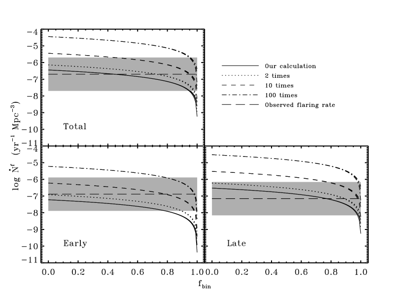
Figure 12: Expected tidal disruption rates of stellar objects by black holes as a function of the fraction of binaries for all (upper), early (lower left), and late (lower right) type galaxies. Solid lines are our calculated flaring rates for spherical galaxies with two-body relaxation. Dotted, short-dashed, and dot-dashed lines are calculated by simply multiplying the solid lines with, respectively, $2$, $10$, and $100$. The long-dashed horizontal lines indicates the best estimates of the flaring rates in real universe and the shaded regions corresponding to an assumed statistical uncertainty of one order magnitude.

If a fraction, $f_{\rm bin}$, of SMBHs in the investigated galaxies are in binary and a fraction $1-f_{\rm bin}$ are single, the expected tidal disruption rate is

$$\dot{N}^{f} = (1-f_{\rm bin})\dot{N}^{f}_{\rm single}+f_{\rm bin}(\dot{N}^{f}_{1}+\dot{N}^{f}_{2})\,.$$ (19)

$\dot{N}^{f}$ as a function of $f_{\rm bin}$ is presented in Figure 12. It shows that $\dot{N}^{f}$ is not sensitive to $q$ unless $f_{\rm bin}\simeq 1$. In § 7 we will use these $f_{\rm bin}-\dot{N}^{f}$ diagrams to constrain $f_{\rm bin}$ for different types of galaxies.

7 DISCUSSION

The hierarchical structure formation model in CDM cosmology predicts that SMBHBs are continuously formed across the merging history of galaxies. Constraining the abundance of SMBHBs among inactive galaxies is essential to test the theoretical models of the dynamic evolution of binary BHs. In this paper we have studied the effect of hard binary BHs on stellar disruption rates, trying to find distinct observational signatures of SMBHBs in galaxy centers. We focus our attention on inactive galaxies which contain the final products of BH mergers so we do not consider the effect of gas on SMBHB evolution.

We have carried out numerical scattering experiments designed for hard SMBHBs to investigate the probability of stellar disruption. Since $r_{t}\ll a_{h}$, in each set of experiments usually a large number of test particles ($N\simeq 10^{7}$) were used to give statistical meaningful results. For solar type stars the test particle approximation should be valid outside $r_{t}$ as long as $E_{0}\ll GM_{12}/a$. In this situation the self-binding energy of a star $\sim Gm_{*}^{2}/r_{*}$ is smaller by a factor $(M_{\bullet}/M_{*})^{2/3}$ than its kinetic energy at $r_{t}$ so the loss of orbital energy due to tidal dissipation is not important. The test particle approximation may be problematic for giant stars because they are much less concentrated and may suffer from mass stripping during their encounters with BHs. This uncertainty could be incorporated into the uncertainty in $r_{g}$. In single BH case the stellar disruption rate is not sensitive to $r_{g}$ if the loss cone is in the diffusive regime but would be proportional to $r_{g}$ if the loss cone is in the pinhole regime (MT99). For binary BHs the loss cone filling rate does not depend on $r_{g}$ but the tidal disruption cross section scales with $r_{g}$ when gravitational focusing is important. Therefore unless the effective $r_{g}$ deviates significantly from our choice $r_{g}=15r_{\odot}$ our results for giant stars would not be qualitatively different.

We find that in binary BH systems the multi-encounter cross sections are greater than the single-encounter ones. This is because binary BHs tend to scatter particles onto temporary bound orbits which enhances the number of star-binary encounters. If a star is only partly disrupted during each close passage from the BHs, multi-flares would be produced occur due to the multi-encounters, which provides a distinct observational signature of SMBHBs. However, we have seen in § 4.1 that the probability of multi-flaring may be extremely low because $r_{t}\ll a$. Even if $r_{t}\sim a$ equation (12) implies that $a/r_{{\rm S}1}\sim M_{8}^{-2/3}$ so gravitational wave radiation would quickly drive the BHs to coalesce, making the multi-flares unlikely. A secondary flare could also be produced if the secondary member of SMBHB captures sufficient debris from the star disrupted by the primary BH, or vise versa. The probability of these events depends on the opening angle of all the spewed debris about the stellar disrupting BH, which needs to be determined by hydrodynamic simulations.

We have shown that the normalized cross sections are not sensitive to the star’s initial binding energy or to the eccentricity of the BH binary, but do depend on the amplitude and orientation of the star’s initial angular momentum. The cross sections presented in Figures 1 and 7, which have been equally averaged over the whole loss cone and over all directions, can be directly used if the loss cone of SMBHB is isotropic and is in the pinhole regime. In the diffusive loss cone limit the stars falling to the binary BHs satisfy $J\gtrsim J_{\rm lc}$. According to Figure 4 the differential tidal disruption cross sections at $J\gtrsim J_{\rm lc}$ are lower than those inside the loss cone, so the mean tidal disruption cross section in the diffusive limit is smaller than those presented in Figures 1 and 7.

We find that the tidal disruption rates in binary BH systems are more than one order of magnitude lower than those in single BH systems. The suppression of stellar disruption rate by SMBHB originates in the low loss cone filling rate in binary BH systems, which results from the stellar cusp destruction due to the hardening of SMBHBs. Even efficient loss cone filling mechanisms are taken into account the contrast between the stellar disruption rates in single and binary BH cases are still prominent in less massive galaxies with $M_{\bullet}\lesssim 10^{8}M_{\odot}$, because the survival of SMBHBs requires that the loss cone filling rate should not exceed a critical value which is proportional to the total BH mass of SMBHB. Our result is qualitatively different from that of Ivanov et al. (2005), who suggested that a SMBHB will enhance the stellar disruption rates. The difference is due to that we are studying a much later evolution stage at which the dense galactic cusps considered by Ivanov et al. have been destroyed during the hardening of SMBHBs. According to the calculation in Y02 binary BHs reach the hard radius in about a dynamic friction timescale of the merging galaxy. So the situation considered by Ivanov et al. (2005) applies for a short period relative to the lifetime of a galaxy. Merritt & Wang (2005) suggested that because loss cone refilling takes time the stellar disruption rate immediately after SMBHB coalescence is significantly below the final steady disruption rate. But this effect is prominent only in massive galaxies with $M_{\bullet}>10^{8}M_{\odot}$, where the relaxation timescale is long. Our result implies that in less massive galaxies the flaring rate could give stringent constraint to the abundance of SMBHB.

In larger galaxies with $M_{\bullet}>10^{8}M_{\odot}$ tidal flares are dominated by disruption of giants. However, their spectral and variable properties may be different from those of solar type stars. A tidal flare is expected to be produced at a scale about $r_{t}$, initially radiating at the Eddington limit $L_{\rm Edd}\simeq 1.3\times 10^{45}(M_{\bullet}/10^{7}M_{\odot})~{}{\rm erg~{}s^{-1}}$ with a thermal spectrum of effective temperature $T_{\rm eff}\simeq[L_{\rm Edd}/(4\pi r_{t}^{2}\sigma)]^{1/4}=2.4\times 10^{5}(r_{*}/r_{\odot})^{-1/2}(m_{*}/M_{\odot})^{1/6}M_{8}^{1/12}~{}{\rm K}$ and decaying on a timescale $t_{\rm flare}\sim\pi GM_{\bullet}(2\Delta E)^{-3/2}\simeq 1.1~{}{\rm yr}(r_{*}/r_{\odot})^{3/2}(m_{*}/M_{\odot})^{-1}M_{8}^{1/2}$, where $\Delta E\sim GM_{\bullet}r_{*}/r_{t}^{2}$ characterizes the span of the binding energy of the debris (Rees, 1988). For solar type stars the spectrum of tidal flare peaks at UV or soft X-ray and the luminosity decays in about $M_{8}^{1/2}$ year. While for giant stars with $r_{*}=15r_{\odot}$ and $m_{*}=m_{\odot}$ the spectrum peaks at optical or UV band and the flare dims on a timescale of about $60M_{8}^{1/2}$ years. Therefore if a UV/X-ray outburst decaying within months to one year is detected in a galaxy with total BH mass much greater than $10^{8}M_{\odot}$ (determined by other observations), it is likely that a less massive secondary SMBH resides in the galactic center. Such event is another signature of SMBHB, though Figure 10 suggests that the frequency of such event is low.

So far six candidate tidal disruption events have been observed in nearby inactive galaxies. Among them, one was observed at $z=0.37$ by the UV telescope GALEX (Gezari et al., 2006) and the rest were discovered in galaxies at $z\lesssim 0.15$ during the one year ROSAT All Sky Survey (RASS) (Komossa, 2002). The Hubble types for the host galaxies of the five RASS flares are not well determined: NGC 5905 is of a SB galaxy and the other four galaxies look like ellipticals (Komossa, 2002). From the observations of RASS Donley et al. (2002) inferred a total flaring rate of $\dot{N}^{f}_{\rm obs}\sim 2\times 10^{-7}~{}{\rm yr^{-1}~{}Mpc^{-3}}$ for all types of galaxies. From the RASS results we can also give a rough estimate of the flaring rates for different types of galaxies: $\dot{N}^{f}_{\rm obs}\sim 1.3\times 10^{-7}~{}{\rm yr^{-1}~{}Mpc^{-3}}$ for early type galaxies and $\dot{N}^{f}_{\rm obs}\sim 7\times 10^{-8}~{}{\rm yr^{-1}~{}Mpc^{-3}}$ for late types. We plot $\dot{N}^{f}_{\rm obs}$ as long-dashed horizontal lines in Figure 12 and the corresponding uncertainties with shaded areas. Because of the poor statistics in $\dot{N}^{f}_{\rm obs}$ and the ill-determination of Hubble types of the host galaxies, the results are highly uncertain.

We did the calculation based on the assumptions that galaxies are spherical and two-body scattering relaxation dominates the loss-cone refilling. However, taking into account more realistic non-spherical stellar distributions and other loss-cone refilling mechanisms besides two-body interaction will probably significantly increase the loss-cone refilling rates in both single and binary SMBH systems. MT99 and Y02 showed that taking into account axisymmetric stellar distribution will increase the loss cone refilling rates by a factor of $2$ for both single SMBHs and hard SMBHBs. The loss cone refilling rates in triaxial galaxies are slightly higher than those in axisymmetric ones if the triaxiality is less than $0.1$ but can be two orders of magnitude higher if the triaxiality is more extreme (Y02; Merritt & Poon, 2004). Resonant relaxation would increase the loss cone refilling rates by a factor of $2-10$ relative to those in the case of two-body relaxation, depending on the eccentricities of stellar orbits (Rauch & Tremaine, 1996; Rauch & Ingalls, 1998; Gürkan & Hopman, 2007). To calculate the tidal disruption rates by taking into account the above physical processes is out of the scope of this paper. To illustrate the effects of increased loss-cone refilling rates and tidal disruption rates on the estimated fraction of binary BHs, $f_{\rm bin}$, we simply multiply our calculated stellar disruption rates $\dot{N}^{f}$ by $2$, $10$, and $100$ and plot the results in Figure 12. In Figure 12, the intersections of long-dashed and solid lines give the lower limit to $f_{\rm bin}$, while the intersections of long-dashed and dot-dashed lines roughly give the upper limits. When all types of galaxies are considered, binary fraction $f_{\rm bin}$ is between $0.4$ and $1.0$. For early type galaxies, the solid lines do not intersect the long-dashed line, implying that other loss-cone filling mechanisms in addition to two-body relaxation should also be important. For late type galaxies, Figure 12 suggests a binary fraction $f_{\rm bin}\sim 75\%$ and that extreme triaxiality may not be common, otherwise the current observation would imply an extremely high fraction of SMBHBs. We would like to note that the constraints on $f_{\rm bin}$ are very uncertain due to the large uncertainty in the current $\dot{N}^{f}_{\rm obs}$. Detection of more candidate tidal disruption events is needed to give better constraints on $f_{\rm bin}$ and on the dominant loss-cone filling mechanisms in different types of galaxies.

The non-detection of X-ray or UV flares in dwarf galaxies seems inconsistent with the calculated high flaring rates. The discrepancy may be due to (1) a lack of sufficient sensitivity in current surveys, (2) the continuous and steady accretion of stellar debris onto IMBHs during successive tidal disruption events (Milosavljević et al., 2006), or (3) a lack of IMBHs in the centers of dwarf galaxies. Future X-ray and UV surveys with improved sensitivity and angular resolution would help constraining the fraction of IMBHs in galaxy centers and give interesting implications to the formation and the merging history of IMBHs (Volonteri et al., 2003; Volonteri, 2007).

8 CONCLUSIONS

To investigate whether SMBHBs are ubiquitous in nearby inactive galaxies or coalesce rapidly in galaxy mergers, we have studied the tidal disruption rates of stellar objects in both single and binary SMBH systems. We have calculated the interaction cross sections between hard SMBHBs and intruding stars by carrying out intensive numerical scattering experiments with typically $10^{7}$ particles, taking into account the initial binding energy and angular momentum of particle, the eccentricity of the orbit of SMBHB, and including general relativistic effects. We have also derived empirical formulae for the relativistic cross sections, which can be applied to SMBHBs with a wide range of semimajor axis and todal BH mass.

We have calculated the rate of loss cone refilling due to two-body relaxation for a sample of $51$ nearby galaxies, assuming that each galaxy is spherical. The steady loss cone filling rates in binary BH systems would be significantly suppressed due to the three-body interaction between SMBHBs and stars passing by. We have calculated the tidal disruption rates respectively for single and binary SMBHs by combining the loss cone filling rates and the tidal disruption cross sections. We find that the tidal disruption rate in SMBHB systems is more than one order of magnitude lower than that in single SMBH systems. For galaxies with BHs more massive than $10^{8}M_{\odot}$, a UV/X-ray flare at galactic center decaying within one year provides strong evidence of a secondary BH, although the probability of such events is low.

Finally we have calculated the flaring rates in local universe using the BH mass function given in the literature. The comparison of the calculated flaring rates and the preliminary results from current X-ray surveys could not yet tell whether SMBHBs are ubiquitous in local universe. Future UV/X-ray surveys with improved sensitivity and duration are needed.

References

- Armitage & Natarajan (2002) Armitage, P. J. & Natarajan, P., 2002, ApJ, 567, L9
- Begelman et al. (1980) Begelman, M. C., Blandford, R. D., & Rees, M. J., 1980, Nature, 287, 307
- Berczik et al. (2006) Berczik, P., Merritt, D., Spurzem, R., & Bischof, H.-P., 2006, ApJ, 642, L21
- Bond, Arnett & Carr (1984) Bond, J. R., Arnett, W. D., & Carr, B. J., 1984, ApJ, 280, 825
- Chatterjee et al. (2003) Chatterjee, P., Hernquist, L., Loeb, A., 2003, ApJ, 592, 32
- Cohn & Kulsrud (1978) Cohn, H. & Kulsrud, R. M., 1978, ApJ, 226, 1087
- Croton et al. (2006) Croton, D. J. et al., 2006, MNRAS, 365, 11
- Donley et al. (2002) Donley, J. L., Brandt, W. N., Eracleous, M., & Boller, T., 2002, AJ, 124, 1308
- Escala et al. (2005) Escala, A., Larson, R. B., Coppi, P. S., & Mardones, D., 2005, ApJ, 630, 152
- Ferrarese & Ford (2005) Ferrarese, L. & Ford, H., 2005, SSRv, 116, 523
- Ferrarese & Merritt (2000) Ferrarese, L. & Merritt, D., 2000, ApJ, 539, L9
- Gaskell (1985) Gaskell, C. M., 1985, Nature, 315, 386
- Gebhardt et al. (2000) Gebhardt, K. et al., 2000, ApJ, 539, L13
- Gezari et al. (2006) Gezari, S. et al., 2006, ApJ, 653, L25
- Gould & Rix (2000) Gould, A. & Rix, H. W., 2000, ApJ, 532, L29
- Gürkan & Hopman (2007) Gürkan, M. A. & Hopman C., 2007, MNRAS, 379, 1083
- Haehnelt & Kauffmann (2002) Haehnelt, M. G. & Kauffmann, G., 2002, ApJ, 336, 61L
- Hairer et al. (1987) Hairer, E., Norsett, S. P., & Wanner, G., 1987, Solving Ordinary Differential Equations I (1st ed.; Berlin: Springer-Verlag)
- Halpern et al. (2004) Halpern, J. P., Gezari, S. & Komossa, S., 2004, ApJ, 604, 572
- Häring & Rix (2004) Häring, N. & Rix, H.-W., 2004, ApJ, 604, 89L
- Hernquist & Mihos (1995) Hernquist, L. & Mihos, J. C., 1995, ApJ, 448, 41
- Hills (1975) Hills, J. G., 1975, ApJ, 254, 295
- Hills (1983) Hills, J. G., 1983, ApJ, 88, 1857
- Hopkins et al. (2006) Hopkins, P. F., Somerville, R. S., Hernquist, L., Cox, T. J., Robertson, B., & Li, Y., 2006, ApJ, 652, 864
- Hut (1983) Hut, P., 1983, ApJ, 272, L29
- Ivanov & Chernyakova (2006) Ivanov, P. B. & Chernyakova, M. A., 2006, A&A, 448, 843
- Ivanov et al. (1999) Ivanov, P. B., Papaloizou, J. C. B., & Polnrev, A. G., 1999, MNRAS, 307, 79
- Ivanov et al. (2005) Ivanov, P. B., Polnarev, A. G., & Saha, P., 2005, MNRAS, 358, 1361
- Kauffmann & Haehnelt (2000) Kauffmann, G. & Haehnelt, M. G., 2000, MNRAS, 311, 576
- Kazantzidis et al. (2005) Kazantzidis, S. et al., 2005, ApJ, 623, L67
- Komossa (2002) Komossa, S., 2002, Rev. Mod. Astron., 15, 27 (astro-ph/0209007)
- Komossa (2006) Komossa, S., 2006, MmSAI, 77, 733
- Komossa & Greiner (1999) Komossa, S. & Greiner, J., 1999, A&A, 349, L45
- Komossa et al. (2004) Komossa, S., Halpern, J., Schartel, N., Hasinger, G., Santos-Lleo, M., & Predehl, P., 2004, ApJ, 603, L17
- Liu (2004) Liu F. K., 2004, MNRAS, 347, 1357
- Liu & Chen (2007) Liu, F. K. & Chen, X., 2007, ApJ, 671, no. 2 (astro-ph/0705.1077)
- Liu et al. (1997) Liu, F. K., Liu, B. F., & Xie, G. Z., 1997, A&AS, 123, 569
- Liu & Wu (2002) Liu, F. K. & Wu, X. B., 2002, A&A, 388, L48
- Liu et al. (2003) Liu, F. K., Wu, X. B., & Cao, S. L., 2003, MNRAS, 340, 411
- Liu et al. (1995) Liu, F. K., Xie, G. Z., & Bai, J. M., 1995, A&A, 295, 1
- Liu et al. (2006) Liu, F. K., Zhao, G., & Wu, X. B., 2006, ApJ, 650, 749
- Lu et al. (2007) Lu, Y., Yu, Q., & Lin, D. N. C., 2007, ApJ, 666, L89
- Marconi et al. (2004) Marconi, A., Risaliti, G., Gilli, R., Hunt, L. K., Maiolino, R., & Salvati, M., 2004, MNRAS, 351, 169
- Magorrian et al. (1998) Magorrian, J. et al., 1998, AJ, 115, 2285
- Magorrian & Tremaine (1999) Magorrian, J. & Tremaine, S., 1999, MNRAS, 309, 447 (MT99)
- McLure & Dunlop (2002) McLure, R. J. & Dunlp, J. S., 2002, MNRAS, 331, 795
- Merritt (2006) Merritt, D., 2006, ApJ, 648, 976
- Merritt & Ekers (2002) Merritt, D. & Ekers, R. D., 2002, Sci, 297, 1310
- Merritt & Milosavljević (2005) Merritt, D. & Milosavljević, M., 2005, Liv. Rev. Rel., 8, 8
- Merritt & Poon (2004) Merritt, D. & Poon, M. Y., 2004, ApJ, 606, 788
- Merritt & Wang (2005) Merritt, D. & Wang, J.-X., 2005, ApJ, 621, L101
- Milosavljević & Merritt (2001) Milosavljević, M. & Merritt, D., 2001, ApJ, 563, 34
- Milosavljević & Merritt (2003) Milosavljević, M. & Merritt, D., 2003, ApJ, 596, 860
- Milosavljević et al. (2006) Milosavljević, M., Merritt, D. & Ho, L. C., 2006, ApJ, 652, 120
- Nolthenus & Katz (1983) Nolthenus, R. A. & Katz, J. I., 1983, ApJ, 269, 297
- Ostorero et al. (2004) Ostorero, L., Villata, M., & Raiteri, C. M., 2004, A&A, 419, 913
- Paczyński & Witta (1980) Paczyński, B. & Witta, P. J., 1980, A&A, 88,23
- Peters (1964) Peters, P. C., 1964, Phys. Rev. B, 136, 1224
- Quinlan (1996) Quinlan, G. D., 1996, New A, 1, 35, (Q96)
- Raiteri et al. (2001) Raiteri, C. M. et al., 2001, A&A, 377, 396
- Rauch & Ingalls (1998) Rauch, K. P. & Ingalls, B., 1998, MNRAS, 299, 1231
- Rauch & Tremaine (1996) Rauch, K. P. & Tremaine, S., 1996, New A, 1, 149
- Rees (1988) Rees, M. J., 1988, Nature, 333, 523
- Richstone et al. (1998) Richstone, D. O. et al. 1998, Nature, 395, 14
- Romero et al. (2000) Romero, G. E., Chajet, L., Abraham, Z. & Fan, J. H., 2000, A&A, 360, 57
- Sillanpää et al. (1988) Sillanpää, A., Haarala, S., Valtonen, M. J., Sundelius, B., & Byrd, G. G., 1988, ApJ, 325, 628
- Sesana et al. (2006) Sesana, A., Haardt, F., & Madau, P., 2006, ApJ, 651, 392
- Springel et al. (2005) Springel, V. et al., 2005, Nature, 435, 629
- Syer & Ulmer (1999) Syer, D. & Ulmer, A., 1999, MNRAS, 306, 35
- Tremaine et al. (2002) Tremaine, S. et al., 2002, ApJ, 574, 740
- Ulmer (1999) Ulmer, A., 1999, ApJ, 514, 180
- Valtaoja et al. (2000) Valtaoja, E., Teräsranta, H., Tornikoshi, M., Sillanpää, A., Aller, M. F., Aller, H. D. & Hughes, P. A., 2000, ApJ, 531, 744
- Villata & Raiteri (1999) Villata, M. & Raiteri, C. M., 1999, A&A, 347, 30
- Volonteri (2007) Volonteri, V., 2007, ApJ, 663, L1
- Volonteri et al. (2003) Volonteri, M., Haardt, F., & Madau, P., 2003, ApJ, 582, 559
- Wang & Merritt (2004) Wang, J.-X. & Merritt, D., 2004, ApJ, 600, 149
- Yu (2002) Yu, Q., 2002, MNRAS, 331, 935 (Y02)
- Yu & Tremaine (2002) Yu, Q. & Tremaine, S., 2002, MNRAS, 335, 965
- Zier (2005) Zier, C., 2005, MNRAS, 364, 583