Incremental magnetoelastic deformations,
with application to surface instability

Abstract

In this paper the equations governing the deformations of infinitesimal (incremental) disturbances superimposed on finite static deformation fields involving magnetic and elastic interactions are presented. The coupling between the equations of mechanical equilibrium and Maxwell’s equations complicates the incremental formulation and particular attention is therefore paid to the derivation of the incremental equations, of the tensors of magnetoelastic moduli and of the incremental boundary conditions at a magnetoelastic/vacuum interface.

The problem of surface stability for a solid half-space under plane strain with a magnetic field normal to its surface is used to illustrate the general results. The analysis involved leads to the simultaneous resolution of a bicubic and vanishing of a $7\times 7$ determinant. In order to provide specific demonstration of the effect of the magnetic field, the material model is specialized to that of a “magnetoelastic Mooney-Rivlin solid”. Depending on the magnitudes of the magnetic field and the magnetoelastic coupling parameters, this shows that the half-space may become either more stable or less stable than in the absence of a magnetic field.

1 Introduction

One of the main reasons for industrial interest in rubber-like materials resides in their ability to dampen vibrations and to absorb shocks. This paper is concerned with an extension of the nonlinear elasticity theory adopted for describing the properties of these materials to incorporate nonlinear magnetoelastic effects so as to embrace a class of solids referred to as magneto-sensitive (MS) elastomers. These “smart” elastomers typically consist of an elastomeric matrix (rubber, silicon, for example) with a distribution of ferrous particles (with a diameter of the order of 1–5 micrometers) within their bulk. They are sensitive to magnetic fields in that they can deform significantly under the action of magnetic fields alone without mechanical loading, a phenomenon known as magnetostriction. As a result, their mechanical damping abilities can be controlled by applying suitable magnetic fields. This coupling between elasticity and magnetism was probably first observed by Joule in 1847 when he noticed that a sample of iron changed its length when magnetized.

In general, the physical properties of magnetoelastic materials depend on factors such as the choice of magnetizable particles, their volume fraction within the bulk, the choice of the matrix material, the chemical processes of curing, etc.; see [1] for details, and also [2] for an experimental study on a magneto-sensitive elastomer.

The coupling between magnetism and nonlinear elasticity has generated much interest over the last $50$ years or so, as illustrated by the works of Truesdell and Toupin [3], Brown [4], Yu and Tang [5], Maugin [6], Eringen and Maugin [7], Kovetz [8], and others. The corresponding engineering applications are more recent (see Jolly et al. [9], or Dapino [10], for instance) and have generated renewed impetus in theoretical modelling (see, for example, Dorfmann and Brigadnov [11]; Dorfmann and Ogden [12]); Kankanala and Triantafyllidis [13]. Here, we derive the (linearized) equations governing incremental effects in a magnetoelastic solid subject to finite deformation in the presence of a magnetic field. These equations are then used to examine the problem of surface stability of a homogeneously pre-strained half-space subject to a magnetic field normal to its (plane) boundary. Related works on this subject include the studies of McCarthy [14], van de Ven [15], Boulanger [16, 17], Maugin [18], Carroll and McCarthy [19] and Das et al. [20].

We adopt the formulation of Dorfmann and Ogden [12] as the starting point for the derivation of the incremental equations. This involves a total stress tensor and a modified strain energy function or total energy function, which enable the constitutive law for the stress to be written in a form very similar to that in standard nonlinear elasticity theory. The coupled governing equations then have a simple structure. We summarize these equations in Section 2. For incompressible isotropic magnetoelastic materials the energy density is a function of five invariants, which we denote here by $I_{1}$ and $I_{2}$, the first two principal invariants of the Cauchy-Green deformation tensors, and $I_{4}$, $I_{5}$, $I_{6}$, three invariants involving a Cauchy-Green tensor and the magnetic induction vector. This formulation is similar in structure to that associated with transversely isotropic elastic solids (see Spencer [21]). The general incremental equations of nonlinear magnetoelasticity are then derived in Section 3. Therein we define the various magnetoelastic ‘moduli’ tensors and provide general incremental boundary conditions. Care is needed in deriving the boundary equations since the Lagrangian fields in the solid and the Eulerian fields in the vacuum must be reconciled.

Section 4 provides a brief summary of the basic equations associated with the pure homogeneous plane strain of a half-space of magnetoelastic material with a magnetic field normal to its boundary. In Section 5, the general incremental equations are applied to the analysis of surface stability. Not surprisingly, the resulting bifurcation criterion is a complicated equation, even when the pre-stress corresponds to plane strain and the magnetic induction vector is aligned with a principal direction of strain, as is the case here. The bifurcation equation comes from the vanishing of the determinant of a $7\times 7$ matrix, which must be solved simultaneously with a bicubic equation. To present a tractable example, we therefore focus on a “Mooney-Rivlin magnetoelastic solid” for which the total energy function is linear in the invariants $I_{1}$, $I_{2}$, $I_{4}$, and $I_{5}$. Of course, these invariants are nonlinear in the deformation and the theory remains highly nonlinear. The bicubic then factorizes and a complete analytical resolution follows. In addition to the two elastic Mooney-Rivlin parameters (material constants), the material model involves two magnetoelastic coupling parameters. The stability behaviour of the half-space depends crucially on the values of these coupling parameters and also on the magnitude of the magnetic field. In particular, a judicious choice of parameters can stabilize the half-space relative to the situation in the absence of a magnetic field. Equally, the half-space can become de-stabilized for different choices of the parameters. Thus, even this very simple model illustrates the possible complicated nature of the magnetoelastic coupling in the nonlinear regime.

2 The equations of nonlinear magnetoelasticity

In this section the equations for nonlinear magnetoelastic deformations, as developed by Dorfmann and Ogden [12, 22, 23, 24], are summarized for subsequent use in the derivation of the incremental equations.

We consider a magnetoelastic body in an undeformed configuration $\mathcal{B}_{0}$, with boundary $\partial\mathcal{B}_{0}$. A material point within the body in that configuration is identified by its position vector $\boldsymbol{X}$. By the combined action of applied mechanical loads and magnetic fields, the material is then deformed from $\mathcal{B}_{0}$ to the configuration $\mathcal{B}$, with boundary $\partial\mathcal{B}$, so that the particle located at $\boldsymbol{X}$ in $\mathcal{B}_{0}$ now occupies the position $\boldsymbol{x}=\boldsymbol{\chi}(\boldsymbol{X})$ in the deformed configuration $\mathcal{B}$. The function $\boldsymbol{\chi}$ describes the static deformation of the body and is a one-to-one, orientation-preserving mapping with suitable regularity properties. The deformation gradient tensor $\boldsymbol{F}$ relative to $\mathcal{B}_{0}$ is defined by $\boldsymbol{F}=\text{Grad}\boldsymbol{\chi}$, $F_{i\alpha}=\partial x_{i}/\partial X_{\alpha}$, Grad  being the gradient operator in $\mathcal{B}_{0}$. The magnetic field vector in $\mathcal{B}$ is denoted $\boldsymbol{H}$, the associated magnetic induction vector by $\boldsymbol{B}$ and the magnetization vector by $\boldsymbol{M}$.

To avoid a conflict of standard notations, the Cauchy-Green tensors are represented here by lower case characters; thus, the left and right Cauchy-Green tensors are $\boldsymbol{b}=\boldsymbol{FF}^{t}$ and $\boldsymbol{c}=\boldsymbol{F}^{t}\boldsymbol{F}$, respectively, where ^t denotes the transpose. The Jacobian of the deformation gradient is $J=\det\boldsymbol{F}$, and the usual convention $J>0$ is adopted.

2.1 Mechanical equilibrium

Conservation of the mass for the material is here expressed as

$$J\rho=\rho_{0},$$ (2.1)

where $\rho_{0}$ and $\rho$ are the mass densities in the configurations $\mathcal{B}_{0}$ and $\mathcal{B}$, respectively. For an incompressible material, $J=1$ is enforced so that $\rho=\rho_{0}$.

The equilibrium equation in the absence of mechanical body forces, is given in Eulerian form by

$$\mbox{div\hskip 1.0pt}\boldsymbol{\tau}=\boldsymbol{0},$$ (2.2)

where $\boldsymbol{\tau}$ is the total Cauchy stress tensor, which is symmetric, and div  is the divergence operator in $\mathcal{B}$. The total nominal stress tensor $\boldsymbol{T}$ is then defined by

$$\boldsymbol{T}=J\boldsymbol{F}^{-1}\boldsymbol{\tau},$$ (2.3)

so that the Lagrangian counterpart of the equilibrium equation (2.2) is

$$\mbox{Div\hskip 1.0pt}\boldsymbol{T}=\boldsymbol{0},$$ (2.4)

Div  being the divergence operator in $\mathcal{B}_{0}$.

Let $\boldsymbol{N}$ denote the unit outward normal vector to $\partial\mathcal{B}_{0}$ and $\boldsymbol{n}$ the corresponding unit normal to $\partial\mathcal{B}$. These are related by Nanson’s formula $\boldsymbol{n}{\rm d}a=J\boldsymbol{F}^{-t}\boldsymbol{N}{\rm d}A$, where ${\rm d}A$ and ${\rm d}a$ are the associated area elements. The traction on the area element in $\partial\mathcal{B}$ may be written $\boldsymbol{\tau}\boldsymbol{n}{\rm d}a$ or as $\boldsymbol{T}^{t}\boldsymbol{N}{\rm d}A$. A traction boundary condition might therefore be expressed in the form

$$\boldsymbol{T}^{t}\boldsymbol{N}=\boldsymbol{t}_{\text{a}},$$ (2.5)

where $\boldsymbol{t}_{\text{a}}$ is the applied traction per unit reference area. If this is independent of the deformation then the traction is said to be a dead load.

2.2 Magnetic balance laws

In the Eulerian description, Maxwell’s equations in the absence of time dependence, free charges and free currents reduce to

$$\mbox{div\hskip 1.0pt}\boldsymbol{B}=0,\quad\mbox{curl\hskip 1.0pt}\boldsymbol{H}=\boldsymbol{0},$$ (2.6)

which hold both inside and outside a magnetic material, where curl  relates to $\mathcal{B}$. Thus, $\boldsymbol{B}$ and $\boldsymbol{H}$ can be regarded as fundamental field variables. A third vector field, the magnetization, when required, can be defined by the standard relation

$$\boldsymbol{B}=\mu_{0}(\boldsymbol{H}+\boldsymbol{M}).$$ (2.7)

We shall not need to make explicit use of the magnetization in this paper.

Associated with the equations (2.6) are the boundary continuity conditions

$$(\boldsymbol{B}-\boldsymbol{B}^{\star})\cdot\boldsymbol{n}=0,\quad(\boldsymbol{H}-\boldsymbol{H}^{\star})\times\boldsymbol{n}=\boldsymbol{0},$$ (2.8)

wherein $\boldsymbol{B}$ and $\boldsymbol{H}$ are the fields in the material and $\boldsymbol{B}^{\star}$ and $\boldsymbol{H}^{\star}$ the corresponding fields exterior to the material, but in each case evaluated on the boundary $\partial\mathcal{B}$.

Lagrangian counterparts of $\boldsymbol{B}$ and $\boldsymbol{H}$, denoted $\boldsymbol{B}_{l}$ and $\boldsymbol{H}_{l}$, respectively, are defined by

$$\boldsymbol{B}_{l}=J\boldsymbol{F}^{-1}\boldsymbol{B},\quad\boldsymbol{H}_{l}=\boldsymbol{F}^{t}\boldsymbol{H},$$ (2.9)

and in terms of these quantities equations (2.6) become

$$\mbox{Div\hskip 1.0pt}\boldsymbol{B}_{l}=0,\quad\mbox{Curl\hskip 1.0pt}\boldsymbol{H}_{l}=\boldsymbol{0},$$ (2.10)

where Curl  is the curl operator in $\mathcal{B}_{0}$. We note in passing that a Lagrangian counterpart of $\boldsymbol{M}$ may also be defined, one possibility being $\boldsymbol{M}_{l}=\boldsymbol{F}^{t}\boldsymbol{M}$.

The boundary conditions (2.8) can also be expressed in Lagrangian form, namely

$$(\boldsymbol{B}_{l}-J\boldsymbol{F}^{-1}\boldsymbol{B}^{\star})\cdot\boldsymbol{N}=0,\quad(\boldsymbol{H}_{l}-\boldsymbol{F}^{t}\boldsymbol{H}^{\star})\times\boldsymbol{N}=\boldsymbol{0},$$ (2.11)

evaluated on the boundary $\partial\mathcal{B}_{0}$.

2.3 Constitutive equations

There are many possible ways to formulate constitutive laws for magnetoelastic materials based on different choices of the independent magnetic variable and the form of energy function. For present purposes it is convenient to use a formulation involving a ‘total energy function’, or ‘modified free energy function’, which is denoted here by $\Omega$, following Dorfmann and Ogden [12]. This is defined per unit reference volume and is a function of $\boldsymbol{F}$ and $\boldsymbol{B}_{l}$: $\Omega(\boldsymbol{F},\boldsymbol{B_{l}})$. This leads to the very simple expressions

$$\boldsymbol{T}=\frac{\partial\Omega}{\partial\boldsymbol{F}},\quad\boldsymbol{H}_{l}=\frac{\partial\Omega}{\partial\boldsymbol{B}_{l}}$$ (2.12)

for a magnetoelastic material without internal mechanical constraints, and

$$\boldsymbol{T}=\frac{\partial\Omega}{\partial\boldsymbol{F}}-p\boldsymbol{F}^{-1},\quad\boldsymbol{H}_{l}=\frac{\partial\Omega}{\partial\boldsymbol{B}_{l}}$$ (2.13)

for an incompressible material, where $p$ is a Lagrange multiplier associated with the constraint $\det\boldsymbol{F}=1$. Note that the expression for $\boldsymbol{H}_{l}$ is unchanged except that now $\det\boldsymbol{F}=1$ in $\Omega$.

The Eulerian counterparts of the above equations are

$$\boldsymbol{\tau}=J^{-1}\boldsymbol{F}\frac{\partial\Omega}{\partial\boldsymbol{F}},\quad\boldsymbol{H}=\boldsymbol{F}^{-t}\frac{\partial\Omega}{\partial\boldsymbol{B}_{l}}$$ (2.14)

for an unconstrained material, where $\boldsymbol{F}^{-t}=(\boldsymbol{F}^{-1})^{t}$, and

$$\boldsymbol{\tau}=\boldsymbol{F}\frac{\partial\Omega}{\partial\boldsymbol{F}}-p\boldsymbol{I},\quad\boldsymbol{H}=\boldsymbol{F}^{-t}\frac{\partial\Omega}{\partial\boldsymbol{B_{l}}},$$ (2.15)

where $\boldsymbol{I}$ is the identity tensor. We emphasize that the first equation in each of (2.12)–(2.15) has exactly the same form as for a purely elastic material in the absence of a magnetic field.

2.4 Isotropic magnetoelastic materials

In general the mechanical properties of magnetoelastic elastomers have features that are similar to those of transversely isotropic materials. During the curing process a preferred direction is ’frozen in’ to the material if the curing is done in the presence of a magnetic field, which aligns the magnetic particles. If cured without a magnetic field then the distribution of particles is essentially random and the resulting magnetoelastic response is isotropic. We focus on the latter case here for simplicity, but the corresponding analysis for the more general case follows the same pattern, albeit more complicated algebraically. A general constitutive theory for the former situation has been developed by Bustamante and Ogden [25] and applied to some simple problems. For isotropic materials, the energy function $\Omega$ depends only on $\boldsymbol{c}$ and $\boldsymbol{B}_{l}\otimes\boldsymbol{B}_{l}$, through the six invariants

$$I_{1}=\text{tr}\,\boldsymbol{c}, I_{2}=\tfrac{1}{2}\left[(\text{tr}\,\boldsymbol{c})^{2}-(\text{tr}\,\boldsymbol{c}^{2})\right], I_{3}=\det\boldsymbol{c}=J^{2},$$

$$I_{4}=\boldsymbol{B}_{l}\cdot\boldsymbol{B}_{l}, I_{5}=(\boldsymbol{c\,B}_{l})\cdot\boldsymbol{B}_{l}, I_{6}=(\boldsymbol{c}^{2}\,\boldsymbol{B}_{l})\cdot\boldsymbol{B}_{l}.$$ (2.16)

For incompressible materials, $I_{3}=1$ and only the five invariants $I_{1}$, $I_{2}$, $I_{4}$, $I_{5}$, and $I_{6}$ remain. The total stress tensor $\boldsymbol{\tau}$ is then expressed as

$$\boldsymbol{\tau}=-p\boldsymbol{I}+2\Omega_{1}\boldsymbol{b}+2\Omega_{2}(I_{1}\boldsymbol{b}-\boldsymbol{b}^{2})+2\Omega_{5}\boldsymbol{B}\otimes\boldsymbol{B}+2\Omega_{6}(\boldsymbol{B}\otimes\boldsymbol{bB}+\boldsymbol{bB}\otimes\boldsymbol{B}),$$ (2.17)

where $\Omega_{i}=\partial\Omega/\partial I_{i}$, and the total nominal stress tensor $\boldsymbol{T}$ as

$$\boldsymbol{T}=-p\boldsymbol{F}^{-1}+2\Omega_{1}\boldsymbol{F}^{t}+2\Omega_{2}(I_{1}\boldsymbol{F}^{t}-\boldsymbol{F}^{t}\boldsymbol{b})\\ +2\Omega_{5}\boldsymbol{B}_{l}\otimes\boldsymbol{B}+2\Omega_{6}(\boldsymbol{B}_{l}\otimes\boldsymbol{bB}+\boldsymbol{F}^{t}\boldsymbol{B}\otimes\boldsymbol{B}).$$ (2.18)

Finally, the magnetic field vector $\boldsymbol{H}$ is found from (2.15)₂ as

$$\boldsymbol{H}=2(\Omega_{4}\boldsymbol{b}^{-1}\boldsymbol{B}+\Omega_{5}\boldsymbol{B}+\Omega_{6}\boldsymbol{bB}),$$ (2.19)

and its Lagrangian counterpart is

$$\boldsymbol{H}_{l}=2(\Omega_{4}\boldsymbol{B}_{l}+\Omega_{5}\boldsymbol{c}\boldsymbol{B}_{l}+\Omega_{6}\boldsymbol{c}^{2}\boldsymbol{B}_{l}).$$ (2.20)

2.5 Outside the material

In vacuum, there is no magnetization and the standard relation (2.7) reduces to

$$\boldsymbol{B}^{\star}=\mu_{0}\boldsymbol{H}^{\star},$$ (2.21)

where the star is again used to denote a quantity exterior to the material. Also, the stress tensor $\boldsymbol{\tau}$ is now the Maxwell stress $\boldsymbol{\tau}^{\star}$, given by

$$\boldsymbol{\tau}^{\star}=\mu_{0}^{-1}[\boldsymbol{B}^{\star}\otimes\boldsymbol{B}^{\star}-\tfrac{1}{2}(\boldsymbol{B}^{\star}\cdot\boldsymbol{B}^{\star})\boldsymbol{I}],$$ (2.22)

which, since $\mbox{div\hskip 1.0pt}\boldsymbol{B}^{\star}=0$ and $\mbox{curl\hskip 1.0pt}\boldsymbol{B}^{\star}=\boldsymbol{0}$, satisfies $\mbox{div\hskip 1.0pt}\boldsymbol{\tau}^{*}=\boldsymbol{0}$.

3 Incremental equations

3.1 Increments within the material

Suppose now that both the magnetic field and, within the material, the deformation undergo incremental changes (which are denoted by superposed dots). Let $\boldsymbol{\dot{F}}$ and $\boldsymbol{\dot{B}}_{l}$ be the increments in the independent variables $\boldsymbol{F}$ and $\boldsymbol{B}_{l}$. It follows from (2.12) that the increment $\boldsymbol{\dot{T}}$ in $\boldsymbol{T}$ and the increment $\boldsymbol{\dot{H}}_{l}$ in $\boldsymbol{H}_{l}$ are given in the form

$$\boldsymbol{\dot{T}}=\boldsymbol{\mathcal{A}}\boldsymbol{\dot{F}}+\boldsymbol{\Gamma}\boldsymbol{\dot{B}}_{l},\quad\boldsymbol{\dot{H}}_{l}=\boldsymbol{\Gamma}\boldsymbol{\dot{F}}+\boldsymbol{\mathcal{K}}\boldsymbol{\dot{B}}_{l},$$ (3.1)

where $\boldsymbol{\mathcal{A}}$, $\boldsymbol{\Gamma}$ and $\boldsymbol{\mathcal{K}}$ are, respectively, fourth-, third- and second-order tensors, with components defined by

$$\mathcal{A}_{\alpha i\beta j}=\frac{\partial^{2}\Omega}{\partial F_{i\alpha}\partial F_{j\beta}},\quad\Gamma_{\alpha i\beta}=\frac{\partial^{2}\Omega}{\partial F_{i\alpha}\partial B_{l_{\beta}}}=\frac{\partial^{2}\Omega}{\partial B_{l_{\beta}}\partial F_{i\alpha}},\quad\mathcal{K}_{\alpha\beta}=\frac{\partial^{2}\Omega}{\partial B_{l_{\alpha}}\partial B_{l_{\beta}}}.$$ (3.2)

We refer to these tensors as magnetoelastic moduli tensors. We note the symmetries

$$\mathcal{A}_{\alpha i\beta j}=\mathcal{A}_{\beta j\alpha i},\quad\mathcal{K}_{\alpha\beta}=\mathcal{K}_{\beta\alpha},$$ (3.3)

and observe that $\boldsymbol{\Gamma}$ has no such indicial symmetry. The products in (3.1) are defined so that, in component form, we have

$$\dot{T}_{\alpha i}=\mathcal{A}_{\alpha i\beta j}\dot{F}_{j\beta}+\Gamma_{\alpha i\beta}\dot{B}_{l_{\beta}},\quad\dot{H}_{l_{\alpha}}=\Gamma_{\beta i\alpha}\dot{F}_{i\beta}+\mathcal{K}_{\alpha\beta}\dot{B}_{l_{\beta}}.$$ (3.4)

For an unconstrained isotropic material, $\Omega$ is a function of the six invariants $I_{1},I_{2},I_{3},I_{4},I_{5},I_{6}$, and the expressions (3.2) can be expanded in the forms

$$\mathcal{A}_{\alpha i\beta j}=\sum_{m=1,\,m\neq 4}^{6}\sum_{n=1,\,n\neq 4}^{6}\Omega_{mn}\frac{\partial I_{n}}{\partial F_{i\alpha}}\frac{\partial I_{m}}{\partial F_{j\beta}}+\sum_{n=1,\,n\neq 4}^{6}\Omega_{n}\frac{\partial^{2}I_{n}}{\partial F_{i\alpha}\partial F_{j\beta}},$$

$$\Gamma_{\alpha i\beta}=\sum_{m=4}^{6}\sum_{n=1,\,n\neq 4}^{6}\Omega_{mn}\frac{\partial I_{m}}{\partial B_{l_{\beta}}}\frac{\partial I_{n}}{\partial F_{i\alpha}}+\sum_{n=5}^{6}\Omega_{n}\frac{\partial^{2}I_{n}}{\partial F_{i\alpha}\partial B_{l_{\beta}}},$$

$$\mathcal{K}_{\alpha\beta}=\sum_{m=4}^{6}\sum_{n=4}^{6}\Omega_{mn}\frac{\partial I_{m}}{\partial B_{l_{\alpha}}}\frac{\partial I_{n}}{\partial B_{l_{\beta}}}+\sum_{n=4}^{6}\Omega_{n}\frac{\partial^{2}I_{n}}{\partial B_{l_{\alpha}}\partial B_{l_{\beta}}},$$ (3.5)

where $\Omega_{n}=\partial\Omega/\partial I_{n}$, $\Omega_{mn}=\partial^{2}\Omega/\partial I_{m}\partial I_{n}$. Expressions for the first and second derivatives of $I_{n},\,n=1,\dots,6$, are given in the Appendix.

For an incompressible material, $\boldsymbol{T}$ is given by (2.13)₁ and its increment is then

$$\boldsymbol{\dot{T}}=\boldsymbol{\mathcal{A}}\boldsymbol{\dot{F}}+\boldsymbol{\Gamma}\boldsymbol{\dot{B}}_{l}-\dot{p}\boldsymbol{F}^{-1}+p\boldsymbol{F}^{-1}\boldsymbol{\dot{F}}\boldsymbol{F}^{-1},$$ (3.6)

which replaces (3.1) in this case. On the other hand, $\boldsymbol{H}_{l}$ is still given by (2.12)₂ and its increment is unaffected by the constraint of incompressibility, except, of course, since $\Omega$ is now independent of $I_{3}=1$, the summations in equations (3.5) omit $m=3$ and $n=3$.

It is now a simple matter to obtain the incremental forms of the (Lagrangian) governing equations. We have

$$\mbox{Div\hskip 1.0pt}\boldsymbol{\dot{T}}=\boldsymbol{0},\quad\mbox{Div\hskip 1.0pt}\boldsymbol{\dot{B}}_{l}=0,\quad\mbox{Curl\hskip 1.0pt}\boldsymbol{\dot{H}}_{l}=\boldsymbol{0}.$$ (3.7)

These equations can be transformed into their Eulerian counterparts (indicated by a zero subscript) by means of the transformations

$$\boldsymbol{\dot{T}}_{0}=J^{-1}\boldsymbol{F}\boldsymbol{\dot{T}},\quad\boldsymbol{\dot{B}}_{l0}=J^{-1}\boldsymbol{F}\boldsymbol{\dot{B}}_{l},\quad\boldsymbol{\dot{H}}_{l0}=\boldsymbol{F}^{-t}\boldsymbol{\dot{H}}_{l}$$ (3.8)

(with $J=1$ for an incompressible material), leading to

$$\mbox{div\hskip 1.0pt}\boldsymbol{\dot{T}}_{0}=\boldsymbol{0},\quad\mbox{div\hskip 1.0pt}\boldsymbol{\dot{B}}_{l0}=0,\quad\mbox{curl\hskip 1.0pt}\boldsymbol{\dot{H}}_{l0}=\boldsymbol{0}.$$ (3.9)

Now let $\boldsymbol{u}$ denote the incremental displacement vector $\boldsymbol{x}-\boldsymbol{X}$. Then, $\boldsymbol{\dot{F}}=\mbox{Grad\hskip 1.0pt}\boldsymbol{u}=(\mbox{grad\hskip 1.0pt}\boldsymbol{u})\boldsymbol{F}$, where grad  is the gradient operator with respect to $\boldsymbol{x}$. We use the notation $\boldsymbol{d}$ for the displacement gradient $\mbox{grad\hskip 1.0pt}\boldsymbol{u}$, in components $d_{ij}=\partial u_{i}/\partial x_{j}$. From (3.8) and (3.1) we then have

$$\boldsymbol{\dot{T}}_{0}=\boldsymbol{\mathcal{A}}_{0}\boldsymbol{d}+\boldsymbol{\Gamma}_{0}\boldsymbol{\dot{B}}_{l0},\quad\boldsymbol{\dot{H}}_{l0}=\boldsymbol{\Gamma}_{0}\boldsymbol{d}+\boldsymbol{\mathcal{K}}_{0}\boldsymbol{\dot{B}}_{l0},$$ (3.10)

where, in index notation, the tensors $\boldsymbol{\mathcal{A}}_{0}$, $\boldsymbol{\Gamma}_{0}$, and $\boldsymbol{\mathcal{K}}_{0}$ are defined by

$$\mathcal{A}_{0jisk}=J^{-1}F_{j\alpha}F_{s\beta}\mathcal{A}_{\alpha i\beta k},\quad\Gamma_{0jik}=F_{j\alpha}F_{\beta k}^{-1}\Gamma_{\alpha i\beta},\quad\mathcal{K}_{0ij}=JF_{\alpha i}^{-1}F_{\beta j}^{-1}\mathcal{K}_{\alpha\beta}$$ (3.11)

for an unconstrained material. For an incompressible material $J=1$ in the above and (3.10) is replaced by

$$\boldsymbol{\dot{T}}_{0}=\boldsymbol{\mathcal{A}}_{0}\boldsymbol{d}+\boldsymbol{\Gamma}_{0}\boldsymbol{\dot{B}}_{l0}+p\boldsymbol{d}-\dot{p}\boldsymbol{I},\quad\boldsymbol{\dot{H}}_{l0}=\boldsymbol{\Gamma}_{0}\boldsymbol{d}+\boldsymbol{\mathcal{K}}_{0}\boldsymbol{\dot{B}}_{l0},$$ (3.12)

and the incremental incompressibility condition is

$$\mbox{div\hskip 1.0pt}\boldsymbol{u}=0.$$ (3.13)

Notice that $\boldsymbol{\mathcal{A}}_{0}$ and $\boldsymbol{\mathcal{K}}_{0}$ inherit the symmetries of $\boldsymbol{\mathcal{A}}$ and $\boldsymbol{\mathcal{K}}$, respectively, so that

$$\mathcal{A}_{0jisk}=\mathcal{A}_{0skji},\quad\mathcal{K}_{0ij}=\mathcal{K}_{0ji}.$$ (3.14)

Finally, using the incremental form of the rotational balance condition $\boldsymbol{FT}=(\boldsymbol{FT})^{t}$, we find that $\boldsymbol{\Gamma}_{0}$ has the symmetry

$$\Gamma_{0ijk}=\Gamma_{0jik},$$ (3.15)

and we uncover the connections

$$\mathcal{A}_{0jisk}-\mathcal{A}_{0ijsk}=\tau_{js}\delta_{ik}-\tau_{is}\delta_{jk}$$ (3.16)

between the components of the tensors $\boldsymbol{\mathcal{A}}_{0}$ and $\boldsymbol{\tau}$ for an unconstrained material (see, for example, Ogden [29] for the specialization of these in the purely elastic case), and

$$\mathcal{A}_{0jisk}-\mathcal{A}_{0ijsk}=(\tau_{js}+p\delta_{js})\delta_{ik}-(\tau_{is}+p\delta_{is})\delta_{jk}$$ (3.17)

for incompressible materials (see Chadwick [30] for the elastic specialization).

Following Prikazchikov [31], we decompose the tensor $\boldsymbol{\mathcal{A}}_{0}$ into the sum

$$\boldsymbol{\mathcal{A}}_{0}=\boldsymbol{\mathcal{A}}^{(0)}_{0}+\boldsymbol{\mathcal{A}}^{(5)}_{0}+\boldsymbol{\mathcal{A}}^{(6)}_{0}.$$ (3.18)

The first term $\boldsymbol{\mathcal{A}}^{(0)}_{0}$ does not involve any derivatives with respect to $I_{4}$, $I_{5}$, and $I_{6}$. Clearly, this term is very similar to the tensor of elastic moduli associated with isotropic elasticity in the absence of magnetic fields. In component form it is given by

$$J\mathcal{A}^{(0)}_{0jisk}= 4b_{ij}b_{ks}\Omega_{11}+4\mathcal{N}_{ij}\mathcal{N}_{ks}\Omega_{22}+4J^{4}\delta_{ij}\delta_{ks}\Omega_{33}+4(b_{ks}\mathcal{N}_{ij}+b_{ij}\mathcal{N}_{ks})\Omega_{12}$$ (3.19)

$$+4(b_{ks}\delta_{ij}+b_{ij}\delta_{ks})\Omega_{13}+4J^{2}(\mathcal{N}_{ks}\delta_{ij}+\mathcal{N}_{ij}\delta_{ks})\Omega_{23}$$

$$+2\delta_{ik}b_{js}\Omega_{1}+2(2b_{ij}b_{ks}+\delta_{ik}\mathcal{N}_{js}-b_{jk}b_{is}-b_{ik}b_{js})\Omega_{2}$$

$$+2J^{2}(2\delta_{ij}\delta_{ks}-\delta_{is}\delta_{jk})\Omega_{3},$$

where

$$\mathcal{N}_{ij}=b_{kk}b_{ij}-b_{ik}b_{kj}$$ (3.20)

and $b_{ij}$ are the components of $\boldsymbol{b}$.

The terms $\mathcal{A}^{(5)}_{0jisk}$ and $\mathcal{A}^{(6)}_{0jisk}$ may be expressed in the forms

$$\mathcal{A}^{(5)}_{0jisk}= \mathcal{A}^{0(5)}_{0jisk}\Omega_{5}+\sum_{m=1,\,m\neq 4}^{6}\mathcal{A}^{m(5)}_{0jisk}\Omega_{m5},$$

$$\mathcal{A}^{(6)}_{0\alpha i\beta j}= \mathcal{A}^{0(6)}_{0jisk}\Omega_{6}+\sum_{m=1,\,m\neq 4}^{6}\mathcal{A}^{m(6)}_{0jisk}\Omega_{m6},$$ (3.21)

where $\mathcal{A}^{4(5)}_{0jisk}=0$ and

$$\mathcal{A}^{0(5)}_{0jisk}=2J^{-1}a_{j}a_{s}\delta_{ik}, \mathcal{A}^{1(5)}_{0jisk}=4J^{-1}(a_{k}a_{s}b_{ij}+a_{i}a_{j}b_{ks}),$$

$$\mathcal{A}^{2(5)}_{0jisk}=4J^{-1}(a_{k}a_{s}\mathcal{N}_{ij}+a_{i}a_{j}\mathcal{N}_{ks}), \mathcal{A}^{3(5)}_{0jisk}=4J(a_{k}a_{s}\delta_{ij}+a_{i}a_{j}\delta_{ks}),$$

$$\mathcal{A}^{5(5)}_{0jisk}=4J^{-1}a_{j}a_{i}a_{s}a_{k}, \mathcal{A}^{6(5)}_{0jisk}=2J^{-1}(a_{j}a_{i}\mathcal{H}_{ks}+a_{k}a_{s}\mathcal{H}_{ij}),$$ (3.22)

with

$$\mathcal{H}_{ij}=a_{j}a_{k}b_{ik}+a_{i}a_{k}b_{jk},\quad a_{i}=F_{i\alpha}B_{l_{\alpha}}.$$ (3.23)

Similarly, $\mathcal{A}^{4(6)}_{0jisk}=0$ and

$$\mathcal{A}^{0(6)}_{0jisk}= 2J^{-1}(\delta_{ik}\mathcal{H}_{js}+a_{i}a_{s}b_{jk}+a_{j}a_{k}b_{is}+a_{j}a_{s}b_{ik}+a_{i}a_{k}b_{js}),$$

$$\mathcal{A}^{1(6)}_{0jisk}= 4J^{-1}(b_{ks}\mathcal{H}_{ij}+b_{ij}\mathcal{H}_{ks}),\quad\mathcal{A}^{2(6)}_{0jisk}=4J^{-1}(\mathcal{H}_{ij}\mathcal{N}_{ks}+\mathcal{H}_{ks}\mathcal{N}_{ij}),$$

$$\mathcal{A}^{3(6)}_{0jisk}= 4J(\mathcal{H}_{ks}\delta_{ij}+\mathcal{H}_{ij}\delta_{ks}),\quad\mathcal{A}^{5(6)}_{0jisk}=2J^{-1}(a_{i}a_{j}\mathcal{H}_{ks}+a_{k}a_{s}\mathcal{H}_{ij}),$$

$$\mathcal{A}^{6(6)}_{0jisk}= 4J^{-1}\mathcal{H}_{ij}\mathcal{H}_{ks}.$$ (3.24)

The tensor $\boldsymbol{\Gamma}_{0}$ is decomposed as

$$\boldsymbol{\Gamma}_{0}=\boldsymbol{\Gamma}^{(1)}_{0}+\boldsymbol{\Gamma}^{(2)}_{0}+\boldsymbol{\Gamma}^{(3)}_{0}+\boldsymbol{\Gamma}^{(5)}_{0}+\boldsymbol{\Gamma}^{(6)}_{0},$$ (3.25)

with components given by

$$\Gamma^{(1)}_{0jik}= 4b_{ij}\mathcal{M}_{1k},\quad\Gamma^{(2)}_{0jik}=4\mathcal{N}_{ij}\mathcal{M}_{2k},\quad\Gamma^{(3)}_{0jik}=4J^{2}\delta_{ij}\mathcal{M}_{3k},$$

$$\Gamma^{(5)}_{0jik}= 4a_{j}a_{i}\mathcal{M}_{5k}+2(a_{j}\delta_{ik}+a_{i}\delta_{jk})\Omega_{5},$$

$$\Gamma^{(6)}_{0jik}= 4\mathcal{H}_{ij}\mathcal{M}_{6k}+2(\delta_{ik}a_{s}b_{js}+a_{i}b_{jk}+\delta_{jk}a_{s}b_{is}+a_{j}b_{ik})\Omega_{6},$$ (3.26)

where

$$\mathcal{M}_{ik}=F_{\alpha k}^{-1}B_{l_{\alpha}}\Omega_{i4}+a_{k}\Omega_{i5}+a_{j}b_{jk}\Omega_{i6}.$$ (3.27)

Finally, we represent $\boldsymbol{\mathcal{K}}_{0}$ in the form

$$\boldsymbol{\mathcal{K}}_{0}=\boldsymbol{\mathcal{K}}^{(4)}_{0}+\boldsymbol{\mathcal{K}}^{(5)}_{0}+\boldsymbol{\mathcal{K}}^{(6)}_{0},$$ (3.28)

with components

$$\mathcal{K}^{(4)}_{0ij}= 2JF^{-1}_{\alpha i}(2B_{l_{\alpha}}\mathcal{M}_{4j}+F^{-1}_{\alpha j})\Omega_{4},$$

$$\mathcal{K}^{(5)}_{0ij}= 2J(2a_{i}\mathcal{M}_{5j}+\delta_{ij}\Omega_{5}),$$

$$\mathcal{K}^{(6)}_{0ij}= 2J(2a_{k}b_{ik}\mathcal{M}_{6j}+b_{ij}\Omega_{6}).$$ (3.29)

For an incompressible material, the above expressions are unaltered except that $J=1$ and all the terms $\Omega_{3}$ and $\Omega_{n3}$, $n=1,\ldots,6$ in $\mathcal{A}_{0ijkl}$, $\Gamma_{0ijk}$, $\mathcal{K}_{0ij}$ are omitted.

3.2 Outside the material

The standard relation $\boldsymbol{B}=\mu_{0}\boldsymbol{H}$ in vacuum is incremented to

$$\boldsymbol{\dot{B}}^{\star}=\mu_{0}\boldsymbol{\dot{H}}^{\star},$$ (3.30)

where $\boldsymbol{\dot{B}}^{\star}$ and $\boldsymbol{\dot{H}}^{\star}$ are the increments of $\boldsymbol{B}^{\star}$ and $\boldsymbol{H}^{\star}$, respectively. These fields satisfy Maxwell’s equations

$$\mbox{div\hskip 1.0pt}\boldsymbol{\dot{B}}^{\star}=0,\quad\mbox{curl\hskip 1.0pt}\boldsymbol{\dot{H}}^{\star}=\boldsymbol{0}.$$ (3.31)

Finally, we increment the Maxwell stress of (2.22) to

$$\boldsymbol{\dot{\tau}}^{\star}=\mu_{0}^{-1}[\boldsymbol{\dot{B}}^{\star}\otimes\boldsymbol{B}^{\star}+\boldsymbol{B}^{\star}\otimes\boldsymbol{\dot{B}}^{\star}-(\boldsymbol{B}^{\star}\cdot\boldsymbol{\dot{B}}^{\star})\boldsymbol{I}],$$ (3.32)

noting that $\mbox{div\hskip 1.0pt}\boldsymbol{\dot{\tau}}^{\star}=\boldsymbol{0}$.

3.3 Incremental boundary conditions

At the boundary of the material, in addition to any applied traction $\boldsymbol{t}_{\text{a}}$ (defined per unit reference area), there will in general be a contribution from the Maxwell stress exterior to the material. This is a traction $\boldsymbol{\tau}^{\star}\boldsymbol{n}$ per unit current area and can be ‘pulled back’ to the reference configuration to give a traction $J\boldsymbol{\tau}^{\star}\boldsymbol{F}^{-t}\boldsymbol{N}$ per unit reference area, in which case the boundary condition (2.5) is modified to

$$\boldsymbol{T}^{t}\boldsymbol{N}=J\boldsymbol{\tau}^{\star}\boldsymbol{F}^{-t}\boldsymbol{N}+\boldsymbol{t}_{\text{a}}.$$ (3.33)

On taking the increment of this equation, we obtain

$$\boldsymbol{\dot{T}}^{t}\boldsymbol{N}=J\boldsymbol{\dot{\tau}}^{\star}\boldsymbol{F}^{-t}\boldsymbol{N}-J\boldsymbol{\tau}^{\star}\boldsymbol{F}^{-t}\boldsymbol{\dot{F}}^{t}\boldsymbol{F}^{-t}+\dot{J}\boldsymbol{\tau}^{\star}\boldsymbol{F}^{-t}\boldsymbol{N}+\boldsymbol{\dot{t}}_{\text{a}},$$ (3.34)

and hence, on updating this from the reference configuration to the current configuration,

$$\boldsymbol{\dot{T}}_{0}^{t}\boldsymbol{n}=\boldsymbol{\dot{\tau}}^{\star}\boldsymbol{n}-\boldsymbol{\tau}^{\star}\boldsymbol{d}^{t}\boldsymbol{n}+(\mbox{div\hskip 1.0pt}\boldsymbol{u})\boldsymbol{\tau}^{\star}\boldsymbol{n}+\boldsymbol{\dot{t}}_{\text{a}}.$$ (3.35)

Proceeding in a similar fashion for the other fields, we increment the magnetic boundary conditions (2.11) to give, again after updating,

$$(\boldsymbol{\dot{B}}_{l0}+\boldsymbol{d}\boldsymbol{B}^{\star}-(\mbox{div\hskip 1.0pt}\boldsymbol{u})\boldsymbol{B}^{\star}-\boldsymbol{\dot{B}}^{\star})\cdot\boldsymbol{n}=0$$ (3.36)

and

$$(\boldsymbol{\dot{H}}_{l0}-\boldsymbol{d}^{t}\boldsymbol{H}^{\star}-\boldsymbol{\dot{H}}^{\star})\times\boldsymbol{n}=\boldsymbol{0}.$$ (3.37)

4 Pure homogeneous deformation of a half-space

Here we summarize the basic equations for the pure homogeneous deformation of a half-space in the presence of a magnetic field normal to its boundary prior to considering a superimposed incremental deformation in Section 5.

4.1 The deformed half-space

Let $X_{1}$, $X_{2}$, $X_{3}$ be rectangular Cartesian coordinates in the undeformed half-space $\mathcal{B}_{0}$ and take $X_{2}=0$ to be the boundary $\partial\mathcal{B}_{0}$, with the material occupying the domain $X_{2}\geq 0$. In order to minimize the number of parameters, we consider the material to be incompressible and subject to a plane strain in the $(X_{1},X_{2})$ plane. With respect to the Cartesian axes, the deformation is then defined by $x_{1}=\lambda X_{1},x_{2}=\lambda^{-1}X_{2},x_{3}=X_{3}$. The components of the deformation gradient tensor $\boldsymbol{F}$ and the right Cauchy-Green tensor $\boldsymbol{c}$ are written $\mathsf{F}$ and $\mathsf{c}$, respectively, and are given by

$$\mathsf{F}=\begin{bmatrix}\lambda&0&0\\ 0&\lambda^{-1}&0\\ 0&0&1\end{bmatrix},\quad\mathsf{c}=\begin{bmatrix}\lambda^{2}&0&0\\ 0&\lambda^{-2}&0\\ 0&0&1\\ \end{bmatrix},$$ (4.1)

where $\lambda$ is the principal stretch in the $X_{1}$ direction. The invariants $I_{1}$ and $I_{2}$ are therefore

$$I_{1}=I_{2}=1+\lambda^{2}+\lambda^{-2}.$$ (4.2)

We take the magnetic induction vector $\boldsymbol{B}$ to be in the $x_{2}$ direction and to be independent of $x_{1}$ and $x_{3}$. It then follows from $\mbox{div\hskip 1.0pt}\boldsymbol{B}=0$ that its component $B_{2}$ is constant. Thus,

$$B_{1}=0,\quad B_{2}\neq 0,\quad B_{3}=0.$$ (4.3)

The associated Lagrangian field $\boldsymbol{B}_{l}=\boldsymbol{F}^{-1}\boldsymbol{B}$ then has components

$$B_{l1}=0,\quad B_{l2}=\lambda B_{2},\quad B_{l3}=0,$$ (4.4)

and the invariants involving the magnetic field are

$$I_{4}=B_{l2}^{2},\quad I_{5}=\lambda^{-2}I_{4},\quad I_{6}=\lambda^{-4}I_{4}.$$ (4.5)

We may now compute the stress field using (2.17), (4.1) and (4.4). The resulting non-zero components of $\boldsymbol{\tau}$ are

$$\tau_{11}=2\Omega_{1}\lambda^{2}+2\Omega_{2}(\lambda^{2}+1)-p,$$

$$\tau_{22}=2\Omega_{1}\lambda^{-2}+2\Omega_{2}(1+\lambda^{-2})-p+2\Omega_{5}\lambda^{-2}I_{4}+4\Omega_{6}\lambda^{-4}I_{4},$$

$$\tau_{33}=2\Omega_{1}+2\Omega_{2}(\lambda^{2}+\lambda^{-2})-p.$$ (4.6)

The magnetic field $\boldsymbol{H}$ has components given by (2.19) as

$$H_{1}=0,\quad H_{2}=2(\Omega_{4}+\lambda^{-2}\Omega_{5}+\lambda^{-4}\Omega_{6})\lambda B_{l2},\quad H_{3}=0.$$ (4.7)

Since $B_{l2}$ and $\lambda$ are constant, all the fields are uniform and the equilibrium equations and Maxwell’s equations are satisfied.

In view of (4.2) and (4.5), there are only two independent variables, $\lambda$ and $I_{4}$. We thus introduce a specialization $\omega(\lambda,I_{4})$ of the total energy $\Omega$, by the definition

$$\omega(\lambda,I_{4})=\Omega(1+\lambda^{2}+\lambda^{-2},1+\lambda^{2}+\lambda^{-2},I_{4},\lambda^{-2}I_{4},\lambda^{-4}I_{4}),$$ (4.8)

from which it follows that

$$\omega_{\lambda}=2\lambda^{-1}[(\lambda^{2}-\lambda^{-2})(\Omega_{1}+\Omega_{2})-\lambda^{-2}I_{4}\Omega_{5}-2\lambda^{-4}I_{4}\Omega_{6}],$$

$$\omega_{4}=\Omega_{4}+\lambda^{-2}\Omega_{5}+\lambda^{-4}\Omega_{6},$$ (4.9)

where $\omega_{\lambda}=\partial\omega/\partial\lambda,\omega_{4}=\partial\omega/\partial I_{4}$. Hence,

$$\tau_{11}-\tau_{22}=\lambda\omega_{\lambda},\quad H_{2}=2\lambda B_{l2}\omega_{4}.$$ (4.10)

4.2 Outside the material

From the boundary conditions (2.8) applied at the interface $x_{2}=X_{2}=0$, we have $B_{2}^{\star}=B_{2}$ and $H_{1}^{\star}=H_{3}^{\star}=0$, while from (2.21) it follows that $B_{1}^{\star}=B_{3}^{\star}=0$ and $H_{2}^{\star}=\mu_{0}^{-1}B_{2}^{\star}=\mu_{0}^{-1}B_{2}$. Outside the material we take the magnetic field to be uniform and equal to its interface value, Maxwell’s equations are then satisfied identically, $\boldsymbol{B}^{\star}$ therefore has components

$$B_{1}^{\star}=0,\quad B_{2}^{\star}=B_{2}=\lambda^{-1}B_{l2},\quad B_{3}^{\star}=0,$$ (4.11)

and $\boldsymbol{H}^{\star}$ has components

$$H_{1}^{\star}=0,\quad H_{2}^{\star}=\mu_{0}^{-1}B_{2}=\mu_{0}^{-1}\lambda^{-1}B_{l2},\quad H_{3}^{\star}=0.$$ (4.12)

From these expressions, we deduce that the non-zero components of the Maxwell stress (2.22) are given by

$$\tau_{11}^{\star}=-\tau_{22}^{\star}=-\tfrac{1}{2}\mu_{0}^{-1}B_{2}^{2}=-\tfrac{1}{2}\mu_{0}^{-1}\lambda^{-2}I_{4}=\tau_{33}^{\star}.$$ (4.13)

The applied mechanical traction on $x_{2}=0$ required to maintain the plane strain deformation has a single non-zero component $\tau_{22}-\tau_{22}^{\star}$.

5 Surface stability

We now address the question of surface stability for the deformed half-space by establishing a bifurcation criterion based on the incremental static solution of the boundary-value problem. Biot [32] initiated this approach, which has since been successfully applied to a great variety of boundary-value problems; see Ogden [33] for pointers to the vast literature on the subject.

5.1 Magnetoelastic moduli

First we note that since $F_{ij}=0$ for $i\neq j$ and $B_{l1}=B_{l3}=0$ several simplifications occur in the expressions for the components of the magnetoelastic moduli tensors $\boldsymbol{\mathcal{A}}_{0},\,\boldsymbol{\Gamma}_{0},\,\boldsymbol{\mathcal{K}}_{0}$. In particular, we have

$$\mathcal{A}_{0iijk}=0,\qquad\mathcal{K}_{0ij}=0,\quad\mbox{for}\quad j\neq k,$$

$$\Gamma_{0ii3}=\Gamma_{03ii}=\Gamma_{0ii1}=\Gamma_{01ii}=0,$$

$$\Gamma_{0ijk}=0,\quad\mbox{for}\quad i\neq j\neq k\neq i.$$ (5.1)

For subsequent use we compute the quantities

$$a= \mathcal{A}_{01212},\quad 2b=\mathcal{A}_{01111}+\mathcal{A}_{02222}-2\mathcal{A}_{01221}-2\mathcal{A}_{01122},\quad c=\mathcal{A}_{02121},$$

$$d= \Gamma_{0211},\quad e=\Gamma_{0222}-\Gamma_{0112},\quad f=\mathcal{K}_{011},\quad g=\mathcal{K}_{022}.$$ (5.2)

Explicitly, we obtain

$$a=2\lambda^{2}(\Omega_{1}+\Omega_{2})+2I_{4}\Omega_{6},$$

$$b=(\lambda^{2}+\lambda^{-2})(\Omega_{1}+\Omega_{2})+I_{4}[\lambda^{-2}\Omega_{5}+(6\lambda^{-4}-2)\Omega_{6}]$$

$$\quad\quad+2(\lambda^{4}+\lambda^{-4}-2)(\Omega_{11}+2\Omega_{12}+\Omega_{22})$$

$$\quad\quad+4I_{4}(\lambda^{-4}-1)[\Omega_{15}+\Omega_{25}+2\lambda^{-2}(\Omega_{16}+\Omega_{26})]$$

$$\quad\quad+2I_{4}^{2}\lambda^{-4}(\Omega_{55}+4\lambda^{-2}\Omega_{56}+4\lambda^{-4}\Omega_{66}),$$

$$c=2\lambda^{-2}(\Omega_{1}+\Omega_{2})+2I_{4}[\lambda^{-2}\Omega_{5}+(2\lambda^{-4}+1)\Omega_{6}],$$

$$d=2B_{l2}\lambda[\lambda^{-2}\Omega_{5}+(\lambda^{-4}+1)\Omega_{6}],$$

$$e=4B_{l2}\lambda^{-1}[\Omega_{5}+2\lambda^{-2}\Omega_{6}+(1-\lambda^{4})(\Omega_{14}+\Omega_{24})$$

$$\quad\quad+(\lambda^{-2}-\lambda^{2})(\Omega_{15}+\Omega_{25})+(\lambda^{-4}-1)(\Omega_{16}+\Omega_{26})$$

$$\quad\quad+I_{4}(\Omega_{54}+\lambda^{-2}\Omega_{55}+2\lambda^{-2}\Omega_{46}+3\lambda^{-4}\Omega_{56}+2\lambda^{-6}\Omega_{66})],$$

$$f=2(\lambda^{-2}\Omega_{4}+\Omega_{5}+\lambda^{2}\Omega_{6})$$

$$g=2(\lambda^{2}\Omega_{4}+\Omega_{5}+\lambda^{-2}\Omega_{6})+4I_{4}(\lambda^{2}\Omega_{44}+2\Omega_{45}+2\lambda^{-2}\Omega_{46}$$

$$\phantom{123456}+\lambda^{-2}\Omega_{55}+2\lambda^{-4}\Omega_{56}+\lambda^{-6}\Omega_{66}).$$ (5.3)

In terms of the energy density $\omega(\lambda,I_{4})$ we have the connections

$$a-c=\lambda\omega_{\lambda},\quad 2(b+c)=\lambda^{2}\omega_{\lambda\lambda},\quad e=-2B_{l2}\lambda^{2}\omega_{\lambda 4},\quad g=2\lambda^{2}(\omega_{4}+2I_{4}\omega_{44}),$$ (5.4)

where $\omega_{\lambda\lambda}=\partial^{2}\omega/\partial\lambda^{2}$, $\omega_{\lambda 4}=\partial^{2}\omega/\partial\lambda\partial I_{4}$ and $\omega_{44}=\partial^{2}\omega/\partial I_{4}^{2}$.

5.2 Incremental fields and equations

We seek incremental solutions depending only on the in-plane variables $x_{1}$ and $x_{2}$ such that $u_{3}=0$ and $\dot{B}_{l03}=0$. Hence $u_{i}=u_{i}(x_{1},x_{2})$ and $\dot{B}_{l0i}=\dot{B}_{l0i}(x_{1},x_{2})$ for $i=1,2$ and $\dot{p}=\dot{p}(x_{1},x_{2})$. In the following, a subscripted comma followed by an index $i$ signifies partial differentiation with respect to $x_{i},\,i=1,2$.

The incremental version (3.13) of the incompressibility constraint reduces here to

$$u_{1,1}+u_{2,2}=0,$$ (5.5)

and hence there exists a function $\psi=\psi(x_{1},x_{2})$ such that

$$u_{1}=\psi_{,2},\quad u_{2}=-\psi_{,1}.$$ (5.6)

Similarly, equation (3.9)₃ reduces to

$$\dot{B}_{l01,1}+\dot{B}_{l02,2}=0,$$ (5.7)

and the function $\phi=\phi(x_{1},x_{2})$ is introduced such that

$$\dot{B}_{l01}=\phi_{,2},\quad\dot{B}_{l02}=-\phi_{,1}.$$ (5.8)

The incremental equations of equilibrium (3.9)₁ simplify to

$$\dot{T}_{011,1}+\dot{T}_{021,2}=0,\quad\dot{T}_{012,1}+\dot{T}_{022,2}=0.$$ (5.9)

From the identities (5.1), the only non-zero components of the incremental stress $\boldsymbol{\dot{T}}_{0}$ are found to be

$$\dot{T}_{011}=(\mathcal{A}_{01111}+p)u_{1,1}+\mathcal{A}_{01122}u_{2,2}+\dot{B}_{0_{2}}\Gamma_{0112}-\dot{p},$$

$$\dot{T}_{021}=(\mathcal{A}_{02112}+p)u_{2,1}+\mathcal{A}_{02121}u_{1,2}+\dot{B}_{0_{1}}\Gamma_{0211},$$

$$\dot{T}_{012}=(\mathcal{A}_{01221}+p)u_{1,2}+\mathcal{A}_{01212}u_{2,1}+\dot{B}_{0_{1}}\Gamma_{0121},$$

$$\dot{T}_{022}=(\mathcal{A}_{02222}+p)u_{2,2}+\mathcal{A}_{02211}u_{1,1}+\dot{B}_{0_{2}}\Gamma_{0222}-\dot{p}.$$ (5.10)

Also, equation (3.9)₂ reduces to

$$\dot{H}_{l01,2}-\dot{H}_{l02,1}=0,$$ (5.11)

wherein are the only non-zero components of $\boldsymbol{\dot{H}}_{l}$, which, from (5.1), are given by

$$\dot{H}_{l01}=\Gamma_{0121}(u_{1,2}+u_{2,1})+\mathcal{K}_{011}\dot{B}_{l01},\quad\dot{H}_{l02}=\Gamma_{0112}u_{1,1}+\Gamma_{0222}u_{2,2}+\mathcal{K}_{022}\dot{B}_{l02}.$$ (5.12)

In terms of the functions $\psi$ and $\phi$ equations (5.9) and (5.11) become

$$(\mathcal{A}_{01111}-\mathcal{A}_{01122}-\mathcal{A}_{01221})\psi_{,112}+\mathcal{A}_{02121}\psi_{,222}-\Gamma_{0112}\phi_{,11}+\Gamma_{0121}\phi_{,22}=\dot{p}_{,1},$$

$$(\mathcal{A}_{02222}-\mathcal{A}_{01122}-\mathcal{A}_{01221})\psi_{,122}+\mathcal{A}_{01212}\psi_{,111}-(\Gamma_{0121}-\Gamma_{0222})\phi_{,12}=-\dot{p}_{,2},$$

$$(\Gamma_{0222}-\Gamma_{0112}-\Gamma_{0121})\psi_{,112}+\Gamma_{0121}\psi_{,222}+\mathcal{K}_{022}\phi_{,11}+\mathcal{K}_{011}\phi_{,22}=0.$$ (5.13)

We eliminate $\dot{p}$ from the first two equations by cross-differentiation and addition and obtain finally the coupled equations

$$a\psi_{,1111}+2b\psi_{,1122}+c\psi_{,2222}+(e-d)\phi_{,112}+d\phi_{,222}=0$$ (5.14)

and

$$d\psi_{,222}+(e-d)\psi_{,112}+f\phi_{,22}+g\phi_{,11}=0$$ (5.15)

for $\psi$ and $\phi$.

5.3 Outside the material

In vacuum, Maxwell’s equations (3.31) hold for $\boldsymbol{\dot{B}}$ and $\boldsymbol{\dot{H}}$. From the second equation, and the assumption that all fields depend only on $x_{1}$ and $x_{2}$, we deduce the existence of a scalar function $\phi^{\star}=\phi^{\star}(x_{1},x_{2})$ such that

$$\dot{H}_{1}^{\star}=-\phi_{,1}^{\star},\quad\dot{H}_{2}^{\star}=-\phi_{,2}^{\star},\quad\dot{H}_{3}^{\star}=0.$$ (5.16)

Equation (3.30) then gives

$$\dot{B}_{1}^{\star}=-\mu_{0}\phi_{,1}^{\star},\quad\dot{B}_{2}^{\star}=-\mu_{0}\phi_{,2}^{\star},\quad\dot{B}_{3}^{\star}=0,$$ (5.17)

and from (3.31)₁ we obtain the equation

$$\phi^{\star}_{,11}+\phi^{\star}_{,22}=0$$ (5.18)

for $\phi^{\star}$. Finally, the incremental Maxwell stress tensor (3.32) has non-zero components

$$\dot{\tau}_{11}^{\star}=\lambda^{-1}B_{l2}\phi_{,2}^{\star}=\dot{\tau}_{33}^{\star}=-\dot{\tau}_{22}^{\star},\quad\dot{\tau}_{12}^{\star}=-\lambda^{-1}B_{l2}\phi_{,1}^{\star}=\dot{\tau}_{21}^{\star}.$$ (5.19)

5.4 Boundary conditions

We now specialize the general incremental boundary conditions of Section 3.3 to the present deformed semi-infinite solid. First, for $\boldsymbol{\dot{t}}_{\text{a}}=\boldsymbol{0}$, the incremental traction boundary conditions (3.35) reduce to

$$\dot{T}_{021}+\tau^{\star}_{11}u_{2,1}-\dot{\tau}_{21}^{\star}=0,\quad\dot{T}_{022}+\tau_{22}^{\star}u_{2,2}-\dot{\tau}_{22}^{\star}=0,$$ (5.20)

on $x_{2}=0$. Putting together the results of this section, using (4.13), (5.2), (5.6), (5.8), (5.10), (5.16) and (5.19), we express the two equations (5.20) as

$$(\tau_{22}+\textstyle{\frac{1}{2}}\mu_{0}^{-1}\lambda^{-2}I_{4}-c)\psi_{,11}+c\psi_{,22}+d\phi_{,2}+\lambda^{-1}B_{l2}\phi^{\star}_{,1}=0,$$ (5.21)

and

$$(2b+c-\tau_{22}+\tfrac{1}{2}\mu_{0}^{-1}\lambda^{-2}I_{4})\psi_{,112}+c\psi_{,222}+e\phi_{,11}+d\phi_{,22}-\lambda^{-1}B_{l2}\phi^{\star}_{,12}=0,$$ (5.22)

which apply on $x_{2}=0$. In obtaining the latter we have differentiated (5.20)₂ with respect to $x_{1}$ and made use of (5.13)₁.

Next, the incremental magnetic boundary conditions (3.36) and (3.37) reduce to

$$\dot{B}_{l02}+B_{2}^{\star}u_{2,2}-\dot{B}^{\star}_{2}=0,\quad\dot{H}_{l01}-H_{2}^{\star}u_{2,1}-\dot{H}_{1}^{\star}=0$$ (5.23)

on $x_{2}=0$. Using again the results of the preceding sections, we write these as

$$\lambda^{-1}B_{l2}\psi_{,12}+\phi_{,1}-\mu_{0}\phi_{,2}^{\star}=0,$$ (5.24)

and

$$(\mu_{0}^{-1}\lambda^{-1}B_{l2}-d)\psi_{,11}+d\psi_{,22}+f\phi_{,2}+\phi^{\star}_{,1}=0$$ (5.25)

on $x_{2}=0$.

5.5 Resolution

We are now in a position to solve the incremental boundary value problem. We seek small-amplitude solutions, localized near the interface $x_{2}=0$. Hence we take solutions in the solid ($x_{2}\geq 0$) to be of the form

$$\psi=Ae^{-ksx_{2}}e^{\textrm{i}kx_{1}},\quad\phi=kDe^{-ksx_{2}}e^{\textrm{i}kx_{1}},$$ (5.26)

where $k>0$ ($2\pi/k$ is the wavelength of the perturbation) and $s$ is such that

$$\Re(s)>0$$ (5.27)

to ensure decay with increasing $x_{2}\,(>0)$.

Substituting (5.26) into the incremental equilibrium equations (5.14) and (5.15), we obtain

$$(cs^{4}-2bs^{2}+a)A-s(ds^{2}+d-e)D=0,$$

$$s(ds^{2}+d-e)A-(fs^{2}-g)D=0.$$ (5.28)

For non-trivial solutions to exist, the determinant of coefficients of $A$ and $D$ must vanish, which yields a cubic in $s^{2}$, namely

$$(cf-d^{2})s^{6}-[2bf+cg+2(d-e)d]s^{4}+[2bg+af-(d-e)^{2}]s^{2}-ag=0.$$ (5.29)

From the six possible roots we select $s_{1}$, $s_{2}$, $s_{3}$ to be the three roots satisfying (5.27). We then construct the general solution for the solid as

$$\psi=\sum_{j=1}^{3}A_{j}e^{-ks_{j}x_{2}}e^{\textrm{i}kx_{1}},\quad\phi=k\sum_{j=1}^{3}D_{j}e^{-ks_{j}x_{2}}e^{\textrm{i}kx_{1}},$$ (5.30)

where $A_{j},\,D_{j},\,j=1,2,3$, are constants.

For the half-space $x_{2}\leq 0$ (vacuum) we take a solution $\phi^{\star}$ to (5.18) that is localized near the interface $x_{2}=0$. Specifically, we write this as

$$\phi^{\star}=\textrm{i}kC^{\star}e^{kx_{2}}e^{\textrm{i}kx_{1}},$$ (5.31)

where $C^{\star}$ is a constant.

The constants $A_{j}$ and $D_{j}$ are related through either equation in (5.28). From the second equation, for instance, we obtain

$$s_{j}(ds_{j}^{2}+d-e)A_{j}+(fs_{j}^{2}-g)D_{j}=0,\quad j=1,2,3;\ \mbox{no summation}.$$ (5.32)

We also have the two traction boundary conditions (5.21) and (5.22), which read

$$(c-\tau_{22}-\tfrac{1}{2}\mu_{0}^{-1}\lambda^{-2}I_{4})(A_{1}+A_{2}+A_{3})+c(s_{1}^{2}A_{1}+s_{2}^{2}A_{2}+s_{3}^{2}A_{3})\\[2.84544pt] -d(s_{1}D_{1}+s_{2}D_{2}+s_{3}D_{3})-\lambda^{-1}B_{l2}C^{\star}=0,$$ (5.33)

and

$$(\tau_{22}-\tfrac{1}{2}\mu_{0}^{-1}\lambda^{-2}I_{4}-2b-c)(s_{1}A_{1}+s_{2}A_{2}+s_{3}A_{3})\\[2.84544pt] +c(s_{1}^{3}A_{1}+s_{2}^{3}A_{2}+s_{3}^{3}A_{3})+(e-ds_{1}^{2})D_{1}\\[2.84544pt] +(e-ds_{2}^{2})D_{2}+(e-ds_{3}^{2})D_{3}-\lambda^{-1}B_{l2}C^{\star}=0.$$ (5.34)

Finally, the two magnetic boundary conditions (5.24) and (5.25) become

$$\lambda^{-1}B_{l2}(s_{1}A_{1}+s_{2}A_{2}+s_{3}A_{3})-(D_{1}+D_{2}+D_{3})+\mu_{0}C^{\star}=0,$$ (5.35)

and

$$(d-\mu_{0}^{-1}\lambda^{-1}B_{l2})(A_{1}+A_{2}+A_{3})+d(s_{1}^{2}A_{1}+s_{2}^{2}A_{2}+s_{3}^{2}A_{3})\\[2.84544pt] -f(s_{1}D_{1}+s_{2}D_{2}+s_{3}D_{3})-C^{\star}=0.$$ (5.36)

In total, there are seven homogeneous linear equations for the seven unknowns $A_{j}$, $D_{j},\,j=1,2,3$, and $C^{\star}$. The resulting determinant of coefficients must vanish and this equation is rather formidable to solve, particularly since it must be solved in conjunction with the bicubic (5.29). It is in principle possible to express the determinant in terms of the sums and products $s_{1}+s_{2}+s_{3}$, $s_{1}s_{2}+s_{2}s_{3}+s_{3}s_{1}$, $s_{1}s_{2}s_{3}$, and to find these from the bicubic (5.29), similarly to the analysis conducted in the purely elastic case (see Destrade et al. [34]). However, the resulting algebraic expressions rapidly become too cumbersome for this approach to be pursued.

Instead, we propose either

• to turn directly to a numerical treatment once $\Omega$ has been determined by curve fitting from experimental data for a given magnetoelastic solid,

  or

• to use a simple form for $\Omega$ that allows some progress to be made.

Regarding approach (a), we remark that, as emphasized by Dorfmann and Ogden [12, 22, 23, 24], there is a shortage of, and a pressing need for, suitable experimental data and for the derivation of functions $\Omega$ from such data. In the next section we focus primarily on the analytical approach (b).

5.6 Example: a “Mooney-Rivlin magnetoelastic solid”

As a prototype for the energy function $\Omega$, we propose

$$\Omega=\tfrac{1}{4}\mu(0)[(1+\gamma)(I_{1}-3)+(1-\gamma)(I_{2}-3)]+\mu^{-1}_{0}(\alpha I_{4}+\beta I_{5}),$$ (5.37)

where $\mu(0)$ is the shear modulus of the material in the absence of magnetic fields and $\alpha$, $\beta$, $\gamma$ are dimensionless material constants, $\alpha$ and $\beta$ being magnetoelastic coupling parameters. For $\alpha=\beta=0$, (5.37) reduces to the strain energy of the elastic Mooney-Rivlin material, a model often used for elastomers.

In respect of (5.37) the stress $\boldsymbol{\tau}$ in (2.17) reduces to

$$\boldsymbol{\tau}=-p\boldsymbol{I}+\tfrac{1}{2}\mu_{0}(1+\gamma)\boldsymbol{b}+\tfrac{1}{2}\mu_{0}(1-\gamma)(I_{1}\boldsymbol{b}-\boldsymbol{b}^{2})+2\mu_{0}^{-1}\beta\boldsymbol{B}\otimes\boldsymbol{B},$$ (5.38)

while $\boldsymbol{H}$ in (2.19) becomes

$$\boldsymbol{H}=2\mu_{0}^{-1}(\alpha\boldsymbol{b}^{-1}\boldsymbol{B}+\beta\boldsymbol{B}).$$ (5.39)

Clearly, equation (5.38) shows that the parameter $\alpha$ does not affect the stress. By contrast $\beta$, if positive, stiffens the material in the direction of the magnetic field, i.e. a larger normal stress in this direction is required to achieve a given extension in this direction than would be the case without the magnetic field. On the other hand, by reference to (5.39), we see that $\alpha$ provides a measure of how the magnetic properties of the material are influenced by the deformation (through $\boldsymbol{b}$). If $\beta=0$ the stress is unaffected by the magnetic field. On the other hand, if $\alpha=0$ then the magnetic constitutive equation (5.39) is unaffected by the deformation. Thus, a two-way coupling requires inclusion of both constants.

The quantities defined in (5.2) and (5.3) now reduce to

$$a=\mu(0)\lambda^{2},\qquad 2b=\mu(0)(\lambda^{2}+\lambda^{-2}+\beta\lambda^{-2}\bar{I}_{4}),\qquad c=\mu(0)(\lambda^{-2}+\beta\lambda^{-2}\bar{I}_{4}),$$

$$d=\sqrt{\mu_{0}^{-1}\mu(0)}\beta\lambda^{-1}\bar{B}_{l2},\qquad e=2\sqrt{\mu_{0}^{-1}\mu(0)}\beta\lambda^{-1}\bar{B}_{l2},$$

$$f=\mu_{0}^{-1}(\alpha\lambda^{-2}+\beta),\qquad g=\mu_{0}^{-1}(\alpha\lambda^{2}+\beta),$$ (5.40)

where $\bar{B}_{l2}$, a dimensionless measure of the magnetic induction vector amplitude, and $\bar{I}_{4}$ are defined by

$$\bar{B}_{l2}=B_{l2}/\sqrt{\mu_{0}\mu(0)},\quad\bar{I}_{4}=\bar{B}_{l2}^{2}.$$ (5.41)

Note the connections

$$2b=a+c,\quad e=2d.$$ (5.42)

Now we find that the bicubic (5.29) factorizes in the form

$$(s^{2}-1)(s^{2}-\lambda^{4})[\alpha\lambda^{4}+\beta\lambda^{2}-(\alpha+\beta\lambda^{2}+\alpha\beta\bar{I}_{4})s^{2}]=0,$$ (5.43)

and it follows that the relevant roots are

$$s_{1}=1,\quad s_{2}=\lambda^{2},\quad s_{3}=\lambda\sqrt{\frac{\alpha\lambda^{2}+\beta}{\alpha+\beta\lambda^{2}+\alpha\beta\bar{I}_{4}}}.$$ (5.44)

Note that for $s_{3}$ to be real for all $\lambda>0$ and all $\bar{B}_{l2}$, the inequalities

$$\alpha\geq 0,\quad\beta>0\quad\text{or}\quad\alpha>0,\quad\beta\geq 0$$ (5.45)

must hold. (The case in which there is no magnetic field corresponds to $\alpha=\beta=0$.) It is assumed here that these inequalities are satisfied, so that $s_{3}$ is indeed a qualifying root satisfying (5.27).

The equation (5.32) becomes

$$s_{j}(s_{j}^{2}-1)\beta\lambda^{-1}\bar{B}_{l2}\hat{A}_{j}-[(\alpha\lambda^{-2}+\beta)s_{j}^{2}-\alpha\lambda^{2}-\beta]\hat{D}_{j}=0,\quad j=1,2,3,$$ (5.46)

where

$$\hat{A}_{j}=\sqrt{\mu^{-1}_{0}\mu(0)}A_{j},\quad\hat{D}_{j}=\mu^{-1}_{0}D_{j},$$ (5.47)

and the $s_{j}$ are given by (5.44).

Next, consider the four remaining boundary conditions (5.33)–(5.36). In order to keep the number of parameters to a minimum (so far, we have $\lambda$, $\bar{B}_{l2}$, $\alpha$, $\beta$), and to make a simple connection with known results for the surface stability of an elastic Mooney-Rivlin material, we assume that there is no applied mechanical traction on the boundary $x_{2}=0$, and hence

$$\tau_{22}=\tau_{22}^{\star}=\tfrac{1}{2}\mu_{0}^{-1}\lambda^{-2}I_{4}.$$ (5.48)

The boundary conditions (5.21)–(5.25) now read

$$[1+(\beta-1)\bar{I}_{4}](\hat{A}_{1}+\hat{A}_{2}+\hat{A}_{3})+(1+\beta\bar{I}_{4})(s_{1}^{2}\hat{A}_{1}+s_{2}^{2}\hat{A}_{2}+s_{3}^{2}\hat{A}_{3})$$

$$\qquad\qquad\qquad\qquad\qquad\qquad-\beta\lambda\bar{B}_{l2}(s_{1}\hat{D}_{1}+s_{2}\hat{D}_{2}+s_{3}\hat{D}_{3})-\lambda\bar{B}_{l2}C^{\star}=0,$$

$$(\lambda^{4}+2+2\beta\bar{I}_{4})(s_{1}\hat{A}_{1}+s_{2}\hat{A}_{2}+s_{3}\hat{A}_{3})-(1+\beta\bar{I}_{4})(s_{1}^{3}\hat{A}_{1}+s_{2}^{3}\hat{A}_{2}+s_{3}^{3}\hat{A}_{3})$$

$$\qquad\qquad\qquad+\beta\lambda\bar{B}_{l2}[(s_{1}^{2}-2)\hat{D_{1}}+(s_{2}^{2}-2)\hat{D}_{2}+(s_{3}^{2}-2)\hat{D}_{3}]+\lambda\bar{B}_{l2}C^{\star}=0,$$

$$\bar{B}_{l2}(s_{1}\hat{A}_{1}+s_{2}\hat{A}_{2}+s_{3}\hat{A}_{3})-\lambda(\hat{D}_{1}+\hat{D}_{2}+\hat{D}_{3})+\lambda C^{\star}=0,$$

$$\lambda\bar{B}_{l2}(\beta-1)(\hat{A}_{1}+\hat{A}_{2}+\hat{A}_{3})+\lambda\beta\bar{B}_{l2}(s_{1}^{2}\hat{A}_{1}+s_{2}^{2}\hat{A}_{2}+s_{3}^{2}\hat{A}_{3})$$

$$\qquad\qquad\qquad\qquad-(\alpha+\beta\lambda^{2})(s_{1}\hat{D}_{1}+s_{2}\hat{D}_{2}+s_{3}\hat{D}_{3})-\lambda^{2}C^{\star}=0.$$ (5.49)

From the seven equations (5.46) and (5.49), we have derived a bifurcation criterion (vanishing of the determinant of coefficients) using a computer algebra package, but it is too long to reproduce here. It is a complicated rational function of the four parameters $\lambda$, $\bar{B}_{l2}$, $\alpha$, $\beta$. However, it is easy to solve numerically, and for the numerical examples we fix the material parameters $\alpha$ and $\beta$ and find the critical stretch $\lambda_{\text{cr}}$ in compression as a function of $\bar{B}_{l2}$. For $\bar{B}_{l2}=0$, we recovered the well-known critical compression stretch for surface instability of the elastic Mooney-Rivlin material in plane strain, namely $\lambda_{\text{cr}}=0.5437$ [32], as expected. For Figure 1a (Figure 1b), we set $\alpha=0.5$ ($\alpha=2.0$) and curves for $\beta=0.0,0.5,1.0,1.5,2.0$ are shown. We found that $\lambda_{\text{cr}}$ is an even function of $\bar{B}_{l2}$ and we therefore restricted attention to positive $\bar{B}_{l2}$ (within the range $0\leq\bar{B}_{l2}\leq 3$). The behaviour as $\bar{B}_{l2}$ becomes larger and larger (not shown here) indicates that the half-space becomes more and more unstable in compression. Moreover, it can even become unstable in tension ($\lambda_{\text{cr}}>1$). The figures also clearly demonstrate that for some values of $\alpha$, $\beta$, and $\bar{B}_{l2}$ the critical stretch ratio is smaller than that for the purely elastic case ($\lambda_{\text{cr}}<0.5437$), in which cases the magnetic field has a stabilizing effect.

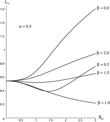
(a) $\alpha=0.5$

(b) $\alpha=2.0$

Figure 1: Dependence of the critical stretch $\lambda_{\text{cr}}<1$ for instability in compression for a magnetoelastic Mooney-Rivlin solid in plane strain on the non-dimensional measure $\bar{B}_{l2}$ of the magnetic field for several values of the magnetoelastic coupling parameters $\alpha$ and $\beta$.

Turning back to a phenomenological approach, we remark that the energy function (5.37) has quite good curve-fitting qualities for moderate fields. There are four parameters at hand, namely $\mu(0)$, $\alpha$, $\beta$, $\gamma$, two of which, $\mu(0)$ and $\beta$, may be determined from shear tests. Indeed Dorfmann and Ogden [24] show that in general the shear modulus for isotropic nonlinear magnetoelasticity is $2[\Omega_{1}+\Omega_{2}+I_{4}\Omega_{5}+I_{4}\Omega_{6}(3+2\kappa^{2})]$, where $\kappa$ is the amount of shear in a simple shear test. Here the modulus is independent of $\kappa$ and is given by

$$\mu(B_{l2})=\mu(0)+2\mu_{0}^{-1}\beta I_{4}.$$ (5.50)

This highlights the role of $\beta$ in increasing the mechanical stiffness of the material — through the shear modulus. Jolly et al. [9] conducted double lap shear tests on magneto-sensitive elastomers containing 10, 20, and 30% by volume of iron particles. From their Figure 7, we see that in the range $0\leq B_{l2}\leq 0.5$ Tesla, the variations of $\mu(B_{l2})$ resemble those of a parabolic profile such as the one suggested by (5.50). For the 10% iron by volume elastomer specimen, Table 1 in Jolly et al. [9] gives $\mu(0)=0.26$ MPa, and at $B_{l2}=0.5$ Tesla, we read off their Figure 7 that $\mu(0.5)-\mu(0)\simeq 0.07$ MPa, indicating that $\beta\simeq 0.18$. Similarly, for the 20% and the 30% iron by volume elastomer specimens we find $\beta\simeq 0.53$ and $\beta\simeq 0.72$, respectively.

Figure 2a (Figure 2b) illustrates the variation of the critical compression stretch with the amplitude of the dimensional magnetic induction vector, from 0 to 0.5 Tesla, for the 20% (30%) iron by volume elastomer, and for several values of $\alpha$. We remark than the presence of the magnetic field makes the two specimens slightly more stable than in the purely elastic case because all the critical compression stretch values are smaller than 0.5437. It is also clear that increasing the value of $\alpha$ makes the half-space more stable. However, it is worth noting that the 30% iron by volume specimen is slightly less stable than the 20% iron by volume specimen for the same values of $\alpha$.

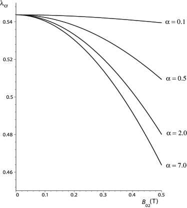
(a) $\beta=0.53$

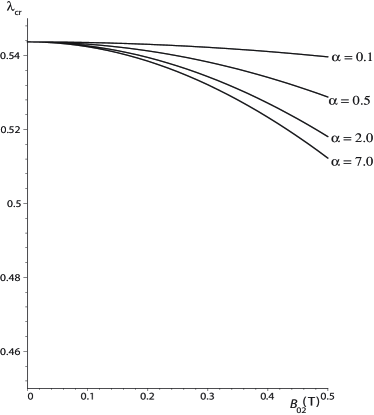
(b) $\beta=0.72$

Figure 2: Dependence of the critical stretch $\lambda_{\text{cr}}<1$ for instability in compression for a magnetoelastic Mooney-Rivlin solid in plane strain with the dimensional measure $B_{l2}$ of the magnetic field, for several values of the magnetoelastic coupling parameters $\alpha$ and $\beta$.

Appendix A Derivatives of the invariants with respect to $\boldsymbol{F}$ and $\boldsymbol{B}_{l}$

We derive the expressions for the first derivatives of the six invariants with respect to $\boldsymbol{F}$,

$$\dfrac{\partial I_{1}}{\partial F_{i\alpha}}=2F_{i\alpha},\qquad\dfrac{\partial I_{2}}{\partial F_{i\alpha}}=2(c_{\gamma\gamma}F_{i\alpha}-c_{\alpha\gamma}F_{i\gamma}),$$

$$\dfrac{\partial I_{3}}{\partial F_{i\alpha}}=2I_{3}F_{\alpha i}^{-1},\qquad\dfrac{\partial I_{4}}{\partial F_{i\alpha}}=0,\qquad\dfrac{\partial I_{5}}{\partial F_{i\alpha}}=2B_{l\alpha}(F_{i\gamma}B_{l\gamma}),$$

$$\dfrac{\partial I_{6}}{\partial F_{i\alpha}}=2(F_{i\gamma}B_{l\gamma}c_{\alpha\beta}B_{l\beta}+F_{i\gamma}c_{\gamma\beta}B_{l\beta}B_{l\alpha}),$$ (A.1)

and with respect to $\boldsymbol{B}_{l}$,

$$\dfrac{\partial I_{1}}{\partial B_{l\alpha}}=0, \dfrac{\partial I_{2}}{\partial B_{l\alpha}}=0, \dfrac{\partial I_{3}}{\partial B_{l\alpha}}=0,$$

$$\dfrac{\partial I_{4}}{\partial B_{l\alpha}}=2B_{l\alpha}, \dfrac{\partial I_{5}}{\partial B_{l\alpha}}=2c_{\alpha\beta}B_{l\beta}, \dfrac{\partial I_{6}}{\partial B_{l\alpha}}=2c_{\alpha\gamma}c_{\gamma\beta}B_{l\beta}.$$ (A.2)

The second derivatives of the invariants are computed as follows: first, the second derivatives with respect to $\boldsymbol{F}$,

$$\dfrac{\partial^{2}I_{1}}{\partial F_{i\alpha}\partial F_{j\beta}} =2\delta_{ij}\delta_{\alpha\beta},$$

$$\dfrac{\partial^{2}I_{2}}{\partial F_{i\alpha}\partial F_{j\beta}} =2(2F_{i\alpha}F_{j\beta}-F_{i\beta}F_{j\alpha}+c_{\gamma\gamma}\delta_{ij}\delta_{\alpha\beta}-b_{ij}\delta_{\alpha\beta}-c_{\alpha\beta}\delta_{ij}),$$

$$\dfrac{\partial^{2}I_{3}}{\partial F_{i\alpha}\partial F_{j\beta}} =4I_{3}F^{-1}_{\alpha i}F^{-1}_{\beta j}-2I_{3}F^{-1}_{\alpha j}F^{-1}_{\beta i},$$

$$\dfrac{\partial^{2}I_{4}}{\partial F_{i\alpha}\partial F_{j\beta}} =0,$$

$$\dfrac{\partial^{2}I_{5}}{\partial F_{i\alpha}\partial F_{j\beta}} =2\delta_{ij}B_{l\alpha}B_{l\beta},$$

$$\dfrac{\partial^{2}I_{6}}{\partial F_{i\alpha}\partial F_{j\beta}} =2[\delta_{ij}(c_{\alpha\gamma}B_{l\gamma}B_{l\beta}+c_{\beta\gamma}B_{l\gamma}B_{l\alpha})+\delta_{\alpha\beta}F_{i\gamma}B_{l\gamma}F_{j\delta}B_{l\delta}$$

$$\qquad\qquad\qquad+F_{i\gamma}B_{l\gamma}F_{j\alpha}B_{l\beta}+F_{j\gamma}B_{l\gamma}F_{i\beta}B_{l\alpha}+b_{ij}B_{l\alpha}B_{l\beta}];$$ (A.3)

next, the mixed derivatives with respect to $\boldsymbol{F}$ and $\boldsymbol{B}_{l}$,

$$\dfrac{\partial^{2}I_{1}}{\partial F_{i\alpha}\partial B_{l_{\beta}}}=0,\quad\dfrac{\partial^{2}I_{2}}{\partial F_{i\alpha}\partial B_{l_{\beta}}}=0,\quad\dfrac{\partial^{2}I_{3}}{\partial F_{i\alpha}\partial B_{l_{\beta}}}=0,\quad\dfrac{\partial^{2}I_{4}}{\partial F_{i\alpha}\partial B_{l_{\beta}}}=0,$$

$$\dfrac{\partial^{2}I_{5}}{\partial F_{i\alpha}\partial B_{l_{\beta}}}=2\delta_{\alpha\beta}F_{i\gamma}B_{l_{\gamma}}+2B_{l_{\alpha}}F_{i\beta},$$

$$\dfrac{\partial^{2}I_{6}}{\partial F_{i\alpha}\partial B_{l_{\beta}}}=2F_{i\beta}c_{\alpha\gamma}B_{l_{\gamma}}+2F_{i\gamma}B_{l_{\gamma}}c_{\alpha\beta}+2F_{i\gamma}c_{\gamma\beta}B_{l_{\alpha}}+2\delta_{\alpha\beta}F_{i\gamma}c_{\gamma\delta}B_{l\delta};$$ (A.4)

finally, the second derivatives with respect to $\boldsymbol{B}_{l}$,

$$\dfrac{\partial^{2}I_{1}}{\partial B_{l\alpha}\partial B_{l\beta}}=0, \dfrac{\partial^{2}I_{2}}{\partial B_{l\alpha}\partial B_{l\beta}}=0, \dfrac{\partial^{2}I_{3}}{\partial B_{l\alpha}\partial B_{l\beta}}=0,$$

$$\dfrac{\partial^{2}I_{4}}{\partial B_{l\alpha}\partial B_{l\beta}}=2\delta_{\alpha\beta}, \dfrac{\partial^{2}I_{5}}{\partial B_{l\alpha}\partial B_{l\beta}}=2c_{\alpha\beta}, \dfrac{\partial^{2}I_{6}}{\partial B_{l\alpha}\partial B_{l\beta}}=2c_{\alpha\gamma}c_{\gamma\beta}.$$ (A.5)

References

- [1] Bellan, C., Bossis, G.: Field dependence of viscoelastic properties of MR elastomers. Int. J. Mod. Phys. B 16, 2447–2453 (2002)
- [2] Rigbi, Z., Jilkén, L.: The response of an elastomer filled with soft ferrite to mechanical and magnetic influences. J. Magn. Magn. Mater. 37, 267–276 (1983)
- [3] Truesdell, C., Toupin, R.: The classical field theories. In: Handbuch der Physik, volume III/1. Springer, Berlin (1960)
- [4] Brown, W.F.: Magnetoelastic Interactions. Springer, Berlin (1966)
- [5] Yu, C.P., Tang, S.: Magneto-elastic waves in initially stressed conductors. ZAMP 17, 766–775 (1966)
- [6] Maugin, G.A.: Continuum Mechanics of Electromagnetic Solids. Series in Applied Mathematics and Mechanics, North-Holland, Amsterdam (1988)
- [7] Eringen, A.C., Maugin, G.A.: Electrodynamics of Continua. Springer, New York (1990)
- [8] Kovetz, A.: Electromagnetic Theory. University Press, Oxford (2000)
- [9] Jolly, M.R., Carlson, J.D., Munoz, B.C.: A model of the behaviour of magnetorheological materials. Smart Mater. Struct. 5, 607–614 (1996)
- [10] Dapino, M.J.: On magnetostrictive materials and their use in adaptive structures. Struct. Eng. Mech. 17, 303–329 (2004)
- [11] Dorfmann, A., Brigadnov, I.A.: Constitutive modelling of magneto-sensitive Cauchy-elastic solids. Comp. Mater. Sci. 29, 270–282 (2004)
- [12] Dorfmann, A., Ogden, R.W.: Nonlinear magnetoelastic deformations. Q. J. Mech. Appl. Math. 57, 599–622 (2004)
- [13] Kankanala, S.V., Triantafyllidis, N.: On finitely strained magnetorheological elastomers. J. Mech. Phys. Solids 52, 2869–2908 (2004)
- [14] McCarthy, M.F.: Wave propagation in nonlinear magneto-thermoelasticity. Proc. Vib. Prob. 8, 337–348 (1967)
- [15] van de Ven, A.A.F.: Interaction of Electromagnetic and Elastic Fields in Solid. PhD Thesis, Eindhoven University of Technology (1975)
- [16] Boulanger, Ph.: Influence d’un champ magnétique statique sur la réflexion d’une onde électromagnétique à la surface d’un conducteur parfait élastique. C.R. Acad. Sci. Paris Ser. A-B 285, B353–B356 (1977)
- [17] Boulanger, Ph.: Contribution à l’électrodynamique des continus élastiques et viscoélastiques. Acad. Roy. Belg. C1. Sci. Mem. Collect. 43, 4–47 (1978/79)
- [18] Maugin, G.A.: Wave motion in magnetizable deformable solids. Int. J. Eng. Sci. 19, 321–388 (1981)
- [19] Carroll, M.M., McCarthy, M.F.: Finite amplitude wave propagation in magnetized perfectly electrically conducting elastic materials. In: McCarthy, M.F., Hayes, M.A. (eds.) Elastic Wave Propagation, pp. 615–621. North-Holland, Amsterdam (1989)
- [20] Das, S.C., Acharya, D.P., Sengupta, P.R.: Magneto-visco-elastic surface waves in stressed conducting media. Sādh. 19, 337–346 (1994)
- [21] Spencer, A.J.M.: Theory of invariants. In: Eringen, A.C. (ed.) Continuum Physics, vol.1, pp. 239–353, Academic Press, New York (1971)
- [22] Dorfmann, A., Ogden, R.W.: Magnetoelastic modelling of elastomers. Eur. J. Mech. A. Solids 22, 497–507 (2003)
- [23] Dorfmann, A., Ogden, R.W.: Nonlinear magnetoelastic deformations of elastomers. Acta Mech. 167, 13–28 (2003)
- [24] Ogden, R.W., Dorfmann, A.: Magnetomechanical interactions in magneto-sensitive elastomers. In: Austrell and Kari (eds.) Constitutive Models for Rubber IV, pp. 531–556 (2005)
- [25] Bustamante, R., Ogden, R.W.: Transversely isotropic nonlinearly magnetoelastic solids. To appear (2007)
- [26] Pao, Y.H.: Electromagnetic forces in deformable continua. Mechanics Today 4, 209–306 (1978)
- [27] Steigmann, D.J.: Equilibrium theory for magnetic elastomers and magnetoelastic membranes. Int. J. Non-Linear Mech. 39, 1193–1216 (2004)
- [28] Ginder, J.M., Nichols, M.E., Ellie, L.D., Tardiff, J.L.: Magnetorheological elastomers: properties and applications. In: SPIE Conference on Smart Materials Technologies, pp. 131–138, California (1999)
- [29] Chadwick, P., Ogden, R.W.: On the definition of elastic moduli. Arch. Ration. Mech. Anal. 44, 41–53 (1971)
- [30] Chadwick, P.: The application of the Stroh formalism to prestressed elastic media. Math. Mech. Solids 2, 379–403 (1997)
- [31] Prikazchikov, D.A.: Surface and Edge Phenomena in Pre-Stressed Incompressible Elastic Solids. PhD thesis, University of Salford (2004)
- [32] Biot, M.A.: Mechanics of Incremental Deformations. John Wiley, New York (1965)
- [33] Ogden, R.W.: Elements of the theory of finite elasticity. In: Fu and Ogden (eds.) Nonlinear Elasticity: Theory and Applications, LMS lecture notes No. 283, pp.1–57. University Press, Cambridge (2001)
- [34] Destrade, M., Otténio, M., Pichugin, A.V., Rogerson, G.A.: Non-principal surface waves in deformed incompressible materials. Int. J. Eng. Sci. 42, 1092–1106 (2005)