The stress field in a pulled cork and
some subtle points in the
semi-inverse method of nonlinear elasticity

Abstract

In an attempt to describe cork-pulling, we model a cork as an incompressible rubber-like material and consider that it is subject to a helical shear deformation superimposed onto a shrink fit and a simple torsion. It turns out that this deformation field provides an insight into the possible appearance of secondary deformation fields for special classes of materials. We also find that these latent deformation fields are woken up by normal stress differences. We present some explicit examples based on the neo-Hookean, the generalized neo-Hookean, and the Mooney–Rivlin forms of the strain-energy density. Using the simple exact solution found in the neo-Hookean case, we conjecture that it is advantageous to accompany the usual vertical axial force by a twisting moment, in order to extrude a cork from the neck of a bottle efficiently. Then we analyse departures from the neo-Hookean behaviour by exact and by asymptotic analyses. In that process we are able to give an elegant and analytic example of secondary (or latent) deformations in the framework of nonlinear elasticity.

1 Introduction

Rubbers and elastomers are highly deformable solids which have the remarkable property of preserving their volume through any deformation. This permanent isochoricity can be incorporated into the equations of continuum mechanics through the concept of an internal constraint, here the constraint of incompressibility. Mathematically, the formulation of the constraint of incompressibility has led to the discovery of several exact solutions in isotropic finite elasticity, most notably to the controllable or universal solutions of Rivlin and co-workers (see for example Rivlin (1948)). Subsequently, Ericksen (1954) examined the problem of finding all such solutions. He found that there are no controllable finite deformations in isotropic compressible elasticity, except for homogeneous deformations (Ericksen 1955). The impact of that result on the theory of nonlinear elasticity was quite important and long-lasting, and for many years a palpable pessimism reigned about the possibility of finding exact solutions at all for compressible elastic materials. Then Currie & Hayes (1981) showed that one could obtain interesting classes of exact solutions, beyond the homogeneous universal deformations, if one restricted their attention to certain special classes of compressible materials. A string of results about the search for exact solutions in nonlinear elasticity followed. Now a long list exists of classes of exact solutions which are universal only relative to some special strain-energy functions (for a recent presentation of such classes see Fu and Ogden (2001).) These solutions can help us to understand the structure of the theory of nonlinear elasticity and to complement the celebrated solutions of Rivlin.

In the same vein, some recent efforts focused on determining the maximal strain energy for which a certain deformation field, fixed a priori, is admissible. This is a sort of inverse problem: find the elastic materials (that is, the functional form of the strain-energy function) for which a given deformation field is controllable (that is, for which the deformation is a solution to the equilibrium equations in the absence of body forces). A classical example illustrating such an approach is obtained by considering deformations of anti-plane shear type. Knowles (1977) shows that a non-trivial (non-homogeneous) equilibrium state of anti-plane shear is not always (universally) admissible, not only for compressible solids (as expected from Ericksen’s result) but also for incompressible solids (Horgan (1995) gives a survey of anti-plane shear deformations in nonlinear elasticity). Only for a special class of incompressible materials (inclusive of the so-called ‘generalized neo-Hookean materials’) is an anti-plane shear deformation controllable.

Let us consider for example the case of an elastic material filling the annular region between two coaxial cylinders, with the following boundary value problem: hold fixed the outer cylinder and pull the inner cylinder by applying a tension in the axial direction. It is well established that a solution to this problem, valid for every isotropic incompressible elastic solid, is obtained by assuming a priori that the deformation field is a pure axial shear. Now consider the corresponding problem for non-coaxial cylinders, thereby losing the axial symmetry. Then it is clear that we cannot expect the material to deform as prescribed by a pure axial shear deformation. Knowles’s result tells us that now the boundary value problem can be solved with a general anti-plane deformation (not axially symmetric) only for a subclass of incompressible isotropic elastic materials. Of course this restriction does not mean that for a generic material it is not possible to deform the annular material as prescribed by our boundary conditions, but rather that in general, these lead to a deformation field which is more complex than an anti-plane shear. And so, we expect secondary in-plane deformations.

The theory of non-Newtonian fluid dynamics has generated a substantial literature about secondary flows, see for example Fosdick & Serrin (1973). In solid mechanics it seems that only Fosdick & Kao (1978) and Mollica & Rajagopal (1997) produced some significant and beautiful examples of secondary deformations fields for the non-coaxial cylinders problem, although this topic is clearly of fundamental importance, not only from a theoretical point of view but also for technical applications.

In this paper we consider a complex deformation field in isotropic incompressible elasticity, to point out by an explicit example the situations just evoked and to elaborate on their possible impact on solid mechanics. Our deformation field takes advantage of the radial symmetry and therefore we find it convenient to visualize it by considering an elastic cylinder.

Let us imagine that a corkscrew has been driven through a cork (the cylinder) in a bottle. The inside of the bottleneck is the outer rigid cylinder and the idealization of the gallery carved out by the corkscrew constitutes the inner coaxial rigid cylinder. Our first deformation is purely radial, originated from the introduction of the cork into the bottleneck and then completed when the corkscrew penetrates the cork (a so-called shrink fit problem, which is a source of elastic residual stresses here). We call $A$, $B$ the respective inner and outer radii of the cork in the reference configuration and $r_{1}>A$, $r_{2}<B$ their current counterparts. Then we follow with a simple torsion combined to a helical shear, in order to model pulling the cork out of the bottleneck in the presence of a contact force. Figure 1 sketches this deformation.

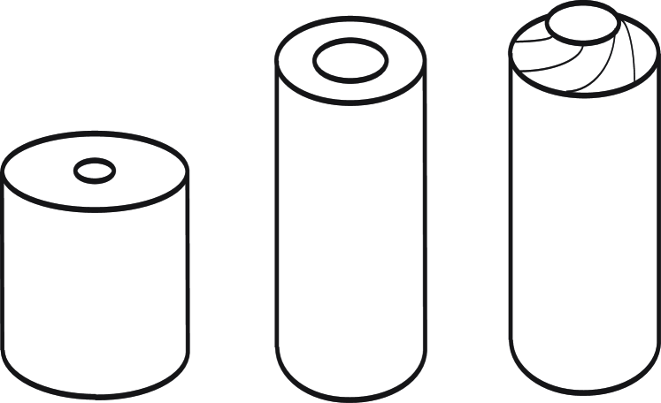
Figure 1: Shrink fit of an elastic tube, followed by the combination of simple torsion and helical shear. (The figure does not respect scales among the various deformations)

Of course we are aware of the shortcomings of our modelling with respect to the description of a ‘real’ cork-pulling problem, because no cork is an infinitely long cylinder, nor is a corkscrew perfectly straight. In addition, traditional corks made from bark are anisotropic (honeycomb mesoscopic structure) and possess the remarkable (and little-known) property of having an infinitesimal Poisson ratio equal to zero, see the review article by Gibson et al. (1981). However we note that polymer corks have appeared on the world wine market; they are made of elastomers, for which incompressible, isotropic elasticity seems like a reasonable framework (indeed the documentation of these synthetic wine stoppers indicates that they lengthen during the sealing process). We hope that this study provides a first step toward a nonlinear alternative to the linear elasticity testing protocols presented in the international standard ISO 9727. We also note that low-cost shock absorbers often consist of a moving metal cylinder, glued to the inner face of an elastomeric tube, whose outer face is glued to a fixed metal cylinder (Hill 1975).

The plan of the paper is the following. Section 2 is devoted to the derivation of the governing equations and to a detailed description of the boundary value problem. In §3 we specialize the analysis to the neo-Hookean strain-energy density, and find the corresponding exact solution. We use it to show that it is advantageous to add a twisting moment to an axial force when extruding a cork from a bottle. The neo-Hookean strain-energy density is linear with respect to the first principal invariant of the Cauchy-Green strain tensor. It is much used in Finite Elasticity theory, although it captures poorly the basic features of rubber behaviour (Saccomandi 2004). We thus investigate the consequence of departing from that strain-energy density. First, in §4 we consider the generalized neo-Hookean strain-energy density — non-linear with respect to the first principal invariant of the Cauchy-Green strain tensor — to show that in this case torsion is explicitly present in the solution for the axial shear displacement, but it is a second-order dependence. Next we consider in §5 the Mooney–Rivlin strain-energy density — linear with respect to the first and second principal invariants of the Cauchy-Green strain tensor — and find that it is then also possible to obtain an exact solution to our boundary value problem. Its expression is too cumbersome to manipulate and we resort to a small parameter asymptotic expansion from the neo-Hookean case. Section 6 concludes the paper with some remarks on the limitations of the semi-inverse method.

2 Basic equations

Consider a long hollow cylindrical tube, composed of an isotropic incompressible nonlinearly elastic material. At rest the tube is in the region

$$A\leq R\leq B,\qquad 0\leq\Theta\leq 2\pi,\qquad-\infty\leq Z\leq\infty,$$ (2.1)

where $(R,\Theta,Z)$ are the cylindrical coordinates associated with the undeformed configuration, and $A$ and $B$ are the inner and outer radii of the tube, respectively.

2.1 Equilibrium equations

Consider the general deformation obtained by the combination of radial dilatation, helical shear, and torsion, as

$$r=r(R),\qquad\theta=\Theta+g(R)+\tau Z,\qquad z=\lambda Z+w(R),$$ (2.2)

where $(r,\theta,z)$ are the cylindrical coordinates in the deformed configuration, $\tau$ is the amount of torsion and $\lambda$ is the stretch ratio in the $Z$ direction. Here, $g$ and $w$ are yet unknown functions of $R$ only (The classical case of pure torsion corresponds to $w=g=0$, see the textbooks by Ogden (1997) or by Atkin and Fox (2007), for instance.)

Hidden inside (2.2) is the shrink fit deformation

$$r=r(R),\qquad\theta=\Theta,\qquad z=\lambda Z,$$ (2.3)

which is (2.2) without any torsion nor helical shear ($\tau=g=w\equiv 0$).

The physical components of the deformation gradient $\boldsymbol{F}$ and of its inverse $\boldsymbol{F}^{-1}$ are then

$$\begin{bmatrix}r^{\prime}&0&0\\ rg^{\prime}&r/R&r\tau\\ w^{\prime}&0&\lambda\end{bmatrix},\qquad\begin{bmatrix}r\lambda/R&0&0\\ rw^{\prime}\tau-rg^{\prime}\lambda&r^{\prime}\lambda&-rr^{\prime}\tau\\ -rw^{\prime}/R&0&rr^{\prime}/R\end{bmatrix},$$ (2.4)

respectively. Note that we used the incompressibility constraint in order to compute $\boldsymbol{F}^{-1}$; it states that $\text{det }\boldsymbol{F}=1$, so that

$$r^{\prime}=\dfrac{R}{\lambda r}.$$ (2.5)

In our first deformation, the cylindrical tube is pressed into a cylindrical cavity with inner radius $r_{1}>A$ and outer radius $r_{2}<B$. It follows by integration of the equation above that

$$r(R)=\sqrt{\dfrac{R^{2}}{\lambda}+\alpha},$$ (2.6)

where now

$$\alpha=\frac{B^{2}r_{1}^{2}-A^{2}r_{2}^{2}}{B^{2}-A^{2}},\qquad\lambda=\frac{B^{2}-A^{2}}{r_{2}^{2}-r_{1}^{2}}.$$ (2.7)

We compute the physical components of the left Cauchy-Green strain tensor $\boldsymbol{B}\equiv\boldsymbol{FF}^{t}$ from (2.4) and find its first three principal invariants $I_{1}\equiv\text{tr }\boldsymbol{B}$, $I_{2}\equiv(\text{det }\boldsymbol{B})\text{tr }(\boldsymbol{B}^{-1})$, and $I_{3}\equiv\text{det }\boldsymbol{B}$ as

$$I_{1}=(r^{\prime})^{2}+(rg^{\prime})^{2}+(r/R)^{2}+(r\tau)^{2}+\lambda^{2}+(w^{\prime})^{2},$$

$$I_{2}=(r\lambda/R)^{2}+(rw^{\prime}\tau-rg^{\prime}\lambda)^{2}+(rw^{\prime}/R)^{2}+(R/r)^{2}+(1/\lambda)^{2}+(R\tau/\lambda)^{2},$$ (2.8)

and of course, $I_{3}=1$.

For a general incompressible hyperelastic solid, the Cauchy stress tensor $\boldsymbol{T}$ is related to the strain through

$$\boldsymbol{T}=-p\boldsymbol{I}+2W_{1}\boldsymbol{B}-2W_{2}\boldsymbol{B}^{-1},$$ (2.9)

where $p$ is the Lagrange multiplier introduced by the incompressibility constraint, $W=W(I_{1},I_{2})$ is the strain energy density, and $W_{i}\equiv\partial W/\partial I_{i}$. Having computed $\boldsymbol{B}^{-1}\equiv(\boldsymbol{F}^{t})^{-1}\boldsymbol{F}^{-1}$ from (2.4), we find that the components of $\boldsymbol{T}$ are

$$T_{rr}=-p+2W_{1}(r^{\prime})^{2}-2W_{2}\left[(r\lambda/R)^{2}+(rw^{\prime}\tau-rg^{\prime}\lambda)^{2}+(rw^{\prime}/R)^{2}\right],$$

$$T_{\theta\theta}=-p+2W_{1}\left[(rg^{\prime})^{2}+(r/R)^{2}+(r\tau)^{2}\right]-2W_{2}(R/r)^{2},$$

$$T_{zz}=-p+2W_{1}[\lambda^{2}+(w^{\prime})^{2}]-2W_{2}\left[(1/\lambda)^{2}+(R\tau/\lambda)^{2}\right],$$

$$T_{r\theta}=2W_{1}(rr^{\prime}g^{\prime})-2W_{2}(w^{\prime}\tau-g^{\prime}\lambda)R,$$

$$T_{rz}=2W_{1}(r^{\prime}w^{\prime})-2W_{2}\left[rRg^{\prime}\tau-rRw^{\prime}\tau^{2}/\lambda-rw^{\prime}/(\lambda R)\right],$$

$$T_{\theta z}=2W_{1}(rw^{\prime}g^{\prime}+r\lambda\tau)+2W_{2}(r^{\prime}R\tau).$$ (2.10)

Finally the equilibrium equations, in the absence of body forces, are: $\text{div }\boldsymbol{T}=\mathbf{0}$; for fields depending only on the radial coordinate as here, they reduce to

$$\dfrac{\text{d}T_{rr}}{\text{d}r}+\dfrac{T_{rr}-T_{\theta\theta}}{r}=0,\qquad\dfrac{\text{d}T_{r\theta}}{\text{d}r}+\frac{2}{r}T_{r\theta}=0,\qquad\dfrac{\text{d}T_{rz}}{\text{d}r}+\frac{1}{r}T_{rz}=0.$$ (2.11)

2.2 Boundary conditions

Now consider the inner face of the tube: we assume that it is subject to a vertical pull,

$$T_{rz}(A)=T_{0}^{A},\qquad T_{r\theta}(A)=0,$$ (2.12)

say. Then we can integrate the second and third equations of equilibrium (2.11)_2,3; we find that

$$T_{rz}(r)=\frac{r_{1}}{r}T_{0}^{A},\qquad T_{r\theta}(r)=0.$$ (2.13)

The outer face of the tube (in contact with the glass in the cork/bottle problem) remains fixed, so that

$$w(B)=0,\qquad g(B)=0,\qquad T_{rr}(B)=T_{0},$$ (2.14)

say. In addition to the axial traction applied on its inner face, the tube is subject to a resultant axial force $N$ (say) and a resultant moment $M$ (say),

$$N=\int_{0}^{2\pi}\int_{r_{1}}^{r_{2}}T_{zz}r\text{d}r\text{d}\theta,\qquad M=\int_{0}^{2\pi}\int_{r_{1}}^{r_{2}}T_{\theta z}r^{2}\text{d}r\text{d}\theta.$$ (2.15)

Note that the traction $T_{0}$ of (2.14) is not arbitrary but is instead determined by the shrink fit pre-deformation (2.3), by requiring that $N=0$ when $T_{0}^{A}=\tau=g=w\equiv 0$ (This process is detailed in the next section for the neo-Hookean material.) Therefore $T_{0}$ is connected with the stress field experienced by the cork when it is introduced in the bottleneck.

In the rest of the paper we aim at presenting results in dimensionless form. To this end we normalize the strain-energy density $W$ and the Cauchy stress tensor $\boldsymbol{T}$ with respect to $\mu$, the infinitesimal shear modulus; hence we introduce $\overline{W}$ and $\overline{\boldsymbol{T}}$ defined by

$$\overline{W}=\dfrac{W}{\mu},\qquad\overline{\boldsymbol{T}}=\dfrac{\boldsymbol{T}}{\mu}.$$ (2.16)

Similarly we introduce the following non-dimensional variables,

$$\eta=\dfrac{A}{B},\quad\overline{R}=\dfrac{R}{B},\quad\overline{r}_{i}=\dfrac{r_{i}}{B},\quad\overline{w}=\dfrac{w}{B},\quad\overline{\alpha}=\dfrac{\alpha}{B^{2}},\quad\overline{\tau}=B\tau,$$ (2.17)

so that $\eta\leq\overline{R}\leq 1$. Also, we find from (2.7) that

$$\overline{\alpha}=\dfrac{\overline{r}_{1}^{2}-\eta^{2}\overline{r}_{2}^{2}}{1-\eta^{2}},\qquad\lambda=\dfrac{1-\eta^{2}}{\overline{r}_{2}^{2}-\overline{r}_{1}^{2}}.$$ (2.18)

Turning to our cork or shock absorber problems, we imagine that the inner metal cylinder is introduced into a pre-existing cylindrical cavity (this precaution ensures a one-to-one correspondence of the material points between the reference and the current configurations). In our upcoming numerical simulations, we take $A=B/10$ so that $\eta=0.1$; we consider that the outer radius is shrunk by 10%: $r_{2}=0.9B$, and that the inner radius has doubled: $r_{1}=2A$; finally we apply a traction whose magnitude is half the infinitesimal shear modulus: $|T_{0}^{A}|=\mu/2$. This gives

$$\overline{\alpha}\simeq 3.22\times 10^{-2},\qquad\lambda\simeq 1.286,\qquad\overline{T}_{0}^{A}=-0.5.$$ (2.19)

At this point it is possible to state clearly our main observation. A first glance at the boundary conditions, in particular at the requirements that $g$ be zero on the outer face of the tube, gives the expectation that $g\equiv 0$ everywhere is a solution to our boundary value problem, at least for some simple forms of the constitutive equations. In what follows we find that for the so-called ‘neo-Hookean’ solids, $g\equiv 0$ is indeed a solution, whether there is a torsion $\tau$ or not. However if the solid is not neo-Hookean, then it is necessary that $g\neq 0$ when $\tau\neq 0$, and the picture becomes more complex. For this reason, we classify as ‘purely academic’ the question: which is the most general strain-energy density for which it is possible to solve the above boundary value problem with $g\equiv 0$ ? Indeed there is no ‘real world’ material whose behaviour is ever going to be described exactly by that strain-energy density (supposing it exists). Instead a more pertinent issue to raise for ‘real word applications’ is whether we are able to evaluate the importance of latent (secondary) stress fields, because they are bound to be woken up (triggered) by the deformation.

3 neo-Hookean materials

First we consider the special strain energy density which generates the class of neo-Hookean materials, namely

$$W=(I_{1}-3)/2,\qquad\text{so that}\qquad 2W_{1}=1,\qquad W_{2}=0.$$ (3.1)

Note that here and hereafter, we use the non-dimensional quantities introduced previously, from which we drop the overbar for convenience. Hence the components of the (non-dimensional) stress field in a neo-Hookean material reduce to

$$T_{rr}=-p+(r^{\prime})^{2}, T_{\theta\theta}=-p+(rg^{\prime})^{2}+(r/R)^{2}+(r\tau)^{2},$$

$$T_{zz}=-p+\lambda^{2}+(w^{\prime})^{2}, T_{r\theta}=rr^{\prime}g^{\prime},$$

$$T_{rz}=r^{\prime}w^{\prime}, T_{\theta z}=rg^{\prime}w^{\prime}+r\lambda\tau.$$ (3.2)

Substituting into (2.13) we find that

$$w^{\prime}=\lambda r_{1}T_{0}^{A}/R,\qquad g^{\prime}=0,$$ (3.3)

and by integration, using (2.14), that

$$w=\lambda r_{1}T_{0}^{A}\ln R,\qquad g=0.$$ (3.4)

In Figure 2a, we present a rectangle in the tube at rest. It is delimited by $0.1\leq R\leq 1.0$ and $0.0\leq Z\leq 1.0$. Then it is subject to the deformation corresponding to the numerical values of (2.19). To generate Figure 2b, we computed the resulting shape for a neo-Hookean tube, using (2.2), (2.6), and (3.4).

 

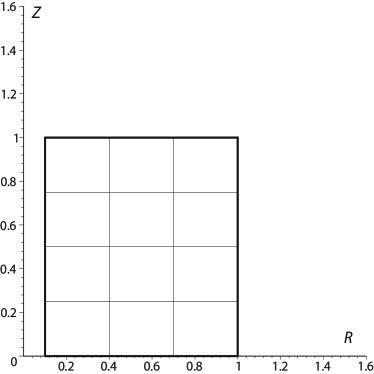
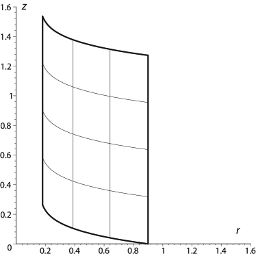
Figure 2: Pulling on the inside face of a neo-Hookean tube. Here the vertical axis is the symmetry axis of the tube.

Now that we know the ful deformation field, see (2.2) and (3.4), we can compute $T_{rr}-T_{\theta\theta}$ from (3.2) and deduce $T_{rr}$ by integration of (2.11)₁, with initial condition (2.14)₃. Then the other field quantities follow from the rest of (3.2). In the end we find in turn that

$$T_{rr}=\frac{1}{2\lambda}\left\{\ln\frac{\lambda r_{2}^{2}R^{2}}{R^{2}+\alpha\lambda}+(R^{2}-1)\left[\frac{\alpha}{r_{2}^{2}\left(R^{2}+\alpha\lambda\right)}+\tau^{2}\right]\right\}+T_{0},$$

$$T_{\theta\theta}=T_{rr}+\left(\frac{R^{2}}{\lambda}+\alpha\right)\left(\frac{1}{R^{2}}+\tau^{2}\right)-\frac{R^{2}}{\lambda(R^{2}+\alpha\lambda)},$$

$$T_{zz}=T_{rr}+\lambda^{2}\left(1+\frac{r_{1}^{2}(T_{0}^{A})^{2}}{R^{2}}\right)-\frac{R^{2}}{\lambda(R^{2}+\alpha\lambda)},$$ (3.5)

(where we used the identity $1+\alpha\lambda=\lambda r_{2}^{2}$, see (2.6) with $R=1$), and that

$$T_{r\theta}=0,\qquad T_{rz}=\dfrac{r_{1}}{\sqrt{\dfrac{R^{2}}{\lambda}+\alpha}}T_{0}^{A},\qquad T_{\theta z}=\lambda\tau\sqrt{\dfrac{R^{2}}{\lambda}+\alpha}.$$ (3.6)

The constant $T_{0}$ is fixed by the shrink fit pre-deformation (2.3), imposing that $N=0$ when $\tau=g=w=T_{0}^{A}\equiv 0$, or

$$(T_{0}+\lambda^{2})(1-\eta^{2})+\frac{1}{\lambda}\int_{\eta}^{1}\left[\ln\frac{\lambda r_{2}^{2}R^{2}}{R^{2}+\alpha\lambda}+\frac{\alpha(R^{2}-1)}{r_{2}^{2}(R^{2}+\alpha\lambda)}-\frac{2R^{2}}{R^{2}+\alpha\lambda}\right]R\text{d}R=0.$$ (3.7)

Using this, and (2.15), (3.5), (3.6), we find the following expressions for the resultant moment,

$$M=\pi(r_{2}^{4}-r_{1}^{4})\lambda\tau/2,$$ (3.8)

and for the axial force,

$$N=2\pi\lambda r_{1}^{2}|\ln\eta|\left(T_{0}^{A}\right)^{2}-\frac{\pi}{4}(r_{2}^{2}-r_{1}^{2})^{2}\tau^{2}.$$ (3.9)

We now have a clear picture of the response of a neo-Hookean solid to the deformation (2.2), with the boundary conditions of §2$\,b$. First we saw that here the contribution $g(R)$ is not required for the azimuthal displacement, whether there is a torsion $\tau$ or not. Also, if a moment $M\neq 0$ is applied, then the tube suffers an amount of torsion $\tau\neq 0$ proportional to $M$. On the other hand, if the tube is pulled by the application of an axial force only ($N\neq 0$) and no moment ($M=0$), then $\tau=0$ and no azimuthal shear occurs at all.

When we try to apply our results to the extrusion of a cork from the neck of a bottle, the following remarks seem to be relevant. From the elementary theory of Coulomb friction, it is known that the pulled cork starts to move when, in modulus, the friction force exerted on the neck surface is equal to the normal force times the coefficient of static friction. In our case this means that

$$\sqrt{\left|T_{rz}(1)\right|^{2}+\left|T_{r\theta}(1)\right|^{2}}=f_{S}\left|T_{rr}(1)\right|=f_{S}\left|T_{0}\right|,$$ (3.10)

where $f_{S}$ is the coefficient of static friction. Using (2.12) and (2.13), we find that the elements of the left handside of this inequality are

$$T_{rz}(1)=(r_{1}/r_{2})T_{0}^{A},\qquad T_{r\theta}(1)=0.$$ (3.11)

Now, our main concern is to understand if it is better to apply a moment $M\neq 0$ when uncorking a bottle, than to pull only. To address this question we note that the left handside of inequality (3.10) increases when $|T_{0}^{A}|$ increases; on the other hand, combining (3.8) and (3.9), we have

$$(T_{0}^{A})^{2}=\left[N+\frac{1}{\pi\lambda^{2}(r_{1}^{2}+r_{2}^{2})^{2}}M^{2}\right]/(2\pi\lambda r_{1}^{2}|\ln\eta|),$$ (3.12)

It is now clear, that for a fixed value of $T_{0}^{A}$, in the case $M\neq 0$, it is necessary to apply an axial force whose intensity is less than the one in the case $M=0$. Moreover, the equation above shows that $\left(T_{0}^{A}\right)^{2}$ grows linearly with $N$ but quadratically with $M$. With respect to efficient cork-pulling, the conclusion is that adding a twisting moment to a given pure axial force is more advantageous than solely increasing the vertical pull. Moreover, we observe that a moment is applied by using a lever and this is always more convenient from an energetic point of view.

Recall that we made several simplifying assumptions to reach these results: not only infinite axial length, incompressibility, and isotropy, but also the choice of a truly special strain energy density. In the next two sections we depart from the neo-Hookean model.

4 Generalized neo-Hookean materials

As a first broadening of the neo-Hookean strain-energy density (3.1), we consider generalized neo-Hookean materials, for which the strain-energy density is a nonlinear function of the first invariant $I_{1}$ only,

$$W=\widehat{W}(I_{1}),$$ (4.1)

say. To gain access to the Cauchy stress components in this context, it suffices to take $W_{2}=0$ and $W_{1}=\widehat{W}^{\prime}$ in equations (2.1). In particular, $T_{r\theta}=2rr^{\prime}g^{\prime}\widehat{W}^{\prime}$, and the integrated equation of equilibrium (2.13)₂ gives $g^{\prime}=0$. Integrating, with (2.12) as an initial value, we find that

$$g\equiv 0.$$ (4.2)

Hence, just as in the neo-Hookean case, azimuthal shear can be avoided altogether, whether there is a torsion $\tau$ or not. We are left with an equation for the axial shear, namely (2.13)₁, which here reads

$$2\widehat{W}^{\prime}(I_{1})w^{\prime}(R)=\frac{\lambda r_{1}}{R}T_{0}^{A}.$$ (4.3)

Obviously the same steps as those taken for neo-Hookean solids may be followed here for any given strain energy density (4.1), but now by resorting to a numerical treatment. Horgan & Saccomandi (2003$a$) show, through some specific examples of hardening generalized neo-Hookean solids, how rapidly involved the analysis becomes, even when there is only helical shear and no shrink fit.

Instead we simply point out some striking differences between our present situation and the neo-Hookean case. We remark that $I_{1}$ is of the form (2.1)₁ at $g\equiv 0$ that is,

$$I_{1}=\lambda^{2}+\frac{R^{2}}{\lambda(R^{2}+\alpha\lambda)}+\left(\frac{R^{2}}{\lambda}+\alpha\right)\left(\frac{1}{R^{2}}+\tau^{2}\right)+[w^{\prime}(R)]^{2}.$$ (4.4)

It follows that (4.3) is a nonlinear differential equation for $w^{\prime}$, in contrast with the neo-Hookean case. Another contrast is that the axial shear $w$ is now intimately coupled to the torsion parameter $\tau$, and that this dependence is a second-order effect ($\tau$ appears above as $\tau^{2}$).

A similar problem where the azimuthal shear has not been ignored, but the axial shear has been considered null i.e. $w\equiv 0$ has been recently considered by Wineman (2005).

5 Mooney–Rivlin materials

In this section we specialize the general equations of §2 to the Mooney–Rivlin form of the strain-energy density, which in its non-dimensional form reads

$$W=\frac{I_{1}-3+m(I_{2}-3)}{2(1+m)},\quad\text{so that}\quad 2W_{1}=\frac{1}{1+m}\quad 2W_{2}=\frac{m}{1+m},$$ (5.1)

where $m>0$ is a material parameter, distinguishing the Mooney–Rivlin material from the neo-Hookean material (3.1), and also allowing a dependence on the second principal strain invariant $I_{2}$, in contrast to the generalized neo-Hookean solids of the previous section.

Then the integrated equations of equilibrium (2.13) read

$$\left(R+m\tau^{2}r^{2}R+mr^{2}/R\right)w^{\prime}-(m\tau\lambda r^{2}R)g^{\prime}=(1+m)\lambda r_{1}T_{0}^{A},$$

$$(m\tau\lambda)w^{\prime}-(1+m\lambda^{2})g^{\prime}=0.$$ (5.2)

First we ask ourselves if it is possible to avoid torsion during the pulling of the inner face. Taking $\tau=0$ above gives

$$(R+mr^{2}/R)w^{\prime}=(1+m)\lambda r_{1}T_{0}^{A},\qquad g^{\prime}=0.$$ (5.3)

It follows that here it is indeed possible to solve our boundary value problem. We find

$$w=\lambda r_{1}T_{0}^{A}\ \dfrac{\lambda(1+m)}{2(\lambda+m)}\ln\left[\frac{m\alpha\lambda+(\lambda+m)R^{2}}{m\alpha\lambda+(\lambda+m)}\right],\qquad g=0.$$ (5.4)

However if $\tau\neq 0$, then it is necessary that $g\neq 0$, otherwise (5.2)₂ gives $w^{\prime}=0$ while (5.2)₁ gives $w^{\prime}\neq 0$, a contradiction. This constitutes the first departure from the neo-Hookean and generalized neo-Hookean behaviours: torsion ($\tau\neq 0$) is necessarily accompanied by azimuthal shear ($g\neq 0$).

In the case $\tau\neq 0$, we introduce the function $\Lambda=\Lambda(R)$ defined as

$$\Lambda(R)=(R+mr^{2}/R)(1+m\lambda^{2})+m\tau^{2}r^{2}R,$$ (5.5)

(recall that $r=r(R)$ is given explicitly in (2.6).) We then solve the system (5.2) for $w^{\prime}$ and $g^{\prime}$ as

$$w^{\prime}=(1+m)(1+m\lambda^{2})\lambda\dfrac{T_{0}^{A}}{\Lambda(R)}r_{1},\qquad g^{\prime}=m(1+m)\lambda^{2}\dfrac{T_{0}^{A}}{\Lambda(R)}\tau r_{1},$$ (5.6)

making clear the link between $g$ and $\tau$. Thus for the Mooney–Rivlin material, the azimuthal shear $g$ is a latent mode of deformation; it is woken up by any amount of torsion $\tau$. Recall that at first sight, the azimuthal shear component of the deformation (2.2) seemed inessential to satisfy the boundary conditions, especially in view of the boundary condition $g(1)=0$. However, a non-zero $W_{2}$ term in the constitutive equation clearly couples the effects of a torsion and of an azimuthal shear, as displayed explicitly by the presence of $\tau$ in the expression for $g^{\prime}$ above.

It is perfectly possible to integrate equations (5.6) in the general case, but to save space we do not reproduce the resulting long expressions. With them, we generated the deformation field picture of Figure 3a and Figure 3b. There we took the numerical values of (2.19) for $\alpha$, $\lambda$, $T_{0}^{A}$; we took a Mooney–Rivlin solid with $m=5.0$; we imposed a torsion of amount $\tau=0.5$; and we looked at the deformation field in the plane $Z=1$ (reference configuration) and $z=\lambda$ (current configuration).

 

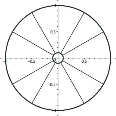
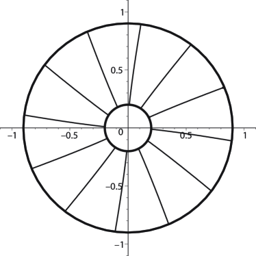
Figure 3: Pulling on the inside face of a Mooney–Rivlin tube, with a clockwise torsion.

Although the secondary fields appear to be slight in the picture, they are nonetheless truly present and cannot be neglected. To show this we consider a perturbation method to obtain simpler solutions and to understand the effect of the coupling, by taking $m$ small. Then integrating (5.6), we find at first order that

$$\dfrac{w}{r_{1}T_{0}^{A}}\simeq(1+m)\lambda\ln{R}-\dfrac{1}{2}m\left[\tau^{2}R^{2}+2(1+\tau^{2}\alpha\lambda)\ln R-\alpha\lambda/R^{2}-\tau^{2}+\alpha\lambda\right],$$

$$\dfrac{g}{r_{1}T_{0}^{A}}\simeq\lambda^{2}\tau m\ln{R}.$$ (5.7)

Hence, the secondary field $g$ exists even for a nearly neo-Hookean solid (if $m$ is small, then $g$ of order $m$.) Interestingly we also note that the azimuthal shear $g$ in (5) varies in a homogeneous and linear manner with respect to the torsion parameter $\tau$ and in a quadratic manner with respect to the axial stretch $\lambda$, showing that that the presence of this secondary deformation field cannot be neglected when the effects of the prestress and of the torsion are both taken into account. To complete the picture, we use the first-order approximations

$$2W_{1}\simeq 1-m,\qquad 2W_{2}\simeq m,$$ (5.8)

to obtain the stress field as

$$T_{rr}\simeq-p+\left(1-m\right)(r^{\prime})^{2}-m\left\{(r\lambda/R)^{2}+\left[(r\tau)^{2}+(r/R)^{2}\right]\left(\lambda r_{1}T_{0}^{A}\right)^{2}/R^{2}\right\},$$

$$T_{\theta\theta}\simeq-p+\left(1-m\right)\left[(r/R)^{2}+(r\tau)^{2}\right]-m(R/r)^{2},$$

$$T_{zz}\simeq-p+\left(\lambda T_{0}^{A}r_{1}\right)^{2}\left[\left(1+2m\lambda^{2}\right)\frac{1}{R^{2}}-\frac{2}{R}\left(\frac{\tau^{2}r^{2}}{R}+\frac{r^{2}}{R^{3}}+\frac{\lambda^{2}}{R}-\frac{1}{2R}\right)m\right]$$

$$\hskip 57.47469pt+\left(1-m\right)\lambda^{2}-m\left[(1/\lambda)^{2}+(R\tau/\lambda)^{2}\right],$$

$$T_{r\theta}\simeq rr^{\prime}g^{\prime}-m\lambda r_{1}T_{0}^{A}\tau,$$

$$T_{rz}\simeq\left(1-m\right)(r^{\prime}w^{\prime})+m\lambda r_{1}T_{0}^{A}\left[rR\tau^{2}/\lambda+r/(\lambda R)\right]/R,$$

$$T_{\theta z}\simeq\left(1-m\right)r\lambda\tau+\lambda rr_{1}T_{0}^{A}g^{\prime}/R+m(r^{\prime}R\tau).$$ (5.9)

Using this stress field it is straightforward, but long and cumbersome, to derive the analogue for a Mooney–Rivlin solid with a small $m$ of relation (3.12) (which was established for neo-Hookean solids.) However nothing truly new is gained from these complex formulas with respect to the simple neo-Hookean case, and we do not pursue this aspect any further.

6 Conclusion

In non-Newtonian fluid mechanics and in turbulence theory, the existence of shear-induced normal stresses on planes transverse to the direction of shear is at the root of some important phenomena occurring in the flow of fluid down pipes of non-circular cross section (Fosdick & Serrin 1973). In other words, pure parallel flows in tubes without axial symmetry are possible only when we consider the classical theory of Navier-Stokes equations or the linear theory of turbulence or tubes of circular cross section.

In nonlinear elasticity theory, similar phenomena are reported. Hence Fosdick & Kao (1978) and Mollica & Rajagopal (1997) show that for general isotropic incompressible materials, an anti-plane shear deformation of a cylinder with non axial-symmetric cross section causes a secondary in-plane deformation field, because of normal stress differences. Horgan & Saccomandi (2003$b$) give a detailed discussion of how the anti-plane shear deformation field couples with the in-plane deformation field in a generalized neo-Hookean solid.

The appearance of what we called here latent deformations is quite general and common. For example it is known in compressible nonlinear elasticity that pure torsion is possible only in a special class of materials, but we know that torsion plus a radial displacement is possible in all compressible isotropic elastic materials (Polignone & Horgan 1991) (Here we signal that ‘possible in all materials’ is not equivalent to ‘universal’, because the corresponding radial deformation differs from one material to another.)

In this paper we give an example where axial symmetry holds, where the boundary conditions suggest that an axial shear deformation field is sufficient to solve the boundary value problem, and where nevertheless, the normal stress difference wakes up a latent azimuthal shear deformation. Moreover, because we are able to find some explicit exact solutions by some perturbation techniques, we are able to evaluate the importance of the latent deformation. Indeed, we show that if a certain constitutive parameter $m$ (distinguishing a neo-Hookean solid from a Mooney–Rivlin solid) is zero or if the torsion parameter $\tau$ is zero, then the solution to the boundary value problem can be found only in terms of the axial shear deformation field; if these two parameters are not zero — even if they are small — then the latent mode of deformation is quantitatively appreciable.

In conclusion we suggest that it is not crucial to determine the class of materials for which a given deformation field is possible. Rather it is crucial to classify all the latent deformations associated with a given deformation field in such a way that this field is controllable for the entire class of materials. Indeed, no real material, even when we accept that its mechanical behaviour is purely elastic, is ever going to be described exactly by a special choice of strain-energy. Looking for special classes of materials for which special deformations fields are admissible may mislead us in our understanding of the nonlinear mechanical behaviour of materials.

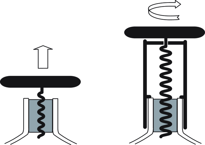
Figure 4: There are two main types of corkscrews: one that relies on pulling only (left) and one that adds a twist to the cork-pulling action (right). The analysis developed in this paper indicates that the second type is more efficient.

To finish the paper on a light note, we evoke a classic wine party dilemma: which kind of corkscrew system requires the least effort to uncork a bottle? Figure 4 sketches the two working principles commonly found in commercial corkscrews. The most common (on the left) relies on pulling only (directly or through levers) and the other type (on the right) relies on a combination of pulling and twisting. Notwithstanding the shortcomings of this paper’s modelling with respect to an actual uncorking, the authors are confident that they have provided a scientific argument to those wine amateurs who favour the second type of corkscrews over the first.