Interface Waves
in Pre-Stressed Incompressible Solids

Abstract

We study incremental wave propagation for what is seemingly the simplest boundary value problem, namely that constitued by the plane interface of a semi-infinite solid. With a view to model loaded elastomers and soft tissues, we focus on incompressible solids, subjected to large homogeneous static deformations. The resulting strain-induced anisotropy complicates matters for the incremental boundary value problem, but we transpose and take advantage of powerful techniques and results from the linear anisotropic elastodynamics theory. In particular we cover several situations where fully explicit secular equations can be derived, including Rayleigh and Stoneley waves in principal directions, and Rayleigh waves polarized in a principal plane or propagating in any direction in a principal plane. We also discuss the merits of polynomial secular equations with respect to more robust, but less transparent, exact secular equations.

Chapter 1 Introduction

The term “acousto-elastic effect” describes the interplay between the static deformation of an elastic solid and the motion of an elastic wave. If both the deformation and the motion are of infinitesimal amplitude, then all the governing equations are linearized, see for instance the Chapter by Norris for examples and applications or the experimental results of Pao et al. (1984). If both the deformation and the motion are of finite amplitude, then the resulting governing equations are highly nonlinear, and their resolution is the subject of much research, see the Chapter by Fu for the weakly nonlinear theory and the Chapter by Saccomandi for the fully nonlinear theory.

In between those two situations lies the theory of “small-on-large”, also known as the theory of “incremental” motions, where the wave is an infinitesimal perturbation superimposed onto the large static homogeneous deformation of a generic hyperelastic solid. There, the homogeneous character of the static deformation and the linear character of the incremental equations of motion ensure that the calculations are valid for any strain energy density (to be specified later for applications, if necessary). The next Section of this Chapter briefly recalls the governing equations of incremental motions (see the Chapter by Ogden for their derivation).

It turns out that many similarities can be drawn between the equations of incremental motions and those of linear anisotropic elasticity, with the main difference that in the latter case, the anisotropy is set once and for all for a given crystal whereas in the former case, it is strain-induced and susceptible to great variations from one configuration to another. Using the similarities, we may transpose the so-called Stroh formulation and exploit its many results; on the other hand, when focussing on the differences, we may highlight the influences of the pre-stress and of the choice of a strain-energy density on the propagation of waves. In this Chapter, attention is restricted to waves at the interface of pre-deformed, semi-infinite solids, in contact either with vacuum (Rayleigh waves) or with another solid (Stoneley waves). With a view to model elastomers and biological soft tissues, the solids are considered to be incompressible (mathematically, this internal constraint lightens somewhat the expressions but does not prove essential to the resolution).

Several situations are treated: principal wave propagation in Section 3, principal polarization in Section 4, and principal plane propagation in Section 5. The emphasis is on deriving explicit secular equations in polynomial form, using some simple “fundamental equations” derived at the end of Section 2. Of course, as the setting gets more and more involved, so does the search for a polynomial secular equation; eventually its degree becomes too high for comfort and other techniques are required. The concluding section (Section 6) discusses the pros and cons of such equations, as opposed to exact, non-explicit, secular equations, free of spurious roots.

Chapter 2 Basic equations

1 Finite deformation

Consider an isotropic, incompressible, hyperelastic solid at rest, characterized by a mass density $\rho$ and a strain energy function $W$. Then subject it to a large, static, homogeneous deformation (“the pre-strain”) carrying the particle at $\boldsymbol{X}$ in the undeformed configuration to the position $\boldsymbol{x}$ in the deformed configuration.

Call $\boldsymbol{F}=\partial\boldsymbol{x}/\partial\boldsymbol{X}$ the corresponding constant deformation gradient and $\boldsymbol{B}=\boldsymbol{FF}^{t}$ the associated left Cauchy-Green strain tensor. This tensor being symmetric, the directions of its eigenvectors are orthogonal; they are called the principal axes of pre-strain or in short, the principal axes. Also, the eigenvalues of $\boldsymbol{B}$ are positive, $\lambda_{1}^{2}$, $\lambda_{2}^{2}$, $\lambda_{3}^{2}$, say, and $\lambda_{1}$, $\lambda_{2}$, $\lambda_{3}$ are called the principal stretches. Figure 1 shows how a unit cube with edges aligned with the principal axes, is transformed by the pre-strain.

Figure 1: Finite homogeneous deformation of a unit cube.

Note that because the solid is incompressible, its volume is preserved through any deformation so that here,

$$\lambda_{1}\lambda_{2}\lambda_{3}=1.$$ (1)

The first two principal invariants of strain are defined as

$$I_{1}=\text{tr }\boldsymbol{B},\quad I_{2}=[(\text{tr }\boldsymbol{B})^{2}-\text{tr }(\boldsymbol{B}^{2})]/2.$$ (2)

In the Cartesian coordinate system aligned with the principal axes, $\boldsymbol{B}$ is diagonal. Calling $\boldsymbol{e}_{1}$, $\boldsymbol{e}_{2}$, $\boldsymbol{e}_{3}$, the unit vectors in the $x_{1}$, $x_{2}$, $x_{3}$ directions, respectively, we have

$$\boldsymbol{B}=\lambda_{1}^{2}\boldsymbol{e}_{1}\otimes\boldsymbol{e}_{1}+\lambda_{2}^{2}\boldsymbol{e}_{2}\otimes\boldsymbol{e}_{2}+\lambda_{3}^{2}\boldsymbol{e}_{3}\otimes\boldsymbol{e}_{3},$$ (3)

and the computation of $I_{1}$, $I_{2}$ there gives

$$I_{1}=\lambda_{1}^{2}+\lambda_{2}^{2}+\lambda_{3}^{2},\quad I_{2}=\lambda_{1}^{2}\lambda_{2}^{2}+\lambda_{2}^{2}\lambda_{3}^{2}+\lambda_{3}^{2}\lambda_{1}^{2}.$$ (4)

For an isotropic solid, $W$ may be given as a function of the invariants: $W=W(I_{1},I_{2})$ or equivalently, as a symmetric function of the principal stretches: $W=W(\lambda_{1},\lambda_{2},\lambda_{3})$, according to what is most convenient for the analysis or according to how $W$ has been determined experimentally. With the first choice, the constant Cauchy stress (“the pre-stress”) necessary to maintain the solid in its state of finite homogeneous deformation is

$$\boldsymbol{\sigma}=-p\boldsymbol{I}+2(\partial W/\partial I_{1}+I_{1}\partial W/\partial I_{2})\boldsymbol{B}-2(\partial W/\partial I_{2})\boldsymbol{B}^{2},$$ (5)

where $p$ is a Lagrange multiplier due to the constraint of incompressibility (a yet arbitrary constant scalar to be determined from initial and boundary conditions.) With the second choice, the non-zero components of $\boldsymbol{\sigma}$ relative to the principal axes are written as

$$\sigma_{i}=-p+\lambda_{i}\partial W/\partial\lambda_{i},\qquad i=1,2,3\text{ (no sum)}.$$ (6)

The proof for the equivalence between (5) and (6) relies on the connections (4).

2 Incremental equations

Consider a half-space filled with an incompressible hyperelastic solid subject to a large homogeneous deformation. We take the Cartesian coordinate system ($\hat{x}_{1}$, $\hat{x}_{2}$, $\hat{x}_{3}$) to be oriented so that the boundary is at $\hat{x}_{2}=0$, and we study the propagation in the $\hat{x}_{1}$ direction of an infinitesimal interface wave in the solid.

This wave is inhomogeneous as it progresses in an harmonic manner in a direction lying in the interface, while its amplitude decays with distance from the boundary.

We call $\boldsymbol{u}$ the mechanical displacement associated with the wave, and $\dot{p}$ the increment in the Lagrange multiplier $p$ due to incompressibility. The incremental nominal stress tensor $\boldsymbol{s}$ has components

$$s_{ji}=\mathcal{A}_{0jilk}u_{k,l}+pu_{j,i}-\dot{p}\delta_{ij},$$ (7)

where the comma denotes partial differentiation with respect to the coordinates $\hat{x}_{1}$, $\hat{x}_{2}$, $\hat{x}_{3}$. Here, $\boldsymbol{\mathcal{A}_{0}}$ is the fourth-order tensor of instantaneous elastic moduli, with components

$$\mathcal{A}_{0jilk}=F_{j\alpha}F_{l\beta}\dfrac{\partial^{2}W}{F_{i\alpha}F_{k\beta}}=\mathcal{A}_{0lkji}.$$ (8)

Note that due to the symmetry above, $\boldsymbol{\mathcal{A}_{0}}$ has in general 45 independent components. In the principal axes coordinate system ($x_{1}x_{2}x_{3}$) however, there are only 15 independent non-zero components; they are (Ogden, 2001):

$$\mathcal{A}_{0iijj}=\lambda_{i}\lambda_{j}W_{ij},$$

$$\mathcal{A}_{0ijij}=(\lambda_{i}W_{i}-\lambda_{j}W_{j})\lambda_{i}^{2}/(\lambda_{i}^{2}-\lambda_{j}^{2}), i\neq j,\quad\lambda_{i}\neq\lambda_{j},$$

$$\mathcal{A}_{0ijij}=(\mathcal{A}_{0iiii}-\mathcal{A}_{0iijj}+\lambda_{i}W_{i})/2, i\neq j,\quad\lambda_{i}=\lambda_{j},$$

$$\mathcal{A}_{0ijji}=\mathcal{A}_{0jiij}=\mathcal{A}_{0ijij}-\lambda_{i}W_{i}, i\neq j,$$ (9)

(no sums on repeated indexes here), where $W_{j}=\partial W/\partial\lambda_{j}$ and $W_{ij}=\partial^{2}W/(\partial\lambda_{i}\partial\lambda_{j})$.

Finally, the governing equations are the incremental equations of motion and the incremental constraint of incompressibility; they read

$$s_{ji,j}=\rho\partial^{2}u_{i}/\partial t^{2},\qquad u_{j,j}=0,$$ (10)

respectively.

Now everything is in place to solve an interface wave problem. We take $\boldsymbol{u}$ and $\dot{p}$ in the form

$$\{\boldsymbol{u},\dot{p}\}=\{\boldsymbol{U}(k\hat{x}_{2}),\textrm{i}kP(k\hat{x}_{2})\}\textrm{e}^{\textrm{i}k(\boldsymbol{n\cdot\hat{x}}-vt)},$$ (11)

where $k$ is the wave number, $\boldsymbol{U}$ and $P$ are functions of the variable $k\hat{x}_{2}$ only, $\boldsymbol{n}$ is the unit vector in the direction of propagation, and $v$ is the speed. Clearly by (7), $\boldsymbol{s}$ has a similar form, say

$$\boldsymbol{s}=\textrm{i}k\boldsymbol{S}(k\hat{x}_{2})\textrm{e}^{\textrm{i}k(\boldsymbol{n\cdot\hat{x}}-vt)},$$ (12)

where $\boldsymbol{S}$ is a function of $k\hat{x}_{2}$ only.

After substitution, it turns out that the incremental governing equations (10) can be cast as the following first-order differential system (Chadwick, 1997),

$$\boldsymbol{\xi}^{\prime}=\textrm{i}\boldsymbol{N}\boldsymbol{\xi},\qquad\text{where}\quad\boldsymbol{\xi}=[\boldsymbol{U},\boldsymbol{t}]^{t},$$ (13)

the prime denotes differentiation with respect to the variable $k\hat{x}_{2}$, and $\boldsymbol{t}$ are the tractions acting on planes parallel to the boundary, with components $t_{j}=S_{2j}$. Here the matrix $\boldsymbol{N}$ has the following block structure

$$\boldsymbol{N}=\begin{bmatrix}\boldsymbol{N}_{1}&\boldsymbol{N}_{2}\\ \boldsymbol{N}_{3}+\rho v^{2}\boldsymbol{I}&\boldsymbol{N}_{1}^{t}\end{bmatrix},$$ (14)

where $\boldsymbol{N}_{1}$, $\boldsymbol{N}_{2}=\boldsymbol{N}_{2}^{t}$, and $\boldsymbol{N}_{3}=\boldsymbol{N}_{3}^{t}$ are square matrices. This is the so-called Stroh formulation. In effect, many of the results established thanks to the Stroh (1962) formalism in linear anisotropic elasticity can formally be carried over to the context of incremental dynamics in nonlinear elasticity, as shown by Chadwick and Jarvis (1979a), Chadwick (1997), and Fu (2005a, b).

3 Resolution

The solution to the first-order differential system (13) is an exponential function in $k\hat{x}_{2}$,

$$\boldsymbol{\xi}(k\hat{x}_{2})=\textrm{e}^{\textrm{i}kq\hat{x}_{2}}\boldsymbol{\zeta},$$ (15)

where $\boldsymbol{\zeta}$ is a constant vector and $q$ is a scalar. Then the following eigenvalue problem emerges: $\boldsymbol{N}\boldsymbol{\zeta}=q\boldsymbol{\zeta}$. Its resolution is in two steps.

First, find the eigenvalues by solving the propagation condition,

$$\text{det }(\boldsymbol{N}-q\boldsymbol{I})=0,$$ (16)

for $q$, and keep those $q_{j}$’s which satisfy the decay condition. For instance, when the solid fills up the $\hat{x}_{2}\geqslant 0$ half-space, the decay condition is

$$\Im(q)>0,$$ (17)

ensuring that the solution (15) is localized near the interface and vanishes away from it. The penetration depth of the interface wave is clearly related to the magnitude of $\Im(q)$: the smaller this quantity is, the deeper the wave penetrates into the solid.

The propagation condition (16) is a polynomial in $q$ with real coefficients and it has only complex roots (Fu, 2005b), which come therefore in pairs of complex conjugate quantities. Hence, half of all the roots to the propagation condition qualify as satisfying the decay condition. Let $\boldsymbol{\zeta}^{j}$ be the eigenvector corresponding to the qualifying root $q_{j}$.

Now proceed to the second step, which is to construct the general localized solution to the equations of motion, as

$$\boldsymbol{\xi}(k\hat{x}_{2})=\textstyle{\sum}\gamma_{j}\textrm{e}^{\textrm{i}kq_{j}\hat{x}_{2}}\boldsymbol{\zeta}^{j},$$ (18)

for some arbitrary constants $\gamma_{j}$. Then compute this vector at the interface $\hat{x}_{2}=0$ and apply the boundary conditions. The vector $\boldsymbol{\xi}(0)$ is often decomposed as follows,

$$\boldsymbol{\xi}(0)=\begin{bmatrix}\boldsymbol{U}(0)\\ \boldsymbol{t}(0)\end{bmatrix}=\textstyle{\sum}\gamma_{j}\boldsymbol{\zeta}^{j}=\begin{bmatrix}\boldsymbol{A}\\ \boldsymbol{B}\end{bmatrix}\boldsymbol{\gamma},$$ (19)

where $\boldsymbol{A}$ and $\boldsymbol{B}$ are square matrices and $\boldsymbol{\gamma}$ is the vector with components $\gamma_{j}$. For instance, the archetype of interface waves is the Rayleigh (1885) surface wave, which propagates at the interface between a solid half-space and the vacuum, leaving the boundary free of tractions. Mathematically, the corresponding boundary condition is that $\boldsymbol{t}(0)=\boldsymbol{B\gamma}=\boldsymbol{0}$, leading to

$$\text{det }\boldsymbol{B}=0.$$ (20)

This (complex) form of the secular equation is however not the optimal form, and it might lead to unsatisfactory answers to the questions of existence and uniqueness of the wave (see Barnett (2000) for an historical account of this point). From the Stroh formalism, and its application to the present context, we learn that it is much more efficient to work with the surface impedance matrix (Ingebrigsten and Tonning, 1969) than with the matrices $\boldsymbol{A}$ and $\boldsymbol{B}$; this matrix $\boldsymbol{M}$ is defined by

$$\boldsymbol{M}=-\textrm{i}\boldsymbol{BA}^{-1}.$$ (21)

It is Hermitian (Barnett and Lothe, 1985; Fu, 2005b) and so $\text{det }\boldsymbol{M}=-\textrm{i}(\text{det }\boldsymbol{B})/(\text{det }\boldsymbol{A})$ is a real quantity and the secular equation for Rayleigh surface waves, written in the form

$$\text{det }\boldsymbol{M}=0,$$ (22)

is a real equation, in contrast to (20). Moreover, if there is a root to this equation in the subsonic regime (where $v$ is less than the speed of any bulk wave), then it is unique; also, the existence of a root is equivalent to the existence of a surface wave.

Similar results also exist for other types of interface waves as seen in the course of this Chapter. For instance, the boundary conditions for Stoneley (1924) interface waves are that displacements and tractions are continuous across the boundary between two rigidly bonded semi-infinite solids. Then $\boldsymbol{\xi}(0)=\boldsymbol{\xi}^{*}(0)$ where the asterisk refers to quantities for the solid in $\hat{x}_{2}\leqslant 0$. Equivalently, $\boldsymbol{A\gamma}=\boldsymbol{A}^{*}\boldsymbol{\gamma}^{*}$, $\boldsymbol{B\gamma}=\boldsymbol{B}^{*}\boldsymbol{\gamma}^{*}$, from which comes $[\boldsymbol{BA}^{-1}\boldsymbol{A}^{*}-\boldsymbol{B}^{*}]\boldsymbol{\gamma}^{*}=\boldsymbol{0}$, leading to

$$\text{det}(\boldsymbol{M+M}^{*})=0,$$ (23)

the optimal form of the secular equation for Stoneley interface waves. Here $\boldsymbol{M}^{*}$ is the surface impedance matrix for the solid in the $\hat{x}_{2}\leqslant 0$ half-space, defined as

$$\boldsymbol{M}^{*}=\textrm{i}\boldsymbol{B}^{*}(\boldsymbol{A}^{*})^{-1}.$$ (24)

4 Explicit secular equations

The derivation of a secular equation, preferably in the optimal form involving the surface impedance matrix, is no sinecure in general. The problematic step lies in the resolution of the propagation condition (16).

For principal wave propagation ($\hat{x}_{1}$, $\hat{x}_{2}$, $\hat{x}_{3}$ are aligned with the principal axes), the propagation condition factorizes into the product of a term linear in $q^{2}$ and a term quadratic in $q^{2}$. Here we can compute the roots explicitly, keep the qualifying ones (see (17)), and solve the boundary value problem in its entirety. Many problems falling in this category have been solved over the years, and some are presented in Section 3.

For a non-principal wave with propagation direction and attenuation direction both in a principal plane (the saggital plane ($\hat{x}_{1}\hat{x}_{2}$) is a principal plane but $\hat{x}_{1}$ is not a principal axis), the propagation condition factorizes into the product of a term linear in $q^{2}$ and a term quartic in $q$. We treat this case in Section 4. Although it is possible to write down formally the qualifying roots of the quartic (Fu, 2005a; Destrade and Fu, 2006; Fu and Brookes, 2006), the formulas involved are cumbersome to interpret.

For a wave propagating in a principal plane but not in a principal direction ($\hat{x}_{2}$ is aligned with a principal axis but neither $\hat{x}_{1}$ nor $\hat{x}_{3}$ are aligned with principal axes), the propagation condition is a cubic in $q^{2}$. We treat this case in Section 5. Now it is a daunting task to find analytical expressions for the roots $q$ satisfying the decay condition (17).

Finally, for wave propagation in any other case, the propagation condition is a sextic in $q$, unsolvable analytically according to Galois theory.

These observations suggest that, except in the case of principal waves, numerical procedures are required in order to make progress. It is indeed the case that sophisticated tools and efficient numerical recipes have been developed by Barnett and Lothe (1985), Fu and Mielke (2002), and several others, with most satisfying results. However it is also the case that some interface wave problems can be solved analytically, up to the derivation of the secular equation in explicit polynomial form. The first steps in that direction were taken by Currie (1979), and his advances were later refined by Taylor and Currie (1981) and Taziev (1989), revisited by Mozhaev (1995) and by Ting (2004), and extended by Destrade (2003).

The equations that turn out to be fundamental in the derivation of explicit polynomial secular equations are

$$\boldsymbol{\xi}(0)\cdot\boldsymbol{\hat{I}}\boldsymbol{N}^{n}\overline{\boldsymbol{\xi}}(0)=0,$$ (25)

where $\boldsymbol{\hat{I}}=\begin{bmatrix}\boldsymbol{0}&\boldsymbol{I}\\ \boldsymbol{I}&\boldsymbol{0}\end{bmatrix}$ and $n$ is an integer. Their derivation is most simple. First, it can be shown by induction (Ting, 2004) that $\boldsymbol{N}^{n}$ has a block structure similar to that of $\boldsymbol{N}$, that is

$$\boldsymbol{N}^{n}=\begin{bmatrix}\boldsymbol{N}^{(n)}_{1}&\boldsymbol{N}^{(n)}_{2}\\ \boldsymbol{K}^{(n)}&\boldsymbol{N}^{(n)t}_{1}\end{bmatrix},$$ (26)

with $\boldsymbol{K}^{(n)}=\boldsymbol{K}^{(n)t}$, $\boldsymbol{N}_{2}^{(n)}=\boldsymbol{N}^{(n)t}_{2}$. It then follows that

$$\boldsymbol{\hat{I}N}^{n}=\begin{bmatrix}\boldsymbol{K}^{(n)}&\boldsymbol{N}^{(n)t}_{1}\\ \boldsymbol{N}^{(n)}_{1}&\boldsymbol{N}^{(n)}_{2}\end{bmatrix}$$ (27)

is symmetric for all $n$. Now take the scalar product of both sides of the governing equation (13) by $\boldsymbol{\hat{I}N}^{n}\overline{\boldsymbol{\xi}}$ to get

$$\boldsymbol{\xi}^{\prime}\cdot\boldsymbol{\hat{I}}\boldsymbol{N}^{n}\overline{\boldsymbol{\xi}}=\textrm{i}\boldsymbol{\xi}\cdot\boldsymbol{\hat{I}}\boldsymbol{N}^{n+1}\overline{\boldsymbol{\xi}};$$ (28)

finally add its complex conjugate to this equality to end up with

$$\boldsymbol{\xi}^{\prime}\cdot\boldsymbol{\hat{I}}\boldsymbol{N}^{n}\overline{\boldsymbol{\xi}}+\boldsymbol{\xi}\cdot\boldsymbol{\hat{I}}\boldsymbol{N}^{n}\overline{\boldsymbol{\xi}}^{\prime}=0,$$ (29)

and, by integration between the interface (at $\hat{x}_{2}=0$) and infinity (where $\boldsymbol{U}$ and $\boldsymbol{t}$, and thus $\boldsymbol{\xi}$, vanish), arrive at (25).

For instance, the boundary condition for Rayleigh surface waves is that there are no incremental tractions at the interface; thus $\boldsymbol{\xi}(0)=[\boldsymbol{U}(0),\boldsymbol{0}]^{t}$, and the fundamental equations (25) reduce to

$$\overline{\boldsymbol{U}}(0)\cdot\boldsymbol{K}^{(n)}\boldsymbol{U}(0)=0.$$ (30)

Chapter 3 Principal waves

Here we take ($\hat{x}_{1},\hat{x}_{2},\hat{x}_{3}$) to coincide with the principal axes ($x_{1},x_{2},x_{3}$). The pre-deformation is thus

$$\hat{x}_{1}=\lambda_{1}X_{1},\quad\hat{x}_{2}=\lambda_{2}X_{2},\quad\hat{x}_{3}=\lambda_{3}X_{3}.$$ (31)

Figure 2 summarizes the situation with respect to the waves’ characteristics near the interface. Bear in mind that the wave analysis is linear and gives no indication about the amplitude; moreover, a half-space has no characteristic length so that the secular equation is non-dispersive and the wavelength remains undetermined.

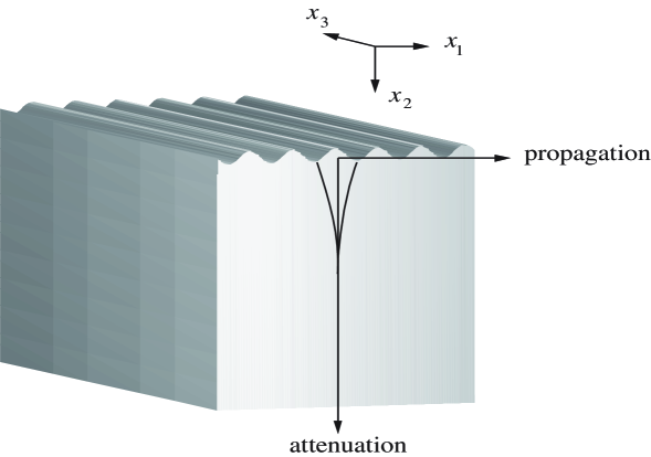
Figure 2: Incremental wave propagation localized near the surface of a semi-infinite deformed solid. The analysis does not give the amplitude nor the wavelength.

5 Governing equations

For principal waves, the fields (11) and (12) are independent of $\hat{x}_{3}=x_{3}$, because $\hat{x}_{2}=x_{2}$ and $\boldsymbol{n\cdot\hat{x}}=\hat{x}_{1}=x_{1}$. Also, recall from (2) that the non-zero components of $\boldsymbol{\mathcal{A}_{0}}$ in the ($x_{1},x_{2},x_{3}$) coordinate system of principal axes are

$$\mathcal{A}_{01111}=\lambda_{1}^{2}W_{11},\quad\mathcal{A}_{01122}=\lambda_{1}\lambda_{2}W_{12},\quad\mathcal{A}_{02222}=\lambda_{2}^{2}W_{22},$$

$$\lambda_{1}^{-2}\mathcal{A}_{01212}=\lambda_{2}^{-2}\mathcal{A}_{02121}=\dfrac{\lambda_{1}W_{1}-\lambda_{2}W_{2}}{\lambda_{1}^{2}-\lambda_{2}^{2}},\quad\mathcal{A}_{01221}=\dfrac{\lambda_{2}W_{1}-\lambda_{1}W_{2}}{\lambda_{1}^{2}-\lambda_{2}^{2}}\lambda_{1}\lambda_{2},$$ (32)

and also $\mathcal{A}_{03333}$, $\mathcal{A}_{01133}$, $\mathcal{A}_{02233}$, $\mathcal{A}_{01313}$, $\mathcal{A}_{02323}$, $\mathcal{A}_{03131}$, $\mathcal{A}_{03232}$, $\mathcal{A}_{01331}$, and $\mathcal{A}_{02332}$, whose expressions are not needed in this Section.

From these observations follows that the third equation of motion (10)₃ reduces to

$$-S_{13}+\textrm{i}S^{\prime}_{23}=-\rho v^{2}U_{3},$$ (33)

where by (7),

$$\textrm{i}S_{13}=\textrm{i}\mathcal{A}_{01313}U_{3},\qquad\textrm{i}S_{23}=\mathcal{A}_{02323}U_{3}^{\prime}.$$ (34)

Hence the movement along the $x_{3}$ principal axis is governed by an equation which depends only on $U_{3}$. For this equation, governing what is termed the anti-plane motion, we take the trivial solution: $U_{3}=0$, and we focus on the in-plane motion. According to (10)_1,2,4, it is governed by

$$-S_{11}+\textrm{i}S^{\prime}_{21}=-\rho v^{2}U_{1},\qquad-S_{12}+\textrm{i}S^{\prime}_{22}=-\rho v^{2}U_{2},\qquad\textrm{i}U_{1}+U^{\prime}_{2}=0,$$ (35)

where by (7),

$$\textrm{i}S_{11}=\textrm{i}(\mathcal{A}_{01111}+p)U_{1}+\mathcal{A}_{01122}U^{\prime}_{2}-P,$$

$$\textrm{i}S_{21}=\mathcal{A}_{02121}U^{\prime}_{1}+\textrm{i}(\mathcal{A}_{01221}+p)U_{2},$$

$$\textrm{i}S_{12}=(\mathcal{A}_{01221}+p)U^{\prime}_{1}+\textrm{i}\mathcal{A}_{01212}U_{2},$$

$$\textrm{i}S_{22}=\textrm{i}\mathcal{A}_{01122}U_{1}+(\mathcal{A}_{02222}+p)U^{\prime}_{2}-P.$$ (36)

We eliminate $p$ in favour of the pre-stress: by (6) at $j=2$, we have $p=\lambda_{2}W_{2}-\sigma_{2}$ and so by (5),

$$\mathcal{A}_{01221}+p=\mathcal{A}_{02121}-\sigma_{2}.$$ (37)

It then follows from the second equation above that

$$U^{\prime}_{1}=\textrm{i}\left[-\dfrac{\mathcal{A}_{02121}-\sigma_{2}}{\mathcal{A}_{02121}}U_{2}+\dfrac{1}{\mathcal{A}_{02121}}S_{21}\right],$$ (38)

and this constitutes the first line of the first-order system (13). The second line comes from the incremental incompressibility constraint (35)₃ as

$$U^{\prime}_{2}=\textrm{i}\left[-U_{1}\right].$$ (39)

Proceeding similarly for $S^{\prime}_{21}$, $S^{\prime}_{22}$, we find eventually that the governing equations are indeed in the form (13), where $\boldsymbol{\xi}=[U_{1},U_{2},S_{21},S_{22}]^{t}$ and $-\boldsymbol{N}_{1}$, $\boldsymbol{N}_{2}$, and $-\boldsymbol{N}_{3}$ are given by

$$\begin{bmatrix}0&\dfrac{\gamma_{21}-\sigma_{2}}{\gamma_{21}}\\ 1&0\end{bmatrix},\quad\begin{bmatrix}\dfrac{1}{\gamma_{21}}&0\\ 0&0\end{bmatrix},\quad\begin{bmatrix}2(\beta_{12}+\gamma_{21}-\sigma_{2})&0\\ 0&\gamma_{12}-\dfrac{(\gamma_{21}-\sigma_{2})^{2}}{\gamma_{21}}\end{bmatrix},$$ (40)

respectively, where we used the following short-hand notations (no sums),

$$\gamma_{ij}=\mathcal{A}_{0ijij}=\lambda_{i}^{2}\lambda_{j}^{-2}\gamma_{ji},$$

$$2\beta_{ij}=\mathcal{A}_{0iiii}+\mathcal{A}_{0jjjj}-2\mathcal{A}_{0iijj}-2\mathcal{A}_{0ijji}=2\beta_{ji}.$$ (41)

or equivalently,

$$\gamma_{ij}=(\lambda_{i}W_{i}-\lambda_{j}W_{j})\lambda_{i}^{2}/(\lambda_{i}^{2}-\lambda_{j}^{2})=\lambda_{i}^{2}\lambda_{j}^{-2}\gamma_{ji},$$

$$2\beta_{ij}=\lambda_{i}^{2}W_{ii}-2\lambda_{i}\lambda_{j}W_{ij}+\lambda_{j}^{2}W_{jj}+2(\lambda_{i}W_{j}-\lambda_{j}W_{i})\lambda_{i}\lambda_{j}/(\lambda_{i}^{2}-\lambda_{j}^{2})=2\beta_{ji}.$$ (42)

6 Resolution

The propagation condition (16) reduces to a quadratic in $q^{2}$,

$$\gamma_{21}q^{4}+(2\beta_{12}-\rho v^{2})q^{2}+\gamma_{12}-\rho v^{2}=0.$$ (43)

Notice how $\sigma_{2}$, though present in $\boldsymbol{N}$, does not appear explicitly in this equation.

Calling $q_{1}^{2}$, $q_{2}^{2}$, the roots of the quadratic, we have

$$q_{1}^{2}q_{2}^{2}=\dfrac{\gamma_{12}-\rho v^{2}}{\gamma_{21}},\quad q_{1}^{2}+q_{2}^{2}=-\dfrac{2\beta_{12}-\rho v^{2}}{\gamma_{21}}.$$ (44)

The roots $q_{1}$, $q_{2}$ of the biquadratic satisfying the decay condition (17) are in one of the two following forms; either: $q_{1}=\textrm{i}\beta_{1}$, $q_{2}=\textrm{i}\beta_{2}$, where $\beta_{1}>0$, $\beta_{2}>0$, or: $q_{1}=\alpha+\textrm{i}\beta$, $q_{2}=-\alpha+\textrm{i}\beta$, where $\beta>0$. Whatever the case, $q_{1}^{2}q_{2}^{2}>0$, $q_{1}q_{2}<0$, and $q_{1}+q_{2}$ is a purely imaginary quantity. From the first inequality we deduce that (Dowaikh and Ogden, 1990)

$$\eta=\sqrt{\dfrac{\gamma_{12}-\rho v^{2}}{\gamma_{21}}}$$ (45)

is a real quantity. From the second, and using the definitions of $\eta$ and $\gamma_{ij}$, we find

$$q_{1}q_{2}=-\eta,\quad(q_{1}+q_{2})^{2}=\dfrac{\gamma_{12}-2\beta_{12}}{\gamma_{21}}-2\eta-\eta^{2}=\lambda_{1}^{2}\lambda_{2}^{-2}-2\dfrac{\beta_{12}}{\gamma_{21}}-2\eta-\eta^{2}.$$ (46)

We compute the eigenvectors $\boldsymbol{\zeta}^{1}$ and $\boldsymbol{\zeta}^{2}$ of $\boldsymbol{N}$ corresponding to $q_{1}$ and $q_{2}$ as any column of the matrix adjoint to $\boldsymbol{N}-q_{1}\boldsymbol{I}$ and to $\boldsymbol{N}-q_{2}\boldsymbol{I}$, respectively. Choosing the third column, we find

$$\boldsymbol{\zeta}^{1}=\begin{bmatrix}\boldsymbol{a}^{1}\\ \boldsymbol{b}^{1}\end{bmatrix},\quad\boldsymbol{\zeta}^{2}=\begin{bmatrix}\boldsymbol{a}^{2}\\ \boldsymbol{b}^{2}\end{bmatrix},$$ (47)

where

$$\boldsymbol{a}^{j}=\left[-\dfrac{q_{j}^{2}}{\gamma_{21}},\dfrac{q_{j}}{\gamma_{21}}\right]^{t},\quad\boldsymbol{b}^{j}=\left[-q_{j}(q_{j}^{2}-1+\overline{\sigma}_{2}),q_{j}^{2}(1-\overline{\sigma}_{2})-\eta^{2}\right]^{t},$$ (48)

and $\overline{\sigma}_{2}=\sigma_{2}/\gamma_{21}$ is a non-dimensional measure of the pre-stress.

We can now construct the $\boldsymbol{A}=[\boldsymbol{a}^{1}|\boldsymbol{a}^{2}]$ and $\boldsymbol{B}=[\boldsymbol{b}^{1}|\boldsymbol{b}^{2}]$ matrices, and the surface impedance matrix $\boldsymbol{M}=-\textrm{i}\boldsymbol{BA}^{-1}$. It turns out to be

$$\boldsymbol{M}=-\textrm{i}\gamma_{21}\begin{bmatrix}q_{1}+q_{2}&1-\overline{\sigma}_{2}-\eta\\ -(1-\overline{\sigma}_{2}-\eta)&(q_{1}+q_{2})\eta\end{bmatrix},$$ (49)

which is indeed Hermitian because $q_{1}+q_{2}$ is a purely imaginary quantity and $\eta$ is real.

For Rayleigh surface waves, the secular equation is (22), or here, using (46),

$$\eta^{3}+\eta^{2}+(2-\lambda_{1}^{2}\lambda_{2}^{-2}+2\dfrac{\beta_{12}}{\gamma_{21}}-2\overline{\sigma}_{2})\eta-(1-\overline{\sigma}_{2})^{2}=0.$$ (50)

Dowaikh and Ogden (1990) established this form of the secular equation for principal surface waves in pre-stressed incompressible solids, following other works by Hayes and Rivlin (1961), Flavin (1963), Willson (1973a, b), Chadwick and Jarvis (1979a), Guz (2002, review with an extensive bibliography), and many others. It is of course consistent with Lord Rayleigh’s own analysis of surface waves in linear isotropic incompressible solids. To check this, let the solid be un-stressed ($\sigma_{i}=0$) and un-deformed ($\lambda_{i}=1$); then $\eta$ reduces to $\sqrt{1-\rho v^{2}/\mu_{0}}$, where $\mu_{0}$ is the infinitesimal shear modulus; also, $\beta_{12}=\gamma_{21}$ and $\eta$ is the real root of $\eta^{3}+\eta^{2}+3\eta-1=0$, that is $\eta\simeq 0.2956$ giving $\rho v^{2}/\mu_{0}\simeq 0.9126$, as found by Rayleigh (1885).

For Stoneley interface waves, the secular equation is (23) where

$$\boldsymbol{M+M}^{*}=-\textrm{i}\begin{bmatrix}\gamma_{21}(q_{1}+q_{2})-\gamma_{21}^{*}(q_{1}^{*}+q_{2}^{*})&\gamma_{21}(1-\eta)-\gamma_{21}^{*}(1-\eta^{*})\\ -\gamma_{21}(1-\eta)+\gamma_{21}^{*}(1-\eta^{*})&\gamma_{21}(q_{1}+q_{2})\eta-\gamma^{*}_{21}(q_{1}^{*}+q_{2}^{*})\eta^{*}\end{bmatrix}.$$ (51)

This equation was studied in great detail by Dowaikh and Ogden (1991) and by Chadwick (1995). It is consistent with the analysis of Stoneley (1924) of interface waves in linear isotropic incompressible solids. A remarkable feature of this secular equation for principal Stoneley interface waves in deformed incompressible solids – first noted by Chadwick and Jarvis (1979b) – is that the pre-stress $\sigma_{2}$ does not appear explicitly in it, in contrast to the equation for surface waves (50). This quantity, which is continuous across the interface ($\sigma_{2}=\sigma_{2}^{*}$), disappears in the addition of the two surface impedance matrices. Of course it still plays an implicit role, in determining the pre-strain.

Dowaikh and Ogden (1990, 1991), Chadwick (1995), and Guz (2002, review) have covered almost every aspect of principal interface wave propagation and more information can be found in their respective articles. In the next Subsection we rapidly work out two examples of surface waves.

7 Examples

First we present an example taken from the literature on elastomers, where the Mooney-Rivlin strain energy function is often encountered. It is given by

$$W=\mathcal{D}_{1}(\lambda_{1}^{2}+\lambda_{2}^{2}+\lambda_{3}^{2}-3)/2+\mathcal{D}_{2}(\lambda_{1}^{2}\lambda_{2}^{2}+\lambda_{2}^{2}\lambda_{3}^{2}+\lambda_{3}^{2}\lambda_{1}^{2}-3)/2,$$ (52)

where $\mathcal{D}_{1}$ and $\mathcal{D}_{2}$ are positive constants with the dimensions of a stiffness. The Mooney-Rivlin material enjoys special properties with respect to wave propagation (the neo-Hookean material, which corresponds to the special case $\mathcal{D}_{2}=0$, enjoys even more special properties as is seen in Section 13). For instance, once subjected to a large homogeneous pre-strain, it permits the propagation of bulk waves in every direction; these waves can be infinitesimal, but also of arbitrary finite amplitude (Boulanger and Hayes, 1992); they can be homogeneous plane waves but also inhomogeneous plane waves (Destrade, 2000, 2002). The quantities (5) are also quite special; they are

$$\gamma_{ij}=(\mathcal{D}_{1}+\mathcal{D}_{2}\lambda_{k}^{2})\lambda_{i}^{2},\quad 2\beta_{ij}=(\mathcal{D}_{1}+\mathcal{D}_{2}\lambda_{k}^{2})(\lambda_{i}^{2}+\lambda_{j}^{2}),$$ (53)

where $k\neq i,j$, and thus they satisfy

$$2\beta_{ij}=\gamma_{ij}+\gamma_{ji}.$$ (54)

These relationships mean that the biquadratic (43) factorizes to

$$(q^{2}+1)(q^{2}+\eta^{2})=0,$$ (55)

and that the secular equation (50) reduces to

$$\eta^{3}+\eta^{2}+(3-2\overline{\sigma}_{2})\eta-(1-\overline{\sigma}_{2})^{2}=0.$$ (56)

Hence one qualifying root is $q_{1}=\textrm{i}$, whatever the values of the material constants $\mathcal{D}_{1}$ and $\mathcal{D}_{2}$. The other root is $q_{2}=\textrm{i}\eta$. When there is no pre-stress normal to the boundary ($\overline{\sigma}_{2}=0$), then $\eta$ is the real root of $\eta^{3}+\eta^{2}+3\eta-1=0$, that is $\eta\simeq 0.2956$ giving

$$\rho v^{2}=\gamma_{12}-\gamma_{21}\eta^{2}=(\mathcal{D}_{1}+\mathcal{D}_{2}\lambda_{3}^{2})(\lambda_{1}^{2}-0.0874\lambda_{2}^{2}),$$ (57)

a result first established by Flavin (1963). Here $q_{1}=\textrm{i}$ and $q_{2}\simeq 0.295\textrm{i}$ so that the penetration depth of the surface wave is fixed and is completely independent of the pre-strain and of the material parameters $\mathcal{D}_{1}$ and $\mathcal{D}_{2}$. We say that the penetration depth is universal relative to the class of Mooney-Rivlin materials.

The second example is taken from the biomechanics literature. From a series of uniaxial tests on human aortic aneurysms, Raghavan and Vorp (2000) deduced that the following strain energy density gave a satisfying fit with the data plots,

$$W=\mathcal{C}_{1}(\lambda_{1}^{2}+\lambda_{2}^{2}+\lambda_{3}^{2}-3)+\mathcal{C}_{2}(\lambda_{1}^{2}+\lambda_{2}^{2}+\lambda_{3}^{2}-3)^{2},$$ (58)

where, typically, $\mathcal{C}_{1}=0.175$ MPa, $\mathcal{C}_{2}=1.9$ MPa (Karduna et al. (1997) use the same expression to model the response of passive myocardium.) A uniaxial pre-stress is $\sigma_{1}\neq 0$, $\sigma_{2}=\sigma_{3}=0$, leading through (6) to the following equi-biaxial pre-strain,

$$\lambda_{1}=\lambda,\quad\lambda_{2}=\lambda^{-1/2},\quad\lambda_{3}=\lambda^{-1/2},$$ (59)

where $\lambda$ is calculated from

$$\sigma_{1}=2(\lambda^{2}-\lambda^{-1})[\mathcal{C}_{1}+2\mathcal{C}_{2}(2-3\lambda^{-1}+\lambda^{-3})].$$ (60)

Finally, using the following expressions for the relevant moduli,

$$\gamma_{21}=2\mathcal{C}_{1}\lambda^{-1}+4\mathcal{C}_{2}(2\lambda^{-1}-3\lambda^{-2}+\lambda^{-4}),\qquad\gamma_{12}=\lambda^{3}\gamma_{21},$$

$$\beta_{21}=\mathcal{C}_{1}(\lambda^{2}+\lambda^{-1})+2\mathcal{C}_{2}(4\lambda^{2}-3\lambda-\lambda^{-1}-3\lambda^{-2}+3\lambda^{-4}),$$ (61)

it is a simple matter to solve the secular equation (50) numerically and plot the variations of the squared wave speed, scaled with respect to the squared bulk wave speed $\gamma_{12}/\rho$, with the pre-stretch $\lambda$. Figure 3$b$ displays these variations; for comparison purposes, Figure 3$a$ shows the variations of the scaled squared wave speed in the case of a Mooney-Rivlin material in uniaxial stress; in that later case the graph is independent of the material parameters $\mathcal{D}_{1}$ and $\mathcal{D}_{2}$ because by (57), $\rho v^{2}/\gamma_{21}=1-0.0874\lambda^{-3}$. The dashed lines indicate the speed of Lord Rayleigh’s squared speed in the isotropic (no pre-strain) case where $\lambda=1$, $\rho v^{2}/\gamma_{12}\simeq 0.9126$. Notice how different the responses of two solids are in that neighbourhood. Note also that for high compressive stretches, the squared speeds eventually falls off to zero; this happens at $\lambda\simeq 0.0874^{1/3}\simeq 0.444$ for all Mooney-Rivlin materials, as shown by Biot (1963), and at $\lambda\simeq 0.315$ for the soft biological tissue model above. Beyond that critical compression stretch, $v^{2}<0$, leading to a purely imaginary $v$, an amplitude which then grows exponentially with time according to (11), and a breakdown of the linearized analysis. The search for critical compression stretches is an extremely active area of research, clearly linked to the geometric stability analysis of solids.

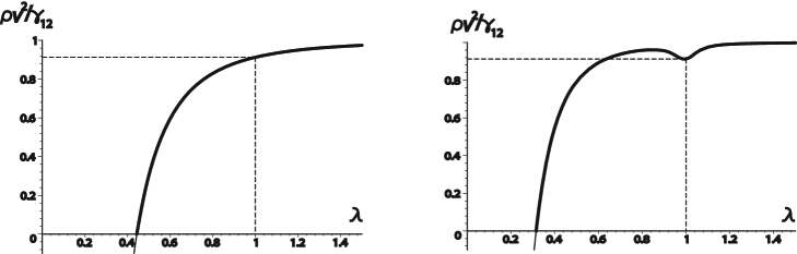
Figure 3: Variations of the scaled squared surface wave speed with the stretch in uniaxial pre-stress (a) for any Mooney-Rivlin material and (b) for the solid with strain energy density (58) where $\mathcal{C}_{1}=0.175$ MPa, $\mathcal{C}_{2}=1.9$ MPa.

Chapter 4 Waves polarized in a principal plane

In this Section we study the case where $\hat{x}_{3}$ is aligned with the principal axis $x_{3}$ but neither $\hat{x}_{1}$ (propagation direction) nor $\hat{x}_{2}$ (attenuation direction) are aligned with principal axes. The components $\hat{\mathcal{A}}_{0jilk}$ in the ($\hat{x}_{1}\hat{x}_{2}\hat{x}_{3}$) coordinate system of the instantaneous elastic moduli tensor $\boldsymbol{\mathcal{A}_{0}}$ are related to the components $\mathcal{A}_{0jilk}$, given by (5), in the ($x_{1}x_{2}x_{3}$) coordinate system of principal axes through the tensor transformations

$$\hat{\mathcal{A}}_{0jilk}=\Omega_{jp}\Omega_{iq}\Omega_{lr}\Omega_{ks}\mathcal{A}_{0pqrs},\quad\text{where}\quad\boldsymbol{\Omega}=\begin{bmatrix}\cos\Theta&-\sin\Theta&0\\ \sin\Theta&\cos\Theta&0\\ 0&0&1\end{bmatrix},$$ (62)

and $\Theta$ is the angle between $x_{1}$ and $\hat{x}_{1}$.

In particular we find that the non-zero components in the forms $\hat{\mathcal{A}}_{013lk}$ and $\hat{\mathcal{A}}_{023lk}$ are $\hat{\mathcal{A}}_{01313}$, $\hat{\mathcal{A}}_{01323}$, $\hat{\mathcal{A}}_{01331}$, $\hat{\mathcal{A}}_{02323}$, $\hat{\mathcal{A}}_{02313}$, and $\hat{\mathcal{A}}_{02332}$. The mechanical fields (11) and (12) are independent of $\hat{x}_{3}=x_{3}$ because $\boldsymbol{n\cdot\hat{x}}=\hat{x}_{1}$ here. As a consequence, the third equation of motion (10)₃ reduces to

$$-S_{13}+\textrm{i}S^{\prime}_{23}=-\rho v^{2}U_{3},$$ (63)

where by (7),

$$\textrm{i}S_{13}=\textrm{i}\hat{\mathcal{A}}_{01313}U_{3}+\hat{\mathcal{A}}_{01323}U_{3}^{\prime},\quad\textrm{i}S_{23}=\textrm{i}\hat{\mathcal{A}}_{02313}U_{3}+\hat{\mathcal{A}}_{02323}U_{3}^{\prime}.$$ (64)

Hence the movement along the $x_{3}$ principal axis is governed by an equation which depends only on $U_{3}$, and for this anti-plane motion we take the trivial solution: $U_{3}=0$.

The equations governing the in-plane motion have been derived in the case of a general plane pre-strain by Fu (2005a) and solved for surface waves in the case of a pre-strain consisting in a triaxial stretch followed by a simple shear by Destrade and Ogden (2005). Instead of treating these cases again, we revisit the case relative to one of the most important pre-strain fitting into the present context, that of finite simple shear, presented originally by Connor and Ogden (1995) for surface waves.

Figure 4 sketches what happens to a unit cube when a solid is subject to the simple shear of amount $K$,

$$\hat{x}_{1}=X_{1}+KX_{2},\quad\hat{x}_{2}=X_{2},\quad\hat{x}_{3}=X_{3}.$$ (65)

Here the principal axes are $x_{3}=X_{3}$ and $x_{1}$, $x_{2}$ which make an angle $\psi$ with $X_{1}$ and with $X_{2}$, respectively. That angle, and the corresponding principal stretches are (e.g. Chadwick (1976)),

$$\psi=(1/2)\tan^{-1}(2/K),\quad\lambda_{1,2}=\sqrt{1+K^{2}/4}\pm K/2,\quad\lambda_{3}=1.$$ (66)

These relations highlight a major difference between this homogeneous pre-strain and the triaxial pre-stretch (31): here the orientation of the principal axes with respect to the plane interface changes as the magnitude of the pre-strain changes.

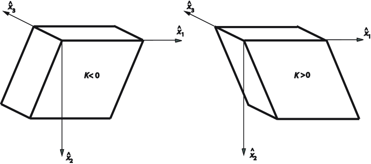
Figure 4: Finite simple shear of amount $K$ of a block near the interface. The $\hat{x}_{1}$ direction is the direction of shear; the ($\hat{x}_{1}\hat{x}_{2}$) plane is the plane of shear; the ($\hat{x}_{1}\hat{x}_{3}$) plane is the glide plane.

8 Governing equations for simple shear pre-strain

The deformation (65) is an example of plane strain. As we focus on two-partial incremental waves in this Section, we may take advantage of formulas established by Merodio and Ogden (2002) in a similar context. The components of the deformation gradient tensor $\boldsymbol{F}$ and of the left Cauchy-Green strain tensor $\boldsymbol{B}$ for 2D pre-strain and 2D incremental motions, in the ($\hat{x}_{1},\hat{x}_{2}$) coordinate system (aligned with the ($X_{1},X_{2}$) system), are

$$\boldsymbol{F}=\begin{bmatrix}1&K\\ 0&1\end{bmatrix},\qquad\boldsymbol{B}=\begin{bmatrix}1+K^{2}&K\\ K&1\end{bmatrix}.$$ (67)

For plane strain, $\lambda_{3}=1$, so that in incompressible solids $\lambda_{2}=\lambda_{1}^{-1}$ by (1). It follows by (4) that $I_{1}=I_{2}$. Accordingly, we define the single-variable function $\widehat{W}(I_{1})$ by the identity

$$\widehat{W}(I_{1})=W(I_{1},I_{1}).$$ (68)

Then the 2D version of the constitutive equation (5) is

$$\boldsymbol{\sigma}=-\hat{p}\boldsymbol{I}+2\widehat{W}_{1}\boldsymbol{B},$$ (69)

where $\hat{p}$ is the Lagrange multiplier due to the incompressibility constraint. Also, the components of $\boldsymbol{\mathcal{A}_{0}}$ are (Merodio and Ogden, 2002),

$$\hat{\mathcal{A}}_{0jilk}=2\widehat{W}_{1}\delta_{ik}B_{jl}+4\widehat{W}_{11}B_{ij}B_{lk},$$ (70)

where $\widehat{W}_{1}=\widehat{W}^{\prime}(I_{1})$, $\widehat{W}_{11}=\widehat{W}^{\prime\prime}(I_{1})$. With the help of (67)₂, we find that in the ($\hat{x}_{1},\hat{x}_{2}$) coordinate system, the non-zero components $\hat{\mathcal{A}}_{0jilk}$ relevant to in-plane motion are

$$\hat{\mathcal{A}}_{01112}=\hat{\mathcal{A}}_{01211}=4\widehat{W}_{11}K(1+K^{2}),$$

$$\hat{\mathcal{A}}_{01121}=\hat{\mathcal{A}}_{02111}=2\widehat{W}_{1}K+4\widehat{W}_{11}K(1+K^{2}),$$

$$\hat{\mathcal{A}}_{01122}=\hat{\mathcal{A}}_{02211}=4\widehat{W}_{11}(1+K^{2}), \hat{\mathcal{A}}_{01221}=\hat{\mathcal{A}}_{02112}=4\widehat{W}_{11}K^{2},$$

$$\hat{\mathcal{A}}_{01212}=2\widehat{W}_{1}(1+K^{2})+4\widehat{W}_{11}K^{2}, \hat{\mathcal{A}}_{02121}=2\widehat{W}_{1}+4\widehat{W}_{11}K^{2},$$

$$\hat{\mathcal{A}}_{01222}=\hat{\mathcal{A}}_{02212}=2\widehat{W}_{1}K+4\widehat{W}_{11}K, \hat{\mathcal{A}}_{02122}=\hat{\mathcal{A}}_{02221}=4\widehat{W}_{11}K,$$

$$\hat{\mathcal{A}}_{01111}=2\widehat{W}_{1}(1+K^{2})+4\widehat{W}_{11}(1+K^{2})^{2}, \hat{\mathcal{A}}_{02222}=2\widehat{W}_{1}+4\widehat{W}_{11}.$$ (71)

Now the remaining incremental governing equations (10)_1,2,4 reduce to

$$-S_{11}+\textrm{i}S^{\prime}_{21}=-\rho v^{2}U_{1},\quad-S_{12}+\textrm{i}S^{\prime}_{22}=-\rho v^{2}U_{2},\quad\textrm{i}U_{1}+U^{\prime}_{2}=0,$$ (72)

where by (7),

$$\textrm{i}S_{11}=\textrm{i}(\hat{\mathcal{A}}_{01111}+\hat{p})U_{1}+\textrm{i}\hat{\mathcal{A}}_{01112}U_{2}+\hat{\mathcal{A}}_{01121}U_{1}^{\prime}+\hat{\mathcal{A}}_{01122}U_{2}^{\prime}-\textrm{i}\hat{P},$$

$$\textrm{i}S_{12}=\textrm{i}\hat{\mathcal{A}}_{01112}U_{1}+\textrm{i}\hat{\mathcal{A}}_{01212}U_{2}+(\hat{\mathcal{A}}_{01221}+\hat{p})U_{1}^{\prime}+\hat{\mathcal{A}}_{01222}U_{2}^{\prime}.$$

$$\textrm{i}S_{21}=\textrm{i}\hat{\mathcal{A}}_{01121}U_{1}+\textrm{i}(\hat{\mathcal{A}}_{01221}+\hat{p})U_{2}+\hat{\mathcal{A}}_{02121}U_{1}^{\prime}+\hat{\mathcal{A}}_{02122}U_{2}^{\prime},$$

$$\textrm{i}S_{22}=\textrm{i}\hat{\mathcal{A}}_{01122}U_{1}+\textrm{i}\hat{\mathcal{A}}_{01222}U_{2}+\hat{\mathcal{A}}_{02122}U_{1}^{\prime}+(\hat{\mathcal{A}}_{02222}+\hat{p})U_{2}^{\prime}-\textrm{i}\hat{P},$$ (73)

where $\hat{P}$ is the increment of $\hat{p}$. The pre-stress necessary to maintain the solid in the static state of large simple shear is (69). In particular, the $\hat{\sigma}_{22}$ component along the $\hat{x}_{2}$ axis is found using (67) and (68) as

$$\hat{\sigma}_{22}=-\hat{p}+2\widehat{W}_{1},$$ (74)

leading to the connection

$$\hat{\mathcal{A}}_{01221}+\hat{p}=\hat{\mathcal{A}}_{02121}-\hat{\sigma}_{22}.$$ (75)

Note that Connor and Ogden (1995) and Fu (2005a) keep $\sigma_{2}$ rather than $\hat{\sigma}_{22}$ as a measure of the pre-stress. It is the component of the pre-stress along the principal axis $x_{2}$, whose orientation changes with the pre-strain, in contrast to $\hat{\sigma}_{22}$, the component of the Cauchy pre-stress tensor along the unchanged normal to the interface. As pointed out by Hussain and Ogden (2000), it is $\hat{\sigma}_{22}$ which is continuous across the interface of two bonded sheared solids.

Following the same procedure as in Section 5, we find the Stroh formulation of the governing equations in the expected form (10), where $\boldsymbol{\xi}=[U_{1},U_{2},S_{21},S_{22}]^{t}$ and $-\boldsymbol{N}_{1}$ and $\boldsymbol{N}_{2}$, are given by

$$\begin{bmatrix}K&1-\dfrac{\hat{\sigma}_{22}}{2\widehat{W}_{1}+4\widehat{W}_{11}K^{2}}\\ 1&0\end{bmatrix},\quad\begin{bmatrix}\dfrac{1}{2\widehat{W}_{1}+4\widehat{W}_{11}K^{2}}&0\\ 0&0\end{bmatrix},$$ (76)

respectively, and $-\boldsymbol{N}_{3}$ by

$$\begin{bmatrix}2(4\widehat{W}_{1}-\hat{\sigma}_{22})&-(4\widehat{W}_{1}-\hat{\sigma}_{22})K\\ -(4\widehat{W}_{1}-\hat{\sigma}_{22})K&2\widehat{W}_{1}K^{2}+2\hat{\sigma}_{22}-\dfrac{\hat{\sigma}_{22}^{2}}{2\widehat{W}_{1}+4\widehat{W}_{11}K^{2}}\end{bmatrix}.$$ (77)

9 Resolution

The propagation condition (16) reduces to a quartic in $q$,

$$2(\widehat{W}_{1}+2\widehat{W}_{11}K^{2})q^{4}+4(\widehat{W}_{1}+2\widehat{W}_{11}K^{2})Kq^{3}\\ +[2(\widehat{W}_{1}(2+K^{2})-4\widehat{W}_{11}K^{2}(2-K^{2})-\rho v^{2}]q^{2}\\ +4(\widehat{W}_{1}-2\widehat{W}_{11}K^{2})Kq\\ +2\widehat{W}_{1}(1+K^{2})+4\widehat{W}_{11}K^{2}-\rho v^{2}=0.$$ (78)

Notice how $\hat{\sigma}_{22}$, though present in $\boldsymbol{N}$, does not appear explicitly in this equation.

Quite surprisingly, there are two instances – both pointed out by Connor and Ogden (1995, 1996) – where we can solve this quartic exactly and simply. The first instance occurs for incremental deformations, when $v=0$; it is applicable whatever the strain energy density $W$ might be. The reason for the simplicity of this resolution is made apparent by the change of unknown from $q$ to $\widetilde{q}=q-K/2$. Then the quartic becomes

$$2(\widehat{W}_{1}+2\widehat{W}_{11}K^{2})\widetilde{q}^{4}+[\widehat{W}_{1}(4-K^{2})-2\widehat{W}_{11}K^{2}(4+K^{2})-\rho v^{2}]\widetilde{q}^{2}\\ +(\rho v^{2})K\widetilde{q}+[(\widehat{W}_{1}+2\widehat{W}_{11}K^{2})(4+K^{2})-2\rho v^{2}](4+K^{2})/8=0,$$ (79)

which is clearly a biquadratic at $v=0$. The consequence is that any incremental static problem can be solved in its entirety for sheared solids because the roots $q$ are accessible explicitly. This was to be expected though, because of an important theorem by Fu and Mielke (2002) which states that “the buckling condition for a pre-stressed elastic half-space is independent of the orientation of the surface as long as the surface normal remains in the ($x_{1},x_{2}$) plane”; the buckling condition is what corresponds to the marginally stable static solution obtained at $v=0$; it is also called the wrinkling condition, or the bifurcation criterion, or any other denomination associated with the onset of instability in the linearised (incremental) theory.

The second instance where the quartic is easy to solve is when the solid is a Mooney-Rivlin material, see (52); this case is treated in Section 10.

In general however, the quartic is difficult (but not impossible, see Fu (2005a, b), Destrade and Fu (2006), and the concluding Section) to solve analytically and other methods, such as those relying on the fundamental equations (25), are required. For the time being, we complete the picture with formal calculations.

Assuming the roots of the quartic have been computed, and calling them $q_{1}$, $q_{2}$, $\overline{q}_{1}$, $\overline{q}_{2}$, where $q_{1}$ and $q_{2}$ both satisfy the decay condition (17), we find that the eigenvectors $\boldsymbol{\zeta}^{1}$ and $\boldsymbol{\zeta}^{2}$ associated with $q_{1}$ and $q_{2}$, respectively, are

$$\boldsymbol{\zeta}^{1}=\begin{bmatrix}\boldsymbol{a}^{1}\\ \boldsymbol{b}^{1}\end{bmatrix},\quad\boldsymbol{\zeta}^{2}=\begin{bmatrix}\boldsymbol{a}^{2}\\ \boldsymbol{b}^{2}\end{bmatrix},$$ (80)

where

$$\boldsymbol{a}^{j}=[q_{j}^{2},-q_{j}]^{t},$$

$$\boldsymbol{b}^{j}=\left[q_{j}\left(\hat{\gamma}_{21}(q_{j}^{2}+Kq_{j}-1)+\hat{\sigma}_{22}\right),-(\hat{\gamma}_{21}-\hat{\sigma}_{22})q_{j}^{2}+\hat{\nu}_{12}q_{j}+\hat{\gamma}_{12}-\rho v^{2}\right]^{t}.$$ (81)

Here,

$$\hat{\gamma}_{21}=2\widehat{W}_{1}+4\widehat{W}_{11}K^{2}, \hat{\gamma}_{12}=2\widehat{W}_{1}(1+K^{2})+4\widehat{W}_{11}K^{2},$$

$$\hat{\beta}_{12}=\widehat{W}_{1}(2+K^{2})-2\widehat{W}_{11}K^{2}(2-K^{2}), \hat{\nu}_{12}=2\widehat{W}_{1}K-4\widehat{W}_{11}K^{3}.$$ (82)

Then we compute the $\boldsymbol{A}=[\boldsymbol{a}^{1}|\boldsymbol{a}^{2}]$ and $\boldsymbol{B}=[\boldsymbol{b}^{1}|\boldsymbol{b}^{2}]$ matrices, and eventually the surface impedance matrix $\boldsymbol{M}=-\textrm{i}\boldsymbol{BA}^{-1}$, as

$$\boldsymbol{M}=-\textrm{i}\begin{bmatrix}\hat{\gamma}_{21}(K+q_{1}+q_{2})&\hat{\gamma}_{21}(1+q_{1}q_{2})+\hat{\sigma}_{22}\vspace{6pt}\\ \dfrac{\rho v^{2}-\hat{\gamma}_{12}}{q_{1}q_{2}}-\hat{\gamma}_{21}-\hat{\sigma}_{22}&(\rho v^{2}-\hat{\gamma}_{12})\dfrac{q_{1}+q_{2}}{q_{1}q_{2}}-\hat{\nu}_{12}\end{bmatrix}.$$ (83)

Note that this matrix is indeed Hermitian; this is easy to show by using the quartic (78) and the definitions (9) to uncover the identities:

$$q_{1}+q_{2}+\overline{q}_{1}+\overline{q}_{2}=-2K,$$

$$q_{1}q_{2}\overline{q}_{1}\overline{q}_{2}=(\hat{\gamma}_{12}-\rho v^{2})/\hat{\gamma}_{21},$$

$$q_{1}q_{2}(\overline{q}_{1}+\overline{q}_{2})+\overline{q}_{1}\overline{q}_{2}(q_{1}+q_{2})=-2\hat{\nu}_{12}/\hat{\gamma}_{21}.$$ (84)

These identities allow us to rewrite the surface impedance matrix as

$$\boldsymbol{M}=-\textrm{i}\begin{bmatrix}\hat{\gamma}_{21}(q_{1}+q_{2}-\overline{q}_{1}-\overline{q}_{2})/2&\hat{\gamma}_{21}(1+q_{1}q_{2})-\hat{\sigma}_{22}\vspace{6pt}\\ -\hat{\gamma}_{21}(1+\overline{q}_{1}\overline{q}_{2})+\hat{\sigma}_{22}&-\hat{\gamma}_{21}[q_{1}q_{2}(\overline{q}_{1}+\overline{q}_{2})-\overline{q}_{1}\overline{q}_{2}(q_{1}+q_{2})]/2\end{bmatrix}.$$ (85)

Fu (2005a) derived the same form of the surface impedance matrix for the more general case of any plane strain (any pre-strain where $\lambda_{3}=1$), which includes the present case of finite shear.

Notice also how the pre-stress $\hat{\sigma}_{22}$ is going to be explicitly present in the secular equation for Rayleigh surface waves (22), but absent from the secular equation for Stoneley interface waves (23). These secular equations remain implicit as long as the roots $q_{1}$ and $q_{2}$ are not known. In the general case where the quartic (78) is not solvable in a simple manner, we seek an explicit secular equation using the fundamental equations (25).

Rayleigh surface waves.

With the explicit expressions (76) and (77) for the blocks of the matrix $\boldsymbol{N}$, we can compute $\boldsymbol{N}^{-1}$ and $\boldsymbol{N}^{2}$. The lower left corner of these gives in turn $\boldsymbol{K}^{(1)}=\boldsymbol{N}_{3}+\rho v^{2}\boldsymbol{I}$ and $\boldsymbol{K}^{(-1)}$, $\boldsymbol{K}^{(2)}$, respectively. Then the equations (30) written at $n=1,-1,2$, yield the linear homogeneous system

$$\begin{bmatrix}K^{(1)}_{11}&K^{(1)}_{12}&K^{(1)}_{22}\\ K^{(-1)}_{11}&K^{(-1)}_{12}&K^{(-1)}_{22}\\ K^{(2)}_{11}&K^{(2)}_{12}&K^{(2)}_{22}\end{bmatrix}\begin{bmatrix}U_{1}(0)\overline{U}_{1}(0)\\ U_{1}(0)\overline{U}_{2}(0)+\overline{U}_{1}(0)U_{2}(0)\\ U_{2}(0)\overline{U}_{2}(0)\end{bmatrix}=\begin{bmatrix}0\\ 0\\ 0\end{bmatrix}.$$ (86)

The vanishing of the determinant of the $3\times 3$ matrix on the left hand side is the explicit polynomial secular equation for surface waves in a sheared incompressible semi-infinite solid. It is a polynomial of degree 4 in $\rho v^{2}$. It is too long to reproduce in general but easy to obtain (and solve numerically) with a computer algebra system. Here we present its expression in the case where $\hat{\sigma}_{22}=0$. Then, $\boldsymbol{K}^{(1)}$ and $\boldsymbol{K}^{(2)}$ are given by

$$\begin{bmatrix}\rho v^{2}-8\widehat{W}_{1}&4\widehat{W}_{1}\\ 4\widehat{W}_{1}&\rho v^{2}+2\widehat{W}_{1}\end{bmatrix},\quad\begin{bmatrix}2(4\widehat{W}_{1}-\rho v^{2})K&2\widehat{W}_{1}(4-K^{2})-2\rho v^{2}\\ 2\widehat{W}_{1}(4-K^{2})-2\rho v^{2}&-8\widehat{W}_{1}K\end{bmatrix},$$ (87)

respectively, the components of $\boldsymbol{K}^{(-1)}$ are

$$K^{(-1)}_{11}=2(2\widehat{W}_{1}-\rho v^{2}),$$

$$K^{(-1)}_{12}=-2[2\widehat{W}_{1}(1+K^{2})-\rho v^{2}]K,$$

$$K^{(-1)}_{22}=4\widehat{W}_{1}(2+K^{2})^{2}+\rho v^{2}\dfrac{\rho v^{2}-2\widehat{W}_{1}(5+K^{2})-4\widehat{W}_{11}K^{2}(1+K^{2})}{\widehat{W}_{1}+2\widehat{W}_{11}K^{2}},$$ (88)

(up to an inessential common factor), and the secular equation is the quartic

$$x^{4}-5x^{3}+\left(8\dfrac{5+K^{2}}{4+K^{2}}+K^{2}\dfrac{\widehat{W}_{11}}{\widehat{W}_{1}}\right)x^{2}\\ -8\left(4\dfrac{1+K^{2}}{4+K^{2}}+K^{2}\dfrac{\widehat{W}_{11}}{\widehat{W}_{1}}\right)x+8\dfrac{\widehat{W}_{1}+2\widehat{W}_{11}K^{2}}{\widehat{W}_{1}(4+K^{2})}=0,$$ (89)

where $x$ is the following non-dimensional measure of the squared wave speed, $x=\rho v^{2}/[\widehat{W}_{1}(4+K^{2})]$.

As stated above, the secular equation is also a quartic in the squared wave speed when $\hat{\sigma}_{22}\neq 0$. For a given material, a given pre-stress, and a given shear, its numerical resolution may yield more than one positive real root. If such is the case, then for each corresponding speed, compute the roots to the quartic (78) and discard those (supersonic) speeds which do not give two complex conjugate pairs of roots. Finally, find which of the remaining speeds (if there is more than one) satisfies the secular equation written in optimal form (22).

Stoneley shear-twin interface waves.

For Stoneley interface waves, the fundamental equations (25) are not practical to derive secular equations in general, and we must resort to other methods, such as those developed by Destrade and Fu (2006). The exception is the special case when each half-space is filled with Mooney-Rivlin materials, because then the roots to the quartic (78) can be found easily, see Section 10.

We now focus on the possibility of propagating incremental waves at a shear-twin interface. In this configuration, two solids, made of the same incompressible material, are subject to equal and opposite shears, see Figure 5. The study of wave propagation at this type of interface can have important repercussions in the non-destructive evaluation of a twinned interface because this bimaterial can “simulate the finite (plastic) deformation associated with a crystal twin” (Hussain and Ogden, 2000).

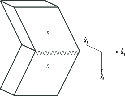
Figure 5: Stoneley wave propagation at a shear-twin interface. Both half-spaces are occupied with the same incompressible solid, one subject to a simple shear of amount $K$, the other subject to a simple shear of amount $-K$. The analysis shows that Stoneley waves cannot actually travel in the direction of shear.

For one half-space, the propagation condition is the quartic (78). For the other half-space, the amount of shear is changed to its opposite, but $\widehat{W}_{1}$ and $\widehat{W}_{11}$ do not change signs because they are functions of $K^{2}$. It follows that if $q_{1}$ and $q_{2}$ are qualifying roots of the propagation condition in one half-space, then $-q_{1}$ and $-q_{2}$ are qualifying roots in the other half-space. Also, we see from (9) that $\hat{\gamma}_{21}$, $\hat{\gamma}_{12}$, and $\hat{\beta}_{21}$ in one half-space are equal to their counterparts in the other half-space, but that the counterpart to $\hat{\nu}_{12}$ is $-\hat{\nu}_{12}$. Finally, $\hat{\sigma}_{22}$ is continuous across the interface. Then we conclude from (9) that the counterparts to the matrices

$$\boldsymbol{A}=\begin{bmatrix}A_{11}&A_{12}\\ A_{21}&A_{22}\end{bmatrix},\qquad\boldsymbol{B}=\begin{bmatrix}B_{11}&B_{12}\\ B_{21}&B_{22}\end{bmatrix},$$ (90)

in one half-space are the matrices (Destrade, 2003; Ting, 2005)

$$\boldsymbol{A}^{*}=\begin{bmatrix}A_{11}&A_{12}\\ -A_{21}&-A_{22}\end{bmatrix},\qquad\boldsymbol{B}^{*}=\begin{bmatrix}-B_{11}&-B_{12}\\ B_{21}&B_{22}\end{bmatrix},$$ (91)

in the other half-space. In turn, this conclusion leads to the following sum of surface impedance matrices

$$\boldsymbol{M}+\boldsymbol{M}^{*}=\begin{bmatrix}2M_{11}&0\vspace{6pt}\\ 0&2M_{22}\end{bmatrix},$$ (92)

where $\boldsymbol{M}^{*}=\textrm{i}\boldsymbol{B}^{*}(\boldsymbol{A}^{*})^{-1}$. Consequently, the exact secular equation for Stoneley shear-twin interface waves is, according to (23), (85), and (92) that either

$$\Im(q_{1}+q_{2})=0,\quad\text{or}\quad\Im[q_{1}q_{2}(\overline{q}_{1}+\overline{q}_{2})]=0.$$ (93)

However, as is easily proved, neither of these quantities can be zero when both $q_{1}$ and $q_{2}$ have positive imaginary parts. It follows that Stoneley waves cannot propagate in the direction of sheared at a shear-twin interface, whatever the strain energy function is, and whatever what the shear is. Note however that Hussain and Ogden (2000) show, in their study of reflection and transmission of plane waves at shear-twin interface, that an incident harmonic plane wave can give rise to an interfacial wave (but of a different type than the Stoneley type).

10 Examples

Sheared Mooney-Rivlin solids.

For the Mooney-Rivlin strain energy density (52) we have

$$\widehat{W}_{1}=\mathcal{D}/2,\qquad\widehat{W}_{11}=0,$$ (94)

where $\mathcal{D}=\mathcal{D}_{1}+\mathcal{D}_{2}$ is the shear modulus. The quartic propagation condition (78) then factorizes to

$$(q^{2}+1)(q^{2}+2Kq+K^{2}+\eta^{2})=0,\quad\text{where}\quad\eta=\sqrt{1-\rho v^{2}/\mathcal{D}},$$ (95)

and its roots with positive imaginary parts are

$$q_{1}=\textrm{i},\qquad q_{2}=-K+\textrm{i}\eta.$$ (96)

We also have

$$\hat{\gamma}_{21}=\mathcal{D},\quad\hat{\gamma}_{12}=\mathcal{D}(1+K^{2}),\quad\hat{\beta}_{12}=\mathcal{D}(2+K^{2}),\quad\hat{\nu}_{12}=\mathcal{D}K,$$ (97)

and the surface impedance matrix of (85) reduces to

$$\boldsymbol{M}=\mathcal{D}\begin{bmatrix}\eta+1&-K+\textrm{i}(\eta-1)+\textrm{i}\hat{\sigma}_{22}/\mathcal{D}\vspace{6pt}\\ -K-\textrm{i}(\eta-1)-\textrm{i}\hat{\sigma}_{22}/\mathcal{D}&\eta^{2}+\eta+K^{2}\end{bmatrix}.$$ (98)

For Rayleigh surface waves in a sheared Mooney-Rivlin material, the secular equation (22) is a cubic in $\eta$,

$$\eta^{3}+\eta^{2}+(3+K^{2}-2\hat{\sigma}_{22}/\mathcal{D})\eta-(1-\hat{\sigma}_{22}/\mathcal{D})^{2}=0.$$ (99)

See Connor and Ogden (1995) for this equation with $\sigma_{2}$ instead of $\hat{\sigma}_{22}$, and Destrade and Ogden (2005) for a generalization of this equation to a triaxial stretch followed by a shear. See also Figure 6 for the variations of the squared scaled wave speed $\rho v^{2}/\mathcal{D}=1-\eta^{2}$ with the amount of shear $K$, for several values of the pre-stress $\hat{\sigma}_{22}$. In particular, the plots at $\hat{\sigma}_{22}=\pm 2\mathcal{D}$ show that the Mooney-Rivlin material is unstable when subject only to a hydrostatic pressure of that amount (that is, $\rho v^{2}=0$ at $K=0$) but regains stability as soon as it is sheared ($\rho v^{2}>0$ at $K\neq 0$) .

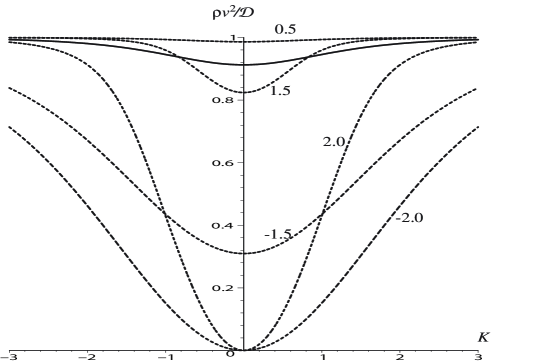
Figure 6: Squared scaled surface wave speed $\rho v^{2}/\mathcal{D}$ as a function of the amount of shear $K$ for a Mooney-Rivlin material. For the solid plot, there is no pre-stress normal to the boundary ($\hat{\sigma}_{22}=0$); for the dashed plots, the displayed number indicates the value of the non-dimensional pre-stress $\hat{\sigma}_{22}/\mathcal{D}$. More plots are found in the article by Connor and Ogden (1995).

As is clear from the roots (96), from the secular equation (99), and from Figure 6, both the penetration depth and the speed are even functions of $K$. Also, once $\eta$ is found by solving the secular equation, we have $\partial\eta/\partial(K^{2})=-\eta^{2}/[2\eta^{3}+\eta^{2}+(1-\hat{\sigma}_{22}/\mathcal{D})^{2}]<0$ and $\partial\Im(q_{2})/\partial(K^{2})=\partial\eta/\partial(K^{2})<0$, indicating that both the surface wave speed and the penetration depth increase with the magnitude of the shear.

We note that having found an explicit expression (98) for the surface impedance matrix allows us to solve the problem of Stoneley interface waves in its entirety, for half-spaces made of different Mooney-Rivlin solids, subject to different amounts of shear; see Chadwick and Jarvis (1979b) for more discussion on this point.

Sheared Gent solids.

As an example of a strain energy density for which the quartic (78) is not easily solved, we now work with the following function,

$$W=-\textstyle{\frac{1}{2}}\mathcal{C}J_{m}\ln\left(1-\dfrac{I_{1}-3}{J_{m}}\right),\qquad I_{1}<3+J_{m},$$ (100)

proposed initially by Gent (1996) to describe strain-stiffening elastomers and since then extensively used by Horgan and Saccomandi (2003, and references therein) to model strain-stiffening soft biological tissues such as arteries. Here $\mathcal{C}>0$ is the infinitesimal shear modulus and $J_{m}>0$ is a constant, accounting for the limiting chain extensibility of the solid. Hence the condition (100)₂ limits the amount of shear by imposing

$$-\sqrt{J_{m}}<K<\sqrt{J_{m}}.$$ (101)

Turning our attention to the propagation of surface waves, we compute the following quantities,

$$\widehat{W}_{1}=\dfrac{\mathcal{C}J_{m}}{2(J_{m}-K^{2})},\qquad\widehat{W}_{11}=\dfrac{\mathcal{C}J_{m}}{2(J_{m}-K^{2})^{2}}.$$ (102)

To fix the ideas, we take two Gent materials, one with $J_{m}=9.0$, the other (stiffer) with $J_{m}=1.0$. Figure 7 shows the variations of the non-dimensional measure of the surface wave speed $\sqrt{\rho v^{2}/\mathcal{C}}$ with the amount of shear $K$. The bounds due to the inequalities (101) are clearly visible, indicating that the solids become more and more rigid as their limit of chain extensibility is approached. The speed is an even function of $K$ and only the $K\geqslant 0$ needs be displayed. For a boundary free of pre-stress ($\hat{\sigma}_{22}=0$), we solve numerically the quartic secular equation (89) and find in general that there is two real positive roots for $\rho v^{2}$; one gives a supersonic speed and is discarded; the other gives a speed for which the exact secular equation (22) is satisfied and it is kept. The Figure also shows (dotted plots) the effect of the compressive pre-stress $\hat{\sigma}_{22}=-1.5\mathcal{C}$, which is to slow the wave down in the small-to-moderate shear region; here again a quartic secular equation is solved numerically and only one speed is kept.

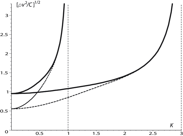
Figure 7: Scaled surface wave speed $\sqrt{\rho v^{2}/\mathcal{C}}$ as a function of the amount of shear $K$ for two Gent materials. For the solid plots, there is no pre-stress normal to the boundary ($\hat{\sigma}_{22}=0$); for the dashed plots, the pre-stress is $\hat{\sigma}_{22}=-1.5\mathcal{C}$. The vertical asymptotes correspond to the maximal amount of shear, that is $K_{\text{max}}=\pm 3.0$ for the Gent solid with $J_{m}=9.0$, and $K_{\text{max}}=\pm 1.0$ for the other, stiffer, Gent solid with $J_{m}=1.0$.

Chapter 5 Propagation in a principal plane

In this Section we consider an interface wave propagating in a principal plane, $x_{2}=0$ say, but not in a principal direction. We call $\theta$ the angle between the propagation direction $\hat{x}_{1}$ and the principal axis $x_{1}$, see Figure 8. Although some results exist for non-principal Stoneley waves (Destrade, 2005), the focus of this Section is on Rayleigh surface waves.

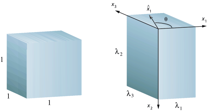
Figure 8: Interface wave propagation when the boundary $x_{2}=0$ is a principal plane of pre-strain. The $\hat{x}_{1}$ direction is the direction of propagation, making an angle $\theta$ with the principal direction of pre-strain $x_{1}$.

11 Governing equations

Hence we model this motion as

$$\{\boldsymbol{u},\dot{p},\boldsymbol{s}\}=\{\boldsymbol{U}(kx_{2}),\textrm{i}kP(kx_{2}),\textrm{i}k\boldsymbol{S}(kx_{2})\}\textrm{e}^{\textrm{i}k(c_{\theta}x_{1}+s_{\theta}x_{3}-vt)},$$ (103)

where $c_{\theta}=\cos\theta$, $s_{\theta}=\sin\theta$. By projecting the governing equations in the coordinate axis of the principal axes (where $\boldsymbol{\mathcal{A}_{0}}$ has 15 independent non-zero components, see Section 2), we can write them in the Stroh form (13) as a homogeneous linear system of six first-order differential equations, where $\boldsymbol{\xi}=[U_{1},U_{2},U_{3},S_{21},S_{22},S_{23}]^{t}$, see Destrade et al. (2005) for details. Here the matrices $-\boldsymbol{N}_{1}$, $\boldsymbol{N}_{2}$, $-\boldsymbol{N}_{3}$ are given by

$$\begin{bmatrix}0&c_{\theta}(\gamma_{21}-\sigma_{2})/\gamma_{21}&0\\ c_{\theta}&0&s_{\theta}\\ 0&s_{\theta}(\gamma_{23}-\sigma_{2})/\gamma_{23}&0\end{bmatrix},\quad\begin{bmatrix}1/\gamma_{21}&0&0\\ 0&0&0\\ 0&0&1/\gamma_{23}\end{bmatrix},\quad\begin{bmatrix}\chi&0&-\kappa\\ 0&\nu&0\\ -\kappa&0&\mu\end{bmatrix},$$ (104)

respectively, where

$$\chi=2c_{\theta}^{2}(\beta_{12}+\gamma_{21}-\sigma_{2})+s_{\theta}^{2}\gamma_{31},$$

$$\nu=c_{\theta}^{2}[\gamma_{12}-(\gamma_{21}-\sigma_{2})^{2}/\gamma_{21}]+s_{\theta}^{2}[\gamma_{32}-(\gamma_{23}-\sigma_{2})^{2}/\gamma_{23}],$$

$$\mu=c_{\theta}^{2}\gamma_{13}+2s_{\theta}^{2}(\beta_{23}+\gamma_{23}-\sigma_{2}),$$

$$\kappa=c_{\theta}s_{\theta}(\beta_{13}-\beta_{12}-\beta_{23}-\gamma_{21}-\gamma_{23}+2\sigma_{2}),$$ (105)

and the $\gamma_{ij}$, $\beta_{ij}$ are defined in (5).

Rogerson and Sandiford (1999) show that the propagation condition (16) is a cubic in $q^{2}$,

$$\gamma_{21}\gamma_{23}q^{6}-[(\gamma_{21}+\gamma_{23})X-c_{1}]\,q^{4}+(X^{2}-c_{2}X+c_{3})\,q^{2}+(X-c_{4})(X-c_{5})=0,$$ (106)

with $X=\rho v^{2}$ and

$$c_{1}=(\gamma_{21}\gamma_{13}+2\beta_{12}\gamma_{23})c_{\theta}^{2}+(\gamma_{23}\gamma_{31}+2\beta_{23}\gamma_{21})s_{\theta}^{2},$$

$$c_{2}=(\gamma_{23}+\gamma_{13}+2\beta_{12})c_{\theta}^{2}+(\gamma_{21}+\gamma_{31}+2\beta_{23})s_{\theta}^{2},$$

$$c_{3}=(\gamma_{12}\gamma_{23}+2\beta_{12}\gamma_{13})c_{\theta}^{4}+(\gamma_{21}\gamma_{32}+2\beta_{23}\gamma_{31})s_{\theta}^{4}$$

$$\phantom{123456}+[\gamma_{12}\gamma_{21}+\gamma_{13}\gamma_{31}+\gamma_{23}\gamma_{32}-(\beta_{13}-\beta_{12}-\beta_{23})^{2}+4\beta_{12}\beta_{23}]c_{\theta}^{2}s_{\theta}^{2},$$

$$c_{4}=\gamma_{12}c_{\theta}^{2}+\gamma_{32}s_{\theta}^{2},$$

$$c_{5}=\gamma_{13}c_{\theta}^{4}+2\beta_{13}c_{\theta}^{2}s_{\theta}^{2}+\gamma_{31}s_{\theta}^{4}.$$ (107)

12 Resolution for Rayleigh surface waves

Finding the eigenvectors $\boldsymbol{\zeta}^{1}$, $\boldsymbol{\zeta}^{2}$, $\boldsymbol{\zeta}^{3}$ of $\boldsymbol{N}$ corresponding to the qualifying roots $q_{1}$, $q_{2}$, $q_{3}$ (say) is a lengthy task by hand, best left to a computer algebra system. In the end, we find that the $\boldsymbol{\zeta}^{i}$ are of the forms:

$$\boldsymbol{\zeta}^{1}=\begin{bmatrix}\boldsymbol{a}^{1}\\ \boldsymbol{b}^{1}\end{bmatrix},\qquad\boldsymbol{\zeta}^{2}=\begin{bmatrix}\boldsymbol{a}^{2}\\ \boldsymbol{b}^{2}\end{bmatrix},\qquad\boldsymbol{\zeta}^{3}=\begin{bmatrix}\boldsymbol{a}^{3}\\ \boldsymbol{b}^{3}\end{bmatrix},$$ (108)

where

$$\boldsymbol{a}^{j}=\begin{bmatrix}a_{4}q_{i}^{4}+a_{2}q_{i}^{2}+a_{0}\\ -q_{j}^{5}+b_{3}q_{j}^{3}+b_{1}q_{j}\\ d_{4}q_{j}^{4}+d_{2}q_{j}^{2}+d_{0}\end{bmatrix},\qquad\boldsymbol{b}^{j}=\begin{bmatrix}h_{3}q_{j}^{3}+h_{1}q_{j}\\ (\nu-X)(q_{j}^{4}+mq_{j}^{2}+n)\\ g_{3}q_{j}^{3}+g_{1}q_{j}\end{bmatrix}.$$ (109)

Here the quantities $m$ and $n$ are given by

$$m=\left(\frac{1}{\gamma_{21}}+\frac{(\gamma_{21}-\sigma_{2})^{2}}{\gamma_{21}^{2}(\nu-X)}c_{\theta}^{2}\right)[\eta-X]+\left(\frac{1}{\gamma_{23}}+\frac{(\gamma_{23}-\sigma_{2})^{2}}{\gamma_{23}^{2}(\nu-X)}s_{\theta}^{2}\right)[\mu-X]\\ -2\kappa\frac{(\gamma_{21}-\sigma_{2})(\gamma_{23}-\sigma_{2})}{\gamma_{21}\gamma_{23}(\nu-X)}c_{\theta}s_{\theta},$$ (110)

$$n=\left\{1+\left[\frac{(\gamma_{21}-\sigma_{2})^{2}}{\gamma_{21}}c_{\theta}^{2}+\frac{(\gamma_{23}-\sigma_{2})^{2}}{\gamma_{23}}s_{\theta}^{2}\right](\nu-X)^{-1}\right\}\\ \times[(\mu-X)(\eta-X)-\kappa^{2}]/(\gamma_{21}\gamma_{23}).$$ (111)

The expressions for the quantities $a_{i}$, $b_{i}$, $d_{i}$, $h_{i}$, $g_{i}$ are too lengthy to reproduce but they are easily obtained in a formal manner using a computer algebra system; as it turns out, these constants are not needed in the secular equation for Rayleigh surface waves. Indeed, the expression for the surface impedance matrix $\boldsymbol{M}$ is very lengthy, but its determinant factorizes greatly. Hence we find that the exact secular equation for Rayleigh surface waves (22) reduces to (Taziev, 1987; Destrade et al., 2005)

$$n\omega_{\text{I}}-\omega_{\text{III}}(m-\omega_{\text{II}})=0,$$ (112)

where

$$\omega_{\text{I}}=-(q_{1}+q_{2}+q_{3}),\quad\omega_{\text{II}}=q_{1}q_{2}+q_{2}q_{3}+q_{3}q_{1},\quad\omega_{\text{III}}=-q_{1}q_{2}q_{3}.$$ (113)

This secular equation remains implicit as long as the roots $q_{1}$, $q_{2}$, $q_{3}$ satisfying the decay condition are not known. To compute them, we must find the wave speed, by using the fundamental equations (30).

First, using the explicit expression (104) of the Stroh matrix $\boldsymbol{N}$, we compute $\boldsymbol{N}^{-1}$ and $\boldsymbol{N}^{3}$, and in particular we find explicit expressions for the lower left blocks $\boldsymbol{K}^{(1)}=\boldsymbol{N}_{3}+\rho v^{2}\boldsymbol{I}$, $\boldsymbol{K}^{(-1)}$, $\boldsymbol{K}^{(3)}$. Next, we use the result (Destrade, 2005) that $\boldsymbol{U}(0)$ is in the form

$$\boldsymbol{U}(0)=U_{1}(0)[1,\textrm{i}\alpha,\beta]^{\text{T}},$$ (114)

where $\alpha$, $\beta$ are real numbers, to write the fundamental equations (30) at $n=-1,1,3$ as the following system of three equations,

$$\begin{bmatrix}K_{13}^{(-1)}&K_{33}^{(-1)}&K_{22}^{(-1)}\\ K_{13}^{(1)}&K_{33}^{(1)}&K_{22}^{(1)}\\ K_{13}^{(3)}&K_{33}^{(3)}&K_{22}^{(3)}\end{bmatrix}\begin{bmatrix}2\beta\\ \beta^{2}\\ \alpha^{2}\end{bmatrix}=\begin{bmatrix}-K_{11}^{(-1)}\\ -K_{11}^{(1)}\\ -K_{11}^{(3)}\end{bmatrix}.$$ (115)

Then, we solve this non-homogeneous system by Cramer’s rule to find

$$2\beta=\Delta_{1}/\Delta,\qquad\beta^{2}=\Delta_{2}/\Delta,$$ (116)

where $\Delta$, $\Delta_{1}$, and $\Delta_{2}$ are the following determinants,

$$\Delta=\begin{vmatrix}K_{13}^{(-1)}&K_{33}^{(-1)}&K_{22}^{(-1)}\\ K_{13}^{(1)}&K_{33}^{(1)}&K_{22}^{(1)}\\ K_{13}^{(3)}&K_{33}^{(3)}&K_{22}^{(3)}\end{vmatrix},\\ \Delta_{1}=\begin{vmatrix}-K_{11}^{(-1)}&K_{33}^{(-1)}&K_{22}^{(-1)}\\ -K_{11}^{(1)}&K_{33}^{(1)}&K_{22}^{(1)}\\ -K_{11}^{(3)}&K_{33}^{(3)}&K_{22}^{(3)}\end{vmatrix},\qquad\quad\;\\ \Delta_{2}=\begin{vmatrix}K_{13}^{(-1)}&-K_{11}^{(-1)}&K_{22}^{(-1)}\\ K_{13}^{(1)}&-K_{11}^{(1)}&K_{22}^{(1)}\\ K_{13}^{(3)}&-K_{11}^{(3)}&K_{22}^{(3)}\end{vmatrix}.$$ (117)

Finally we write down the compatibility of equations (116) as

$$\Delta_{1}^{2}-4\Delta\Delta_{2}=0,$$ (118)

which is the explicit secular equation for non-principal surface waves in deformed incompressible materials.

In general this equation is a polynomial of degree 12 in $\rho v^{2}$ (Taziev, 1989; Destrade et al., 2005), easy to solve numerically. Of the 12 possible roots, we keep those which are real, positive, and give a subsonic speed (that is a speed for which the bicubic (106) has three pairs of complex conjugate roots). We then test the remaining speeds against the exact secular equation (112).

13 Examples

neo-Hookean solid.

The neo-Hookean form of the strain energy density for an incompressible isotropic solid is a sub-case of the Mooney-Rivlin form, namely $\mathcal{D}_{2}=0$ in (52) so that

$$W=\mathcal{D}_{1}(\lambda_{1}^{2}+\lambda_{2}^{2}+\lambda_{3}^{2})/2.$$ (119)

It leads to a stress-strain relationship (5) which is “linear” with respect to the left Cauchy-green strain tensor,

$$\boldsymbol{\sigma}=-p\boldsymbol{I}+\mathcal{D}_{1}\boldsymbol{B}.$$ (120)

The neo-Hookean model is unable to capture neither qualitatively nor quantitatively experimental data, over any range of deformations (Saccomandi, 2004). It is nonetheless a highly popular model in the literature because it forms the basis of a statistical treatment for the molecular description of rubber elasticity (Treloar, 1949).

With respect to wave propagation, it has more peculiar properties than the Mooney-Rivlin material, because here,

$$\gamma_{ij}=\mathcal{D}_{1}\lambda_{i}^{2},\qquad 2\beta_{ij}=\mathcal{D}_{1}(\lambda_{i}^{2}+\lambda_{j}^{2}),$$ (121)

which leads to great simplifications in the matrices $\boldsymbol{N}_{1}$, $\boldsymbol{N}_{2}$, $\boldsymbol{N}_{3}$ of (104).

Now placing ourselves in the coordinates system ($\hat{x}_{1},x_{2},\hat{x}_{3}$) attached to the wave propagation, see Figure 8, we introduce the functions $\hat{U}_{i}$, $\hat{S}_{2i}$ ($i=1,2,3$), defined by

$$\hat{U}_{i}=\Omega_{ij}U_{j},\quad\hat{S}_{2i}=\Omega_{ij}S_{2j},\quad\text{where}\quad\Omega_{ij}=\begin{bmatrix}c_{\theta}&0&-s_{\theta}\\ 0&1&0\\ s_{\theta}&0&c_{\theta}\end{bmatrix}.$$ (122)

With these functions, the governing equations (13) decouple the anti-saggital motion $[\hat{U}_{3},\hat{S}_{23}]$ from its saggital counterpart (recall that the direction of propagation and the normal to the interface define what is called the saggital plane.) For the latter motion we find

$$[\hat{U}_{1}^{\prime},\hat{U}_{2}^{\prime},\hat{S}_{21}^{\prime},\hat{S}_{22}^{\prime}]^{t}=\textrm{i}\boldsymbol{N}[\hat{U}_{1},\hat{U}_{2},\hat{S}_{21},\hat{S}_{22}]^{t},$$ (123)

with

$$\boldsymbol{N}=\begin{bmatrix}0\ &\ -1+\overline{\sigma}_{2}\ &\ 1/(\mathcal{D}_{1}\lambda_{2}^{2})&0\\ -1\ &\ 0\ &\ 0&0\\ \rho v^{2}-\hat{\chi}\ &\ 0\ &\ 0&-1\\ 0\ &\ \rho v^{2}-\hat{\nu}\ &\ -1+\overline{\sigma}_{2}\ &0\end{bmatrix},$$ (124)

where

$$\hat{\chi}=\mathcal{D}_{1}(c_{\theta}^{2}\lambda_{1}^{2}+s_{\theta}^{2}\lambda_{3}^{2}+3\lambda_{2}^{2}-2\overline{\sigma}_{2}),\quad\hat{\nu}=\mathcal{D}_{1}[c_{\theta}^{2}\lambda_{1}^{2}+s_{\theta}^{2}\lambda_{3}^{2}+\lambda_{2}^{2}(1-\overline{\sigma}_{2})^{2}],$$ (125)

and $\overline{\sigma}_{2}=\sigma_{2}/(\mathcal{D}_{1}\lambda_{2}^{2})$ is a non-dimensional measure of the pre-stress. The associated propagation condition is

$$(q^{2}+1)[\lambda_{2}^{2}q^{2}+(c_{\theta}^{2}\lambda_{1}^{2}+s_{\theta}^{2}\lambda_{3}^{2})-\rho v^{2}/\mathcal{D}_{1}]=0.$$ (126)

In other words, the situation is formally the same as that for principal waves in Mooney-Rivlin material, see Section 7. The conclusion is that the speed is given by

$$\rho v^{2}=\mathcal{D}_{1}(c_{\theta}^{2}\lambda_{1}^{2}+s_{\theta}^{2}\lambda_{3}^{2}-\lambda_{2}^{2}\eta^{2}),$$ (127)

where $\eta$ is the real root of (56). Flavin (1963) established this result at $\sigma_{2}=0$. As he also showed, the situation gets more complicated for Mooney-Rivlin solids, because the wave is no longer plane polarized for a triaxial pre-stretch.

Mooney-Rivlin solid.

The Mooney-Rivlin strain energy density (52) at $\mathcal{D}_{2}\neq 0$ does not lead to a decoupling of the saggital motion from the anti-saggital motion. However, as in Sections 3 and 4, we find that the propagation condition factorizes, here as

$$(q^{2}+1)(q^{4}-Sq^{2}+P)=0,$$ (128)

where

$$S=\left(\frac{1}{\gamma_{21}}+\frac{1}{\gamma_{23}}\right)X-\left(\frac{\gamma_{12}}{\gamma_{21}}+\frac{\gamma_{13}}{\gamma_{23}}\right)c_{\theta}^{2}-\left(\frac{\gamma_{31}}{\gamma_{21}}+\frac{\gamma_{32}}{\gamma_{23}}\right)s_{\theta}^{2},$$

$$P=(X-\gamma_{12}c_{\theta}^{2}-\gamma_{32}s_{\theta}^{2})(X-\gamma_{13}c_{\theta}^{2}-\gamma_{31}s_{\theta}^{2})/(\gamma_{21}\gamma_{23}).$$ (129)

Flavin (1963) was the first to notice that $q_{1}=\textrm{i}$ is an attenuation factor for non-principal waves in Mooney-Rivlin solids. Pichugin (2001) showed that a necessary and sufficient condition for the factorization (128) to occur is that the relations (54) hold; he also showed, completing earlier work by Willson (1973a), that another factorization of the general bicubic (106) also occurs, this time for any strain energy function, when two of the principal stretches of pre-strain are equal (equi-biaxial pre-strain). Finally note that $(q^{2}+1)$ always comes out as a factor in the propagation condition for inhomogeneous waves in Mooney-Rivlin solids, whatever the direction of propagation is (not necessarily in a principal plane as here), see Destrade (2002) for details.

Thanks to the factorization (128), we can actually compute explicitly the quantities $\omega_{\text{I}}$, $\omega_{\text{II}}$, $\omega_{\text{III}}$ of (113). Indeed, we now have

$$q_{1}=\textrm{i},\qquad q_{2}q_{3}=-\sqrt{P},\qquad q_{2}+q_{3}=\textrm{i}\sqrt{2\sqrt{P}-S},$$ (130)

so that

$$\omega_{\text{I}}=-\textrm{i}(1+\sqrt{2\sqrt{P}-S}),\qquad-\omega_{\text{II}}=\sqrt{P}+\sqrt{2\sqrt{P}-S},\qquad\omega_{\text{III}}=\textrm{i}\sqrt{P},$$ (131)

leading to an explicit and exact form of the secular equation (112),

$$n\Bigl{(}1+\sqrt{2\sqrt{P}-S}\Bigr{)}+\sqrt{P}\Bigl{(}m+\sqrt{P}+\sqrt{2\sqrt{P}-S}\Bigr{)}=0.$$ (132)

This result allows us to investigate the influence of pre-stress on surface wave propagation (see Destrade et al. (2005) for an example) and to address an important question in the study of surface stability: how much can a Mooney-Rivlin half-space be compressed before it buckles? In Section 3 we found the critical stretch in a principal direction ($x_{1}$), indicating the appearance of wrinkles parallel to $x_{3}$, see Figure 2 for a visualization. However, could it be that wrinkles appeared earlier in the compression, in another direction? To answer this we take $X(=\rho v^{2})=0$ (onset of instability) and solve (132) for $\lambda$, for each value of $\theta$.

For instance, take the case of the following plane pre-strain,

$$\lambda_{1}=\lambda,\qquad\lambda_{2}=\lambda^{-1},\qquad\lambda_{3}=1,$$ (133)

imposed on a half-space made of the Mooney-Rivlin solid with material parameters

$$\mathcal{D}_{1}=2.0\mu,\qquad\mathcal{D}_{2}=0.8\mu,$$ (134)

where $\mu$ has the dimension of a stiffness (the shear modulus of this Mooney-Rivlin solid is $(\mathcal{D}_{1}+\mathcal{D}_{2})/2=1.4\mu$). Figure 9 displays the values of the critical stretch ratio, measured in the principal direction $x_{1}$, for each angle $\theta$ and for several values of the pre-stress $\sigma_{2}$. The solid line corresponds to $\sigma_{2}=0$. At $\theta=0$ we find the critical compression ratio $\lambda_{\text{c}}^{0}$ (say) for wrinkles aligned along $x_{3}$; hence the solid curve starts at $\lambda_{\text{c}}^{0}=0.544$ as expected from solving (57) with $v=0$ and $\lambda_{1}=\lambda_{\text{c}}^{0}=\lambda_{2}^{-1}$. At $\theta\neq 0$ we find that the critical compression stretch is below $\lambda_{\text{c}}^{0}$; it follows that $\lambda_{\text{c}}^{0}$ is the absolute critical stretch of compression for our example (133), (134). Of course, for Mooney-Rivlin solids other than (134), or for pre-strains other than (133), or for solids other than Mooney-Rivlin solids, we might end up with a different behaviour in compression. However the same analysis can be brought in each case to its conclusion, with no additional difficulty.

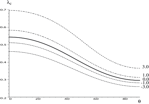
Figure 9: Critical stretch ratio of compression for a Mooney-Rivlin material as a function of the angle between the normal to the wrinkles and the principal axis of greatest compression. The Mooney-Rivlin solid is subject to a finite plane strain compression ($\lambda_{3}=1$); its material parameters are $\mathcal{D}_{1}=2.0\mu$, $\mathcal{D}_{2}=0.8\mu$; the pre-stress normal to the boundary is given by $\sigma_{2}/\mu=$ -3.0, -1.0, 0.0, 1.0, 3.0 ($\mu$ has the dimension of a stiffness).

Gent solid.

We find that the elastic moduli (5) for Gent materials (100) are given in general by

$$\gamma_{ij}=C\dfrac{J_{m}}{J_{m}+3-\lambda_{1}^{2}-\lambda_{2}^{2}-\lambda_{3}^{2}}\lambda_{i}^{2},$$

$$2\beta_{ij}=C\dfrac{J_{m}}{J_{m}+3-\lambda_{1}^{2}-\lambda_{2}^{2}-\lambda_{3}^{2}}\left[\lambda_{i}^{2}+\lambda_{j}^{2}+\dfrac{2(\lambda_{i}^{2}-\lambda_{j}^{2})^{2}}{J_{m}+3-\lambda_{1}^{2}-\lambda_{2}^{2}-\lambda_{3}^{2}}\right].$$ (135)

Now consider that a half-space made of a Gent material with $J_{m}=9.0$ is subject to a large shear such that the boundary is the plane of shear (in Section 4, the boundary was the glide plane) and the boundary $x_{2}=0$ is free of tractions. Then the principal stretches are

$$\lambda_{1}=\sqrt{1+K^{2}/4}+K/2,\qquad\lambda_{2}=1,\qquad\lambda_{3}=\sqrt{1+K^{2}/4}-K/2,$$ (136)

and of course, $\lambda_{1}^{2}+\lambda_{2}^{2}+\lambda_{3}^{2}-3=K^{2}$.

Figure 10 shows the variations of the surface wave speed in the plane of shear, with respect to the angle between the direction of propagation ($\hat{x}_{1}$) and the direction of shear ($X_{1}$). For a shear of amount $K=0.5$, the principal axis of greatest stretch $x_{1}$ makes an angle $37.9^{\circ}$ with the direction of shear, and the principal axis of smallest stretch $x_{3}$ makes an angle $127.9^{\circ}$ with the direction of shear. For $K=1$, those two angles are $31.7^{\circ}$ and $121.7^{\circ}$ , respectively; for $K=2$, those two angles are $22.5^{\circ}$ and $112.5^{\circ}$ , respectively. Clearly, the surface wave reaches extremal values along those directions, indicating that the principal directions can be determined acoustically.

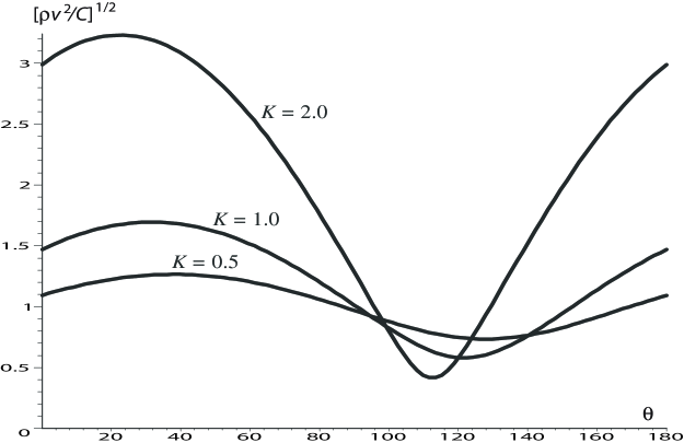
Figure 10: Wave propagating in the plane of shear of a semi-infinite sheared Gent solid with $J_{m}=9.0$: scaled speed $\sqrt{\rho v^{2}/C}$ as a function of the angle between the propagation direction and the direction of shear, for several values of the amount of shear.

Chapter 6 Concluding remarks

This Chapter has presented several situations where it is possible to derive explicit secular equations in exact form and in polynomial form, for incremental waves propagating along the plane interface of one (or two) deformed semi-infinite hyperelastic solid (rigidly bonded solids). The subject of interface waves in general is broad and includes many other situations and geometries such as, to name but a few: the addition of a layer of finite thickness (Love waves, Lamb waves, etc.), or of a fluid (Scholte waves for inviscid fluids, Stoneley waves for viscous fluids, etc.), the consideration of an anisotropy due to families of extensible fibres, of cylindrical or spherical coordinates, or of curved boundaries, and so on. Reading the works by Ogden (2003, 2004) and by Guz (2002) and the references therein gives a good overview of the vast panorama spanned by these other types of interface wave problems.

This concluding Section expands on the reasons put forth to explain why it can be advantageous at times to seek explicit secular equations rather than to turn to numerics outright. Among other things, explicit secular equations in polynomial form

• are easy to solve numerically, with the greatest precision required;

• are sometimes surprisingly simple and short, in spite of a complicated or even unsolvable propagation condition;

• lend themselves to simple asymptotic treatments, leading to approximate analytical expressions for the wave speed;

• account for all the solutions satisfying the propagation condition and the boundary condition at the interface.

14 Numerics

Point (i) goes without saying because the numerical methods used to determine the roots of a polynomial are safe and robust. Of course, at most only one root corresponds to the actual solution and all the other roots must be discarded as being spurious. So, once a likely root is found numerically (that is a root $\rho v^{2}$ which is real and positive), it must be checked that at that speed the exact secular equation is satisfied. This routine check is simple enough to perform (solve the propagation condition, find the corresponding impedance matrix, check that (22) (for Rayleigh waves) or that (23) (for Stoneley waves) is satisfied).

Other numerical techniques to find the interface wave speed invoke the Barnett-Lothe-Stroh integral formalism (see Ting (1996) for an account), computational algorithms for eigenvalue problems Taylor (1981), or an algebraic Ricatti equation for the impedance matrix (see the Chapter by Fu in this book and the references therein) to determine $M(v)$ for any numerical value of $v$; then $v$ is varied in order to satisfy the exact secular equation up to the desired precision. This however is not always an easy task, as seen in the following example.

Consider the Mooney-Rivlin solid with material parameters (134), maintained in a state of static pre-strain, with (Rogerson and Sandiford, 1999),

$$\lambda_{1}=\sqrt{3.695},\qquad\lambda_{2}=\sqrt{0.7},\qquad\lambda_{3}=(\lambda_{1}\lambda_{2})^{-1},\qquad\sigma_{2}=0.8\mu.$$ (137)

Take the interface between the solid and the vacuum to be the principal plane $x_{2}=0$ and study the propagation of a Rayleigh surface wave in a direction close to $x_{3}$ ($\theta$ is close to $90^{\circ}$ in Figure 8.)

Along $x_{3}$ we have a principal wave, travelling with a speed $v(90)$ say, found from Section 6. Here (Destrade et al., 2005) we find that $v(90)\simeq 1.327\sqrt{\mu/\rho}$. On the other hand, a shear (homogeneous) bulk wave linearly polarized along $x_{1}$ travels with speed $v_{1}$ say, given by $\rho v_{1}^{2}=\gamma_{31}$, and a shear (homogeneous) bulk wave linearly polarized along $x_{2}$ travels with speed $v_{2}$ say, given by $\rho v_{2}^{2}=\gamma_{32}$. Here we find that $v_{1}\simeq 1.384\sqrt{\mu/\rho}$ and that $v_{2}\simeq 0.995\sqrt{\mu/\rho}$, showing that the surface wave travels with a speed which is intermediate between those of the shear bulk waves. That principal wave is two-partial and polarized in the ($x_{2}x_{3}$) plane, which is why it can afford to be faster than the shear bulk wave polarized in the $x_{1}$ direction. Also, it is isolated, in the sense that the transition toward a surface wave propagating in a direction $\theta\neq 90^{\circ}$ is abrupt, because this latter wave is tri-partial and must therefore travel with a speed $v(\theta)$ say, which is less than the speed of any homogeneous bulk shear wave, in particular less than $\sqrt{c_{4}/\rho}$ and less than $\sqrt{c_{5}/\rho}$, where $c_{4}$ and $c_{5}$ are defined in (11). Figure 11 shows the variations of these 3 speeds in the neighbourhood of the $x_{3}$ axis and makes those features clear.

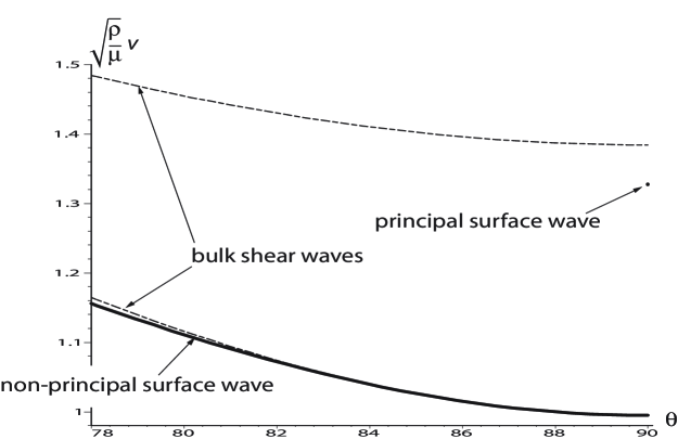
Figure 11: Wave propagation in the $x_{2}$ principal plane of semi-infinite Mooney-Rivlin solid (134) deformed by (137): variations of scaled speed $\sqrt{\rho v^{2}/\mu}$ as a function of the angle, near the $x_{3}$ direction.

Now if our numerical method for the surface wave speed relies on using the known principal wave speed as an “initial guess”, then it might run into difficulties here because of the isolation of the principal wave. This special feature is characteristic of strongly anisotropic crystals in linear elasticity. In incremental dynamics, it can occur at will, simply by deforming the solid sufficiently to create a strong strain-induced anisotropy.

Also, as is clear from the Figure, the surface wave travels with a speed which is extremely close to that of the bulk shear wave $\sqrt{c_{4}/\rho}$. Hence at $\theta=89.99^{\circ}$, the speed of the former is given by

$$\sqrt{\rho v^{2}/\mu}=0.9948641879596778\ldots,$$ (138)

whilst the speed of the latter is given by

$$\sqrt{c_{4}/\mu}=0.9948641879596860\ldots.$$ (139)

Consequently, if a numerical scheme for the surface wave speed relies on increasing $v$ in small steps until $\text{det }M(v)=0$ is satisfied to any desired precision, then it will have to be pushed to the 14th significant digit to insure that the speed does not correspond to a bulk wave! Here the explicit polynomial secular gives only two positive roots, and it is a routine check to verify that only (138) satisfies the exact secular equation.

15 Polynomials

For an interface wave propagating in any direction in a deformed solid, the propagation condition is a sextic in general. Such is for instance the case for a wave propagating in any direction in the glide plane of the sheared block in Figure 4. Although a sextic is unsolvable analytically, it is nonetheless possible to find a polynomial secular equation for a Rayleigh surface wave, see Taziev (1989) or Ting (2004) for details. The polynomial turns out to be of degree 27 in $\rho v^{2}$. For Stoneley interface waves it does not seem practical to look for a polynomial secular equation.

For an interface wave propagating in any direction in a principal plane of pre-deformation, the propagation condition is the bicubic (106). Although formulas exist for the roots of a cubic, the analytical resolution of (106) proves to be complicated because it is not known a priori whether the roots are purely imaginary or have a non-zero real part and accordingly, which formula should be used. However, the polynomial explicit secular equation for a Rayleigh surface wave is of degree 12 in $\rho v^{2}$ as seen earlier. This is also the case in the symmetry plane of an orthorhombic or monoclinic crystal. In the symmetry plane of a cubic crystal, the degree of the polynomial comes down to 10, as noted by Taylor (1981). For a two-partial surface wave, coupled to electrical fields through piezoelectricity in 2mm crystals, the polynomial is also of degree 10 in $\rho v^{2}$ for metallized boundary conditions (there the propagation condition is also a bicubic, see Collet and Destrade (2005)).

For a two-partial (non-principal) interface wave polarized in a principal plane of pre-deformation, the propagation condition is a quartic,

$$q^{4}+d_{3}q^{3}+d_{2}q^{2}+d_{1}q+d_{0}=0,$$ (140)

say (see (78) for the case of simple shear). In contrast to the case of the bicubic above, we know here what the form of the roots should be, because the roots of a quartic are either two pairs of complex conjugate numbers, or one double real root with one pair of complex conjugate numbers, or four real roots. Here only the first scenario is acceptable in order to satisfy the decay condition (17) and thus a single formula, always valid, is required; it can be found in the textbooks. First introduce in turn the quantities $r$, $s$, and $h$, defined by

$$r=d_{2}-\textstyle{\frac{3}{8}}d_{3}^{2},\quad s=d_{1}-\textstyle{\frac{1}{2}}d_{2}d_{3}+\textstyle{\frac{1}{8}}d_{3}^{2},\quad h=d_{0}-\textstyle{\frac{1}{4}}d_{1}d_{3}+\textstyle{\frac{1}{16}}d_{2}d_{3}^{2}-\textstyle{\frac{3}{256}}d_{3}^{4},$$ (141)

the quantities $\lambda$ and $\phi\in]0,\pi/3]$, defined by

$$\lambda=\textstyle{\frac{1}{27}}\left(12h+r^{2}\right)^{3/2},\qquad\phi=\textstyle{\frac{1}{3}}\arccos\left[\frac{1}{2\lambda}\left(\textstyle{\frac{2}{27}}r^{3}+s^{2}-\textstyle{\frac{8}{3}}rh\right)\right],$$ (142)

and the quantities $z_{1}$, $z_{2}$, and $z_{3}$, defined by

$$z_{1}=2\lambda^{1/3}\cos(\phi)-\textstyle{\frac{2}{3}}r,$$

$$z_{2}=2\lambda^{1/3}\cos(\phi+2\pi/3)-\textstyle{\frac{2}{3}}r,$$

$$z_{3}=2\lambda^{1/3}\cos(\phi+4\pi/3)-\textstyle{\frac{2}{3}}r.$$ (143)

Then the qualifying roots are

$$p_{1}=\textstyle{\frac{1}{2}}\text{sign}(s)\sqrt{z_{1}}-\textstyle{\frac{1}{4}}d_{3}+\textstyle{\frac{1}{2}}\textrm{i}(\sqrt{-z_{2}}+\sqrt{-z_{3}}),$$

$$p_{2}=-\textstyle{\frac{1}{2}}\text{sign}(s)\sqrt{z_{1}}-\textstyle{\frac{1}{4}}d_{3}+\textstyle{\frac{1}{2}}\textrm{i}(\sqrt{-z_{2}}-\sqrt{-z_{3}}),$$ (144)

where $\text{sign}(s)$ equals 1 if $s$ is non-negative and $-1$ otherwise. These formulas are perfectly well handled by a computer algebra system, so that $M$, and ultimately the exact secular equation, can be found. It then means that any interface wave problem can be solved exactly. Nonetheless it might still be rewarding to look for the polynomial secular equation, to check whether they turn out to be simple. For instance, the polynomial secular equation for Rayleigh waves is a quartic in the squared speed when the solid is sheared (Section 9), or tri-axially stretched and then sheared (Destrade and Ogden, 2005), or when the wave is polarized in the symmetry plane of a crystal (Currie, 1979). Now consider a flexural wave travelling along the free edge of a thin (Love-Kirchhoff) orthotropic plate where the edge makes an arbitrary angle with a principal axis of symmetry. Thompson et al. (2002) show that the corresponding propagation condition is a quartic, but turn to a numerical resolution. However Fu (2003) shows that the polynomial secular equation is just a cubic in the squared speed. Finally consider the case of a piezoacoustic Bleustein-Gulyaev surface wave in a rotated $Y$-cut about the $Z$ axis for $\overline{4}$ crystals. There also the propagation condition is a quartic, but the fundamental equations reveal that the polynomial secular equation for metallized boundary conditions is simply a quadratic in the squared speed (Collet and Destrade, 2004). Clearly it is a worthy enterprise to unearth these polynomials rather than use numerics or the formulas (141)-(15).

16 Approximate expressions

Once the polynomial secular equation is established, in the form $\mathcal{P}(v)=0$, say, it is a straightforward matter to derive an analytical approximation for $v$. Calling $v_{0}$ an initial approximation, we find in the first order that

$$v\simeq v_{0}-\mathcal{P}(v_{0})/\mathcal{P}^{\prime}(v_{0}).$$ (145)

Of course we must choose $v_{0}$ judiciously for an optimal expression.

Here we work out a simple example. We take a solid half-space subject to a hydrostatic pressure only, so that $\lambda_{1}=\lambda_{2}=\lambda_{3}\equiv\lambda$ say, and $\sigma_{1}=\sigma_{2}=\sigma_{3}\equiv\sigma$ say. From the incompressibility constraint (1), $\lambda=1$ follows and we have a pre-stressed, but unstrained, solid. It is thus isotropic and a surface wave propagates with the same speed in every direction. To derive the secular equation, we specialize for instance (50) to the isotropic case. We find that $\gamma_{12}=\gamma_{21}=\beta_{12}=\mu_{0}$, the infinitesimal shear modulus, and the exact secular equation is (Dowaikh and Ogden, 1990)

$$f(\eta)=\eta^{3}+\eta^{2}+(3-2\overline{\sigma})\eta-(1-\overline{\sigma})^{2}=0,$$ (146)

where $\overline{\sigma}\equiv\sigma/\mu_{0}$ and $\eta=\sqrt{1-\rho v^{2}/\mu_{0}}$. Calling $c\equiv\sqrt{\rho v^{2}/\mu_{0}}$ a dimensionless measure of the wave speed, and multiplying (146) by $f(-\eta)$, gives the polynomial secular equation (Dowaikh and Ogden, 1990),

$$\mathcal{P}(v)\equiv c^{6}-4(2-\overline{\sigma})c^{4}+6(\overline{\sigma}-2)^{2}c^{2}+(\overline{\sigma}^{2}-4)(\overline{\sigma}-2)^{2}=0.$$ (147)

In the region where $c$ is close to 1, the first order approximation (145) gives $c\simeq 1-\mathcal{P}(1)/\mathcal{P}^{\prime}(1)$, that is

$$c\simeq\dfrac{21-28\overline{\sigma}+6\overline{\sigma}^{2}+4\overline{\sigma}^{3}-\overline{\sigma}^{4}}{22-32\overline{\sigma}+12\overline{\sigma}^{2}}.$$ (148)

In particular we find that for an unstressed incompressible solid, $c\simeq 21/22=0.9545\ldots$, which is a good approximation to the value found from the exact equation 0.9553…(Lord Rayleigh, 1885). On Figure 12 we superpose the approximate and exact curves, and find good agreement in the $\overline{\sigma}=-1$ to $\overline{\sigma}=1$ region. Beyond that range, $c$ departs from the neighbourhood of 1, and a better choice must be made for the initial guess. This point is not developed further here but it is clearly exposed in the paper by Mozhaev (1991).

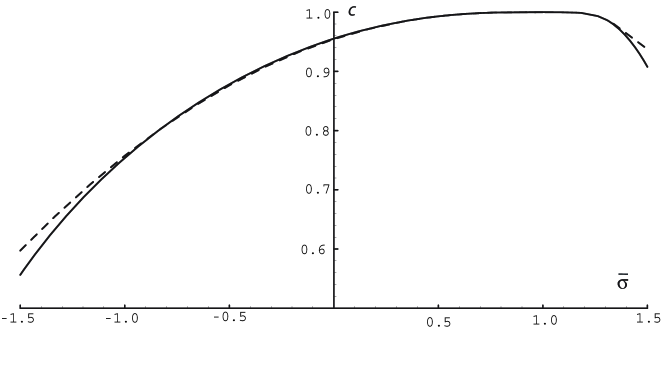
Figure 12: Surface wave speed in an incompressible solid subject to hydrostatic pressure only. Solid plot: exact calculation, dashed plot: approximate calculation.

17 Other waves

Taylor (1981) and Taziev (1989) both remarked that many of the roots to an explicit secular equation in polynomial form have a physical origin, because they correspond to a motion satisfying both the equations of motion and the boundary conditions at the interface. In particular for the solid/vacuum interface, the polynomial provides the parameters not only for the Rayleigh surface wave, but also for pseudo-surface waves, for Brewster reflection of bulk waves, for the reflection of inhomogeneous waves, for “organ-pipe” modes, etc.

One of the most important root is that corresponding to a leaky surface wave (if it exists), whose energy is diffused slowly into the half-space, and for which the classical methods evoked in Section 14 run into major difficulties.

Another application for this wealth of information is that many more wavefronts can be found, in particular those observed in the neighbourhood of cusps, which correspond to the interference of inhomogeneous plane waves (Huet, 2006). Figure 13 shows the remarkable correspondence obtained between experiment and predictions, for wavefronts propagating on the surface of a copper sample (cubic symmetry). Here the explicit secular equation proves useful because it is easy to differentiate, as required for the derivation of the curve.

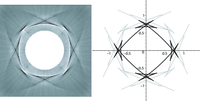
Figure 13: Wavefronts on the surface of copper cut along a symmetry plane. Left: experimental results obtained by LASER impact (Huet, 2006). Right: predictions derived from the secular equation in polynomial form, showing in black, the Rayleigh wave wavefront and in grey, the wavefronts due to leaky waves and interference of inhomogeneous waves.

References

- Barnett (2000) D.M. Barnett. Bulk, surface, and interfacial waves in anisotropic linear elastic solids. International Journal of Solids and Structures, 37:45–54, 2000.
- Barnett and Lothe (1985) D.M. Barnett and J. Lothe. Free surface (Rayleigh) waves in anisotropic elastic half-spaces: the surface impedance method. Proceedings of the Royal Society of London, Series A, 402:135–152, 1985.
- Biot (1963) M.A. Biot. Surface instability of rubber in compression. Applied Science Research, Series A, 12:168–182, 1963.
- Boulanger and Hayes (1992) Ph. Boulanger and M. Hayes. Finite-amplitude waves in deformed Mooney-Rivlin material. Quarterly Journal of Mechanics and Applied Mathematics, 45:575–593, 1992.
- Chadwick (1976) P. Chadwick. Continuum Mechanics. Allen & Unwin, 1976.
- Chadwick (1995) P. Chadwick. Interfacial and surface waves in pre-strained isotropic elastic media. ZAMP, 46:S51–S71, 1995.
- Chadwick (1997) P. Chadwick. The application of the Stroh formalism to prestressed elastic media. Mathematics and Mechanics of Solids, 2:379–403, 1997.
- Chadwick and Jarvis (1979a) P. Chadwick and D.A. Jarvis. Surface waves in a pre-stressed elastic body. Proceedings of the Royal Society of London, Series A, 366:517–536, 1979a.
- Chadwick and Jarvis (1979b) P. Chadwick and D.A. Jarvis. Interfacial waves in a pre-strained neo-Hookean body. Quarterly Journal of Mechanics and Applied Mathematics, 32:387–399, 1979b.
- Collet and Destrade (2004) B. Collet and M. Destrade. Explicit secular equations for piezoacoustic surface waves: Shear-horizontal modes. Journal of the Acoustical Society of America, 116:3432–3442, 2004.
- Collet and Destrade (2005) B. Collet and M. Destrade. Explicit secular equations for piezoacoustic surface waves: Rayleigh modes. Journal of Applied Physics, 98:054903, 2005.
- Connor and Ogden (1995) P. Connor and R.W. Ogden. The effect of shear on the propagation of elastic surface waves. International Journal of Engineering Science, 33:3432–3442, 1995.
- Connor and Ogden (1996) P. Connor and R.W. Ogden. The influence of shear strain and hydrostatic stress on stability and elastic waves in a layer. International Journal of Engineering Science, 34:375–397, 1996.
- Currie (1979) P.K. Currie. The secular equation for Rayleigh waves on elastic crystals. Quarterly Journal of Mechanics and Applied Mathematics, 32:163–173, 1979.
- Destrade (2000) M. Destrade. Finite-amplitude inhomogeneous plane waves in a deformed Mooney-Rivlin material. Quarterly Journal of Mechanics and Applied Mathematics, 53:343–361, 2000.
- Destrade (2002) M. Destrade. Small-amplitude inhomogeneous plane waves in a deformed Mooney-Rivlin material. Quarterly Journal of Mechanics and Applied Mathematics, 55:109–126, 2002.
- Destrade (2003) M. Destrade. Elastic interface acoustic waves in twinned crystals. International Journal of Solids and Structures, 40:7375–7383, 2003.
- Destrade (2005) M. Destrade. On interface waves in misoriented pre-stressed incompressible elastic solids. IMA Journal of Applied Mathematics, 70:3–14, 2005.
- Destrade and Fu (2006) M. Destrade and Y.B. Fu. The speed of interfacial waves polarized in a symmetry plane. International Journal of Engineering Science, 44:26–36, 2006.
- Destrade and Ogden (2005) M. Destrade and R.W. Ogden. Surface waves in a stretched and sheared incompressible elastic material. International Journal of Non Linear Mechanics, 40:241–253, 2005.
- Destrade et al. (2005) M. Destrade, M. Otténio, A.V. Pichugin, and G.A. Rogerson. Non-principal surface waves in deformed incompressible materials. International Journal of Engineering Science, 43:1092–1106, 2005.
- Dowaikh and Ogden (1990) M.A. Dowaikh and R.W. Ogden. On surface waves and deformations in a pre-stressed incompressible elastic solid. IMA Journal of Applied Mathematics, 44:261–284, 1990.
- Dowaikh and Ogden (1991) M.A. Dowaikh and R.W. Ogden. Interfacial waves and deformations in pre-stressed elastic media. Proceedings of the Royal Society of London, Series A, 433:313–328, 1991.
- Flavin (1963) J.N. Flavin. Surface waves in pre-stressed Mooney material. Quarterly Journal of Mechanics and Applied Mathematics, 16:441–449, 1963.
- Fu (2003) Y.B. Fu. Existence and uniqueness of edge waves in a generally anisotropic elastic plate. Quarterly Journal of Mechanics and Applied Mathematics, 56:605–616, 2003.
- Fu (2005a) Y.B. Fu. An explicit expression for the surface-impedance matrix of a generally anisotropic incompressible elastic material in a state of plane strain. International Journal of Non Linear Mechanics, 40:229–239, 2005a.
- Fu (2005b) Y.B. Fu. An integral representation of the surface-impedance tensor for incompressible elastic materials. Journal of Elasticity, 81:75–90, 2005b.
- Fu and Brookes (2006) Y.B. Fu and D.W. Brookes. An explicit expression for the surface-impedance tensor of a compressible monoclinic material in a state of plane strain. IMA Journal of Applied Mathematics, 71:434–445, 2006.
- Fu and Mielke (2002) Y.B. Fu and A. Mielke. A new identity for the surface impedance matrix and its application to the determination of surface-wave speeds. Proceedings of the Royal Society of London, Series A, 458:2523–2543, 2002.
- Gent (1996) A.N. Gent. A new constitutive relation for rubber. Rubber Chemistry and Technology, 69:59–61, 1996.
- Guz (2002) A.N. Guz. Elastic waves in bodies with initial (residual) stresses. International Applied Mechanics, 38:23–59, 2002.
- Hayes and Rivlin (1961) M.A. Hayes and R.S. Rivlin. Surface waves in deformed elastic materials. Archives for Rational Mechanics and Analysis, 8:358–380, 1961.
- Horgan and Saccomandi (2003) C.O. Horgan and G. Saccomandi. A description of arterial wall mechanics using limiting chain extensibility constitutive models. Biomechanics Modeling in Mechanobiology, 1:251–266, 2003.
- Huet (2006) G. Huet. Fronts d’Ondes Ultrasonores à la Surface d’un Milieu Semi-Infini Anisotrope: Théorie des Rayons Réels et Complexes. PhD Thesis, Université de Bordeaux 1, 2006.
- Hussain and Ogden (2000) W. Hussain and R.W. Ogden. Reflection and transmission of plane waves at a shear-twin interface. International Journal of Engineering Science, 38:1789–1810, 2000.
- Ingebrigsten and Tonning (1969) K.A. Ingebrigsten and A. Tonning. Elastic surface waves in crystals. Physical Review, 184:942–951, 1969.
- Karduna et al. (1997) A.R. Karduna, H.R. Halerpin, and F.C.P. Yin. Experimental and numerical analyses of indentation in finite-sized isotropic and anisotropic rubber-like materials. Annals of Biomedical Engineering, 25:1009–1016, 1997.
- Merodio and Ogden (2002) J. Merodio and R.W. Ogden. Material instabilities in fiber-reinforced nonlinearly elastic solids under plane deformation. Archives of Mechanics, 54:525–552, 2002.
- Mozhaev (1991) V.G. Mozhaev. Approximate analytical expressions for the velocity of Rayleigh waves in isotropic media and on the basal plane in high-symmetry crystals. Soviet Physics Acoustics, 37:1009–1016, 1991.
- Mozhaev (1995) V.G. Mozhaev. Some new ideas in the theory of surface acoustic waves in anisotropic media. In D.F. Parker and A.H. England, editors, IUTAM Symposium on Anisotropy, Inhomogeneity and Nonlinearity in Solid Mechanics, pages 455–462. Kluwer, 1995.
- Ogden (2001) R.W. Ogden. Elements of the theory of finite elasticity. In Y.B. Fu and R.W. Ogden, editors, Nonlinear Elasticity: Theory and Applications, pages 1–58. Cambridge University Press, 2001.
- Ogden (2003, 2004) R.W. Ogden. List of publications. Mathematics and Mechanics of Solids, 8, 9:449–450, 3–4, 442–443, 2003, 2004.
- Pao et al. (1984) Y.-H. Pao, W. Sachse, and H. Fukuoka. Acoustoelasticity and ultrasonic measurements of residual stresses. In W.P. Mason and R.N. Thurston, editors, Physical Acoustics, Vol. 17, pages 61––143. Academic Press, 1984.
- Pichugin (2001) A.V. Pichugin. Asymptotic Models for Long Wave Motion in a Pre-Stressed Incompressible Elastic Plate. PhD Thesis, University of Salford, 2001.
- Raghavan and Vorp (2000) M.L. Raghavan and D.A. Vorp. Toward a biomechanical tool to evaluate rupture potential of abdominal aortic aneurysm: identification of a finite strain constitutive model and evaluation of its applicability. Journal of Biomechanics, 33:475–482, 2000.
- Rayleigh (1885) Lord Rayleigh. On waves propagated along the plane surface of an elastic solid. Proceedings of the London Mathematical Society, 17:4–11, 1885.