The Quasi-Reversibility Method for the Thermoacoustic Tomography and a Coefficient Inverse Problem

Abstract

An inverse problem of the determination of an initial condition in a hyperbolic equation from the lateral Cauchy data is considered. This problem has applications to the thermoacoustic tomography, as well as to linearized coefficient inverse problems of acoustics and electromagnetics. A new version of the quasi-reversibility method is described. This version requires a new Lipschitz stability estimate, which is obtained via the Carleman estimate. Numerical results are presented.

KEY WORDS: Quasi-reversibility method, Carleman estimate, numerical results, imaging of sharp peaks

AMS subject classification: 65N21, 65D10, 65F10

1 Introduction

In this paper we propose a new version of the Quasi-Reversibility Method (QRM) for the inverse problem of the determination of an initial condition in a hyperbolic equation from the lateral Cauchy data. We discuss applications of this inverse problem to thermoacoustic tomography, as well as to linearized coefficient inverse problems of acoustics and electromagnetics. Using the Carleman estimate, we prove convergence of our version of the QRM. We also present numerical results. In particular, we show that this version of the QRM enables one to image $\delta-$ like functions, i.e., narrow high peaks.

Let $\Omega\subset\mathbb{R}^{n}$ be a convex domain with a piecewise smooth boundary $\partial\Omega$ and $2R$ be the diameter of $\Omega,2R=\max_{x,y\in\Omega}$ $\left|x-y\right|.$ Let $T=const.>R.$ Denote $Q_{T}=\Omega\times\left(0,T\right).$ Consider the elliptic operator $L(x,t)$ of the form

$$L(x,t)u=\Delta u+\sum\limits_{j=1}^{n}b_{j}\left(x,t\right)u_{j}+b_{0}\left(x,t\right)u_{t}+c\left(x,t\right)u,$$

where $u_{j}:=\partial_{x_{j}}u.$ We assume that all coefficients of the operator $L$ belong to $C\left(\overline{Q}_{T}\right).$ Let the function $u\in H^{2}\left(Q_{T}\right)$ be a solution of the hyperbolic equation in the cylinder $Q_{T},$

$$u_{tt}=L(x,t)u+F\left(x,t\right)\text{ in }Q_{T},$$ (1.1)

$F\in L_{2}\left(Q_{T}\right)$ with initial conditions

$$u\left(x,0\right)=\varphi\left(x\right),u_{t}\left(x,0\right)=\psi\left(x\right),\varphi\in H^{1}\left(\Omega\right),\psi\in L_{2}\left(\Omega\right).$$ (1.2)

We consider the following

Inverse Problem 1. Let one of functions $\varphi$ or $\psi$ be known and another one be unknown. Determine that unknown function assuming that the following functions $f$ and $g$ are given

$$u\mid_{S_{T}}=f\left(x,t\right),\text{ }\frac{\partial u}{\partial\nu}\mid_{S_{T}}=g\left(x,t\right),\text{ }S_{T}=\partial\Omega\times\left(0,T\right),$$ (1.3)

where $\nu$ is the unit outward normal vector at $\partial\Omega.$ We call the problem of the determination of the function $\varphi$ the “$\varphi-$problem” and the problem of the determination of the function $\psi$ the “$\psi-$problem”.

In principle, in the case $T>2R$ one should not assume that one of functions $\varphi$ or $\psi$ is known. This is because for $T>2R$ the following Lipschitz stability estimate takes place (see [4], [10], [11] and Theorem 2.4.1 in [13])

$$\left\|u\right\|_{H^{1}\left(Q_{T}\right)}\leq C\left(\left\|f\right\|_{H^{1}\left(S_{T}\right)}+\left\|g\right\|_{L_{2}\left(S_{T}\right)}+\left\|F\right\|_{L_{2}\left(Q_{T}\right)}\right).$$ (1.4)

Here and below $C$ denotes different positive constants depending only on $\Omega,T$ and $C\left(\overline{Q}_{T}\right)$ norms of coefficients of the operator $L$. However, since numerical studies for the case of the finite domain were conducted in previous publications [4], [12], we are interested here in solving the Inverse Problem 1 in an unbounded domain, which was not done before. This leads us to the case $T>R.$ Namely, we want to solve an analogue of the Inverse Problem 1 in a quadrant, assuming that the lateral Cauchy data are given only on parts of two coordinate axis. We are motivated by the publication [14], where the Lipschitz stability was proven for an analogue of Inverse Problem 1 for the case of either a quadrant in $\mathbb{R}^{2}$ or a an octant in $\mathbb{R}^{3}$, assuming that one of initial conditions (1.2) is zero, and the second one has a finite support.

We now specify conditions of our numerical study. Suppose that equation (1.1) is homogeneous with $F\left(x,t\right)\equiv 0$ and it is satisfied in $D_{T}^{3}=\mathbb{R}^{2}\times\left(0,T\right).$ Consider the quadrant $QU=\left\{x_{1},x_{2}>0\right\}.$ And also consider the square $SQ\subset QU,$

$$SQ\left(a\right)=\left\{0<x_{1},x_{2}<a\right\}.$$

Suppose that

$$\varphi(x)=\psi\left(x\right)=0\text{ outside of }SQ\left(a\right).$$ (1.5)

Then the energy estimate implies that

$$u\left(x,t\right)=0\text{, }\forall\left(x,t\right)\in\left\{x\mid x\in QU,dist\left(x,SQ\left(a\right)\right)>T\right\}\times\left(0,T\right).$$ (1.6)

Denote

$$\Gamma_{1T}=\left\{x_{1}\in\left(0,a+T\right),x_{2}=0\right\}\times\left(0,T\right),$$

$$\Gamma_{2T}=\left\{x_{2}\in\left(0,a+T\right),x_{1}=0\right\}\times\left(0,T\right),$$

$$\Gamma_{3T}=\left\{x_{1}=a+T,x_{2}\in\left(0,a+T\right)\right\}\times\left(0,T\right),$$

$$\Gamma_{4T}=\left\{x_{2}=a+T,x_{1}\in\left(0,a+T\right)\right\}\times\left(0,T\right),$$

see Figure 1. Then by (1.6)

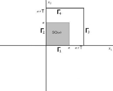
Figure 1: Geometry for the Inverse problem 2.

$$u=\frac{\partial u}{\partial\nu}=0\text{ on }\Gamma_{3T}\cup\Gamma_{4T}.$$ (1.7)

Hence, we focus our numerical study on

Inverse Problem 2. Let equation (1.1) be satisfied in $D_{T}^{3}$ with initial conditions (1.2) satisfying (1.4). In this case $\Omega:=SQ\left(a+T\right).$Suppose that one of these initial conditions is zero. Determine the second initial condition, assuming that functions $f$ and $g$ are known, where

$$u\mid_{\Gamma_{1T}\cup\Gamma_{2T}}=f\left(x,t\right),\text{ }\frac{\partial u}{\partial\nu}\mid_{\Gamma_{1T}\cup\Gamma_{2T}}=g\left(x,t\right).$$ (1.8)

Suppose for a moment that only the function $f\left(x,t\right)$ is given. Then one can solve the boundary value problem for equation (1.1) with $F\equiv 0$ outside of the square $SQ\left(a+T\right)$ with the following initial and boundary data

$$u\left(x,0\right)=u_{t}\left(x,0\right)=0,x\in R^{2}\diagdown SQ(a+T),$$

$$u\mid_{\Gamma_{1T}\cup\Gamma_{2T}}=f\left(x,t\right),u\mid_{\Gamma_{3T}\cup\Gamma_{4T}}=0\text{.}$$

This gives one in a stable way the normal derivative $g\left(x,t\right)$ on $\Gamma_{1T}\cup\Gamma_{2T}.$ Thus, we arrive at Inverse Problem 2. It was proven in [14] that if

$$T>\frac{a\sqrt{2}}{2-\sqrt{2}}$$ (1.9)

and one of functions $\varphi$ or $\psi$ equals zero, then the following Lipschitz stability estimate is valid

$$\left\|u\right\|_{H^{1}\left(G_{T}\right)}\leq C\left(\left\|f\right\|_{H^{1}\left(\Gamma_{T}\right)}+\left\|g\right\|_{L_{2}\left(\Gamma_{T}\right)}\right),$$ (1.10)

where $\Gamma_{T}=\Gamma_{1T}\cup\Gamma_{2T}$ and $\left\|f\right\|_{H^{1}\left(\Gamma_{T}\right)}=\left\|f\right\|_{H^{1}\left(\Gamma_{1T}\right)}+\left\|f\right\|_{H^{1}\left(\Gamma_{2T}\right)}.$ The estimate (1.10) implies a similar estimate for the unknown initial condition [14]. The knowledge of the fact that one of initial conditions was zero was used in [14] for either odd or even extension with respect to $t$ of the function $u(x,t)$ in $\left\{t<0\right\},$ depending on which of initial conditions was assumed to be unknown. The proof of [14] is based on the Carleman estimate. The method of Carleman estimates was first applied in [11] to obtain the Lipschitz stability for the hyperbolic problem with the lateral Cauchy data, also see [10] and Theorem 2.4.1 in [13]. Prior to [11] the Lipschitz stability for the hyperbolic problem with the lateral Cauchy data was obtained in [20] by the method of multipliers, but only for the case when lower order terms in (1.1) are absent. The use of the Carleman estimate enables one to incorporate lower order terms and also to extend to the case of hyperbolic inequalities. Recently the method of [10], [11], [13] was extended to hyperbolic equations with the non-constant principal part, see, e.g. [22]-[24]. The method of multipliers was recently extended to the case of non-zero lower order terms in Theorem 3.5 of the book [6].

The above problems were previously solved numerically in [4], [7], [12] and [15]. The work [7] was the first one, where the problem of thermoacoustic tomography was formulated and solved numerically as Inverse Problem 1, i.e., as the hyperbolic Cauchy problem with the lateral data. The QRM for the latter problem was used in [4]. The QRM was first proposed in the book [19] for a variety of ill-posed boundary value problems. Its convergence rates were established in [9] and [11] for the cases of Laplace and hyperbolic equations respectively and in section 2.5 of [13] for elliptic, parabolic and hyperbolic equations. In particular, it was shown in [13] that one can work with weak $H^{2}$ solutions of QRM instead of strong $H^{4}$ solutions of the original book [19]. Also, see [2] and [3] for the recent results for the QRM for the elliptic case and [8] for the application of the QRM to linearized coefficient inverse problems for parabolic equations. The main tool of works [4], [8], [9], [11] and [13] is the tool of Carleman estimates.

There are three main differences between the current paper and the previous works on the QRM for hyperbolic equations. First, we take into account boundary conditions via including them in the Tikhonov regularizing functional $J_{\varepsilon}$. Unlike this, boundary conditions were made zero in [4] via subtracting off a corresponding function, and they were treated via integration by parts in [12]. Second, we incorporate in $J_{\varepsilon}$ a penalizing term, which reflects our knowledge of one of initial conditions. We show numerically that without this term we cannot image well maximal values of the unknown initial condition inside of narrow peaks. On the other hand, since cancerous tumors can be modeled as narrow peaks, it is interesting to image those peaks in the application to thermoacoustic tomography considered below. These first two ideas for $J_{\varepsilon}$ are taken from [15]. Mainly because of the second difference we cannot apply previously derived convergence results and thus, need to prove convergence of our new version of the QRM. In particular, we need to prove a  new Lipschitz stability estimate (Theorem 4.1). Finally, the third difference is that while $H^{2}$ finite elements were used in [4] and [12], we use finite differences now. Note that while smooth slowly varying functions were reconstructed numerically in [4] and [12], our numerical experiments reconstruct both those functions and $\delta-$like functions. $\delta-$like functions were also reconstructed in [15] for the Inverse Problem 2. However, the numerical technique of [15] is different from one of the current paper. The method of [7] and [15] is based on the representation of the function $u(x,t)$ via truncated Fourier series and minimization of the resulting residual least squares functional.

In section 2 we describe applications of Inverse Problems 1 and 2. In section 3 we describe the version of the QRM we use here. In section 4 we prove a new Lipschitz stability estimate. In section 5 we prove convergence of our method, based on the result of section 4. In section 6 we describe our numerical implementation. In section 7 numerical results are presented. Conclusions are drawn in section 8.

2 Applications

In this section we discuss two applications of above inverse problems

2.1 Thermoacoustic tomography

Inverse Problems 1 and 2 arise in thermoacoustic tomography [4], [16], [25]. In  this case the target is subjected to a short electromagnetic impulse. The electromagnetic energy is absorbed. As a result, temperature is increased and the target is expanded. This causes a pressure wave, which is measured as a change in the acoustic field at the boundary of the sample. Assuming that the absorption of the electromagnetic energy is spatially varying inside the sample, the resulting wave field is carrying the signature of the inhomogeneity. On the other hand, cancerous regions absorb more than surroundings. This leads to applications in medical imaging. Hence, the problem is to calculate the absorption coefficient $\alpha(x)$ of the sample using time dependent measurements at its boundary. Let $\beta$ be the thermal expansion coefficient, $c_{p}$ be the specific capacity of the medium and $I_{0}$ be the power of the source. Usually $\beta,c_{p}$ and $I_{0}$ are known. Also, assume that the speed of sound in the medium is constant and equals 1. Let $u(x,t)$ be the pressure wave. It was shown in e.g., [4] that

$$u_{tt}=\Delta u,\left(x,t\right)\in\mathbb{R}^{3}\times\left(0,T\right),$$ (2.1)

$$u\left(x,0\right)=\alpha(x)I_{0}\frac{\beta}{c_{p}},\text{ \ }u_{t}\left(x,0\right)=0.$$ (2.2)

Suppose that we measure the function $u(x,t)$ at the boundary of the domain $\Omega$ and $\alpha(x)=0$ outside of $\Omega.$ Then those measurements give us the boundary value problem for equation (2.1) outside of $\Omega$ with zero initial conditions. Solving this problem, we uniquely determine the normal derivative of the function $u(x,t)$ at $\partial\Omega.$ Thus, we arrive at the $\varphi-$ problem.

A different approach to the problem of thermoacoustic tomography is currently actively developed in a number of publications. In this approach the solution of the problem (2.1), (2.2) is presented via the Poisson-Kirchhoff formula, which leads to the problem of integral geometry of recovering a function via its integrals over certain spheres, whose centers run over a surface and radii vary. Then uniqueness theorems are proven for this case and inversion formulas are derived, see, e,g., [1], [5], [16], and [17]. In particular, works [1] and [16] include the case of a variable speed and [16] and [17] include numerical examples. A survey of these developments can be found in [16]. Also, see §1 of Chapter 6 of the book [18] for an example of the ill-posedness of this integral geometry problem for the case when centers of spheres run over a plane in $\mathbb{R}^{3}$.

2.2 Linearized inverse acoustic and electromagnetic problems

There is also another application, in which Inverse Problems 1 and 2 can be considered as linearized inverse acoustic and inverse electromagnetic problems. The idea of this subsection is motivated by §1 of Chapter 7 of [18] and §3 of Chapter 2 of [21]. We present this application now without discussing delicate details about the validity of the linearization. In this setting the point source is running along a surface and time dependent measurements of back-reflected data are performed at the positions of the source. In [11] the Newton-Kantorovich method was presented for the case when the source position is fixed and the time dependent measurements are performed at a surface.

Let the function $\alpha\left(x\right)\in C\left(\mathbb{R}^{3}\right)$ be strictly positive, $\alpha\left(x\right)\geq const.>0.$ Consider the Cauchy problem for the hyperbolic equation

$$\alpha\left(x\right)w_{tt}=\Delta_{x}w+4\pi\delta\left(x-x_{0},t\right),\left(x,t\right)\in\mathbb{R}^{3}\times\left(0,T\right),$$ (2.3)

$$w\left(x,x_{0},0\right)=w_{t}\left(x,x_{0},0\right)=0,$$ (2.4)

where $x_{0}\in\mathbb{R}^{3}$ is the source position. It is well known that in acoustics $\alpha\left(x\right)=c^{-2}\left(x\right),$ where $c\left(x\right)$ is the speed of sound in the medium, and in some situations of the electromagnetics $\alpha\left(x\right)=\left(\mu\epsilon\right)\left(x\right),$ where $\mu$ and $\epsilon$ are respectively magnetic permeability and electric permittivity of the medium. We pose the following

Inverse Problem 3. Suppose that the function $\alpha\left(x\right)=1$ outside of the domain $\Omega$ and it is unknown inside of this domain. Determine this function for $x\in\Omega,$ assuming that the following function $p\left(x_{0},t\right)$ is known

$$w\left(x_{0},x_{0},t\right)\mid_{x_{0}\in\partial\Omega}=p\left(x_{0},t\right).$$ (2.4)

The full Inverse Problem 3 is difficult to address because of its nonlinearity. Hence, we consider now a linearized problem. Similarly with §3 of Chapter 2 of [21], suppose that the function $\alpha\left(x\right)$ can be represented in the form

$$\alpha\left(x\right)=1-\xi a\left(x\right),$$

where $\xi\in\left(0,1\right)$ is a small parameter. Hence, the term $\xi a\left(x\right)$ is a small perturbation of 1. We assume that this perturbation is unknown, i.e., the function $a\left(x\right)$ is unknown. Again, similarly with [21], we can formally set at $\xi\rightarrow 0$

$$w\left(x,x_{0},t\right)=w_{0}\left(x,x_{0},t\right)+\xi w_{1}\left(x,x_{0},t\right)+O\left(\xi^{2}\right),$$ (2.5)

where functions $w_{0}$ and $w_{1}$ are independent on $\xi.$ This setting was rigorously justified in §3 of Chapter 2 of [21] for the case of the telegraph equation

$$w_{tt}=\Delta w+\left(a_{0}\left(x\right)+\xi a_{1}\left(x\right)\right)w.$$ (2.6)

It was also justified in §1 of Chapter 7 of [18]for equation (2.6) without the introduction of the parameter $\xi,$ which is actually introduced here for convenience only. Indeed, instead, one can assume that $\alpha\left(x\right)=1-a\left(x\right),$ where $\left|a\left(x\right)\right|<<1.$

Substituting (2.6) in (2.3) and (2.4) and dropping the term with $O\left(\xi^{2}\right),$ we obtain that functions $w_{0}$ and $w_{1}$ are solutions of the following Cauchy problems

$$w_{0tt}=\Delta_{x}w_{0}+4\pi\delta\left(x-x_{0},t\right),\left(x,t\right)\in\mathbb{R}^{3}\times\left(0,T\right),$$ (2.7)

$$w_{0}\left(x,x_{0},0\right)=w_{0t}\left(x,x_{0},0\right)=0,$$ (2.8)

$$w_{1tt}=\Delta_{x}w_{1}+a\left(x\right)w_{0tt}\left(x,x_{0},t\right),\left(x,t\right)\in\mathbb{R}^{3}\times\left(0,T\right),$$ (2.9)

$$w_{0}\left(x,x_{0},0\right)=w_{t}\left(x,x_{0},0\right)=0.$$ (2.10)

Consider the function $h\left(x,x_{0},t\right),$

$$h\left(x,x_{0},t\right)=\int\limits_{0}^{t}d\tau\int\limits_{0}^{\tau}w_{1}\left(x,x_{0},s\right)ds.$$

Integrating (2.9) with respect to $t$ twice and using (2.8) and (2.10), we obtain

$$h_{tt}=\Delta_{x}h+a\left(x\right)w_{0}\left(x,x_{0},t\right),\left(x,t\right)\in\mathbb{R}^{3}\times\left(0,T\right),$$ (2.11)

$$h\left(x,x_{0},0\right)=h_{t}\left(x,x_{0},0\right)=0,$$ (2.12)

It follows from (2.7), (2.11), (2.12) and the formula (7.13) of §1 of Chapter 7 of [18] that the function $h\left(x,x_{0},t\right)$ is

$$h\left(x,x_{0},t\right)=\frac{1}{2\pi\left(t^{2}-\left|x-x_{0}\right|^{2}\right)}\int\limits_{S\left(x,x_{0},t\right)}\left|y-x_{0}\right|^{2}a\left(y\right)d\omega_{y},$$ (2.13)

where $d\omega_{y}=\sin\theta d\varphi d\theta,\left(\varphi,\theta\right)\in\left[0,2\pi\right]\times\left[0,\pi\right]$ are angles in the spherical coordinate system with the center at $\left\{x_{0}\right\}$ and $S\left(x,x_{0},t\right)$ is the following ellipsoid with foci at $\left\{x\right\}$ and $\left\{x_{0}\right\}$

$$S\left(x,x_{0},t\right)=\left\{y\in\mathbb{R}^{3}:\left|x-y\right|+\left|x_{0}-y\right|=t\right\}.$$

Setting in (2.13) $x_{0}:=x$ and denoting $v\left(x,t\right)=h\left(x,x,t\right),$ we obtain that the function $v$ is the spherical Radon transform of the function $a,$

$$v\left(x,t\right)=\frac{1}{4\pi}\int\limits_{\left|x-y\right|=t/2}a\left(y\right)d\omega_{y}.$$ (2.14)

On the other hand, (2.14) implies that the function $\widetilde{v}\left(x,t\right)=v\left(x,2t\right)\cdot t$ is the solution of the following Cauchy problem

$$\widetilde{v}_{tt}=\Delta\widetilde{v},\left(x,t\right)\in\mathbb{R}^{3}\times\left(0,2T\right).$$ (2.15)

$$\widetilde{v}\mid_{t=0}=0,\widetilde{v}_{t}\mid_{t=0}=a\left(x\right).$$ (2.16)

Also, using the above linearization one can “translate” the data $p\left(x_{0},t\right)$ in (2.4) for the Inverse Problem 3 in the following function $\widetilde{p}\left(x,t\right)$

$$\widetilde{v}\mid_{S_{T}}=\widetilde{p}\left(x,t\right),t\in\left(0,2T\right).$$ (2.17)

Since the function $a\left(x\right)=0$ outside of the domain $\Omega,$ then solving the initial boundary value problem (2.15)-(2.17) for $\left(x,t\right)\in\left(\mathbb{R}^{3}\diagdown\Omega\right)\times\left(0,T\right),$ we obtain the normal derivative $q\left(x,t\right),$

$$\frac{\partial\widetilde{v}}{\partial\nu}\mid_{S_{T}}=q\left(x,t\right),t\in\left(0,2T\right)$$ (2.18)

In conclusion, we have reduced the linearized Inverse Problem 3 to the $\psi-$problem, which consists in the recovery of the function $a\left(x\right)$ from conditions (2.15)-(2.18). A similar derivation is valid for a similar inverse problem for the telegraph equation (2.6) at $a_{0}\equiv 0,$ see [18] and [21].

3 The Method

We consider Inverse Problem 1, because it is more general than Inverse Problem 2. Denote $Mu=u_{tt}-Lu.$ To solve the Inverse Problem 1 numerically, consider the Tikhonov regularizing functional

$$J_{\varepsilon}\left(u\right)=\left\|Mu-F\right\|_{L_{2}\left(Q_{T}\right)}^{2}+\varepsilon\left\|u\right\|_{H^{2}\left(Q_{T}\right)}^{2}$$

$$+\left\|D^{\beta}u\mid_{S_{T}}-D^{\beta}f\right\|_{L_{2}\left(S_{T}\right)}^{2}+\left\|u_{\nu}\mid_{S_{T}}-g\right\|_{L_{2}\left(S_{T}\right)}^{2}$$ (3.1)

$$+\chi_{\varphi}\left\|u_{t}(x,0)-\psi\right\|_{L_{2}\left(\Omega\right)}^{2}+\chi_{\psi}\left\|u(x,0)-\varphi\right\|_{H^{1}\left(\Omega\right)}^{2},\forall u\in H^{2}\left(Q_{t}\right).$$

Here $\varepsilon>0$ is the regularization parameter,

$$u_{\nu}\mid_{S_{T}}:=\frac{\partial u}{\partial\nu}\mid_{S_{T}}$$

and $D^{\beta},\left|\beta\right|\leq 1$ is the operator of $\left(x,t\right)$ derivatives with, where $x$-derivatives are those, which are taken in directions orthogonal to the normal vector. Also,

$$\chi_{\psi}=\left\{\begin{array}[]{c}1\text{ for the }\psi-\text{problem}\\ 0\text{ for the }\varphi-\text{problem}\end{array}\right\},\chi_{\varphi}=\left\{\begin{array}[]{c}1\text{ for the }\varphi-\text{problem}\\ 0\text{ for the }\psi-\text{problem}\end{array}\right\}.$$

Hence, $\chi_{\varphi}\chi_{\psi}=0,\chi_{\varphi}+\chi_{\psi}=1.$ In previous works on the QRM terms in the second line of (3.1) were absent because of subtracting off boundary conditions from the original function $u$. Terms in the third line of (3.1) were absent also, and they are incorporated now to emphasize the knowledge of one of initial conditions.

To find the minimizer of $J_{\varepsilon}\left(u\right),$ we set the Fréchet derivative of this functional to zero and obtain for all $v\in H^{2}\left(Q_{T}\right)$

$$\int\limits_{Q_{T}}MuMvdxdt+\int\limits_{S_{T}}\left(D^{\beta}vD^{\beta}u+vu\right)\mid_{S_{T}}dS+\int\limits_{S_{T}}\left(v_{\nu}u_{\nu}\right)\mid_{S_{T}}dS$$

$$+\chi_{\psi}\int\limits_{\Omega}\left[\nabla u\nabla v+uv\right]\left(x,0\right)dx+\chi_{\varphi}\int\limits_{\Omega}u_{t}(x,0)v_{t}(x,0)dx+\varepsilon\left[u,v\right]$$ (3.2)

$$=\int\limits_{Q_{T}}FMvdxdt+\int\limits_{S_{T}}\sum\limits_{\left|\beta\right|\leq 1}\left(D^{\beta}v\mid_{S_{T}}\right)D^{\beta}fdS++\int\limits_{S_{T}}\left(v_{\nu}\mid_{S_{T}}\right)\cdot gdS$$

$$+\chi_{\psi}\int\limits_{\Omega}\left[\nabla\varphi\nabla v\left(x,0\right)+\varphi v\left(x,0\right)\right]dx+\chi_{\varphi}\int\limits_{\Omega}\psi v_{t}(x,0)dx.$$

Riesz theorem and (3.2) imply

Lemma 3.1. For any vector function $\left(F,f,g\right)\in L_{2}\left(Q_{T}\right)\times H^{1}\left(S_{T}\right)\times L_{2}\left(S_{T}\right)$ there exists unique solution $u_{\varepsilon}\in H^{2}\left(Q_{T}\right)$ of the problem (3.2) and

$$\left\|u_{\varepsilon}\right\|_{H^{2}\left(Q_{T}\right)}\leq\frac{C}{\sqrt{\varepsilon}}\left(\left\|F\right\|_{L_{2}\left(Q_{T}\right)}+\left\|f\right\|_{H^{1}\left(S_{T}\right)}+\left\|g\right\|_{L_{2}\left(S_{T}\right)}+\chi_{\psi}\left\|\varphi\right\|_{H^{1}\left(\Omega\right)}+\chi_{\varphi}\left\|\psi\right\|_{L_{2}\left(\Omega\right)}\right).$$

Setting in (3.2) $v:=u,$ we obtain that the unique minimizer of the functional $J_{\varepsilon}\left(u\right)$ satisfies the following estimate

$$\left\|Mu\right\|_{L_{2}\left(Q_{T}\right)}^{2}+\chi_{\psi}\left\|u(x,0)\right\|_{H^{1}\left(\Omega\right)}^{2}+\chi_{\varphi}\left\|u_{t}(x,0)\right\|_{L_{2}\left(\Omega\right)}^{2}$$

$$+\left\|u\mid_{S_{T}}\right\|_{H^{1}\left(S_{T}\right)}^{2}+\left\|u_{\nu}\mid_{S_{T}}\right\|_{L_{2}\left(S_{T}\right)}^{2}$$ (3.3)

$$\leq\left\|F\right\|_{L_{2}\left(Q_{T}\right)}^{2}+\left\|f\right\|_{H^{1}\left(S_{T}\right)}^{2}+\left\|g\right\|_{L_{2}\left(S_{T}\right)}^{2}+\chi_{\psi}\left\|\varphi\right\|_{H^{1}\left(\Omega\right)}^{2}+\chi_{\varphi}\left\|\psi\right\|_{H^{1}\left(\Omega\right)}^{2}.$$

To prove convergence of our method, we need to derive from (3.3) the Lipschitz stability estimate for the function $u$ in the $H^{1}\left(Q_{T}\right)$-norm. This in turn requires a modification of the proofs of [4], [10], [11] and [13]. We specifically refer to the proofs of Theorem 2.4.1 in [13] and Theorem 4.4 in [4]. The main difference with previous proofs is that now either $\left\|u(x,0)\right\|_{H^{1}\left(\Omega\right)}^{2}$ or $\left\|u_{t}(x,0)\right\|_{L_{2}\left(\Omega\right)}^{2}$ can be estimated via the right hand side of (3.3), which was not done before. This is because terms in the third line of (3.1) were not included in the Tikhonov functional for QRM. So, if $\chi_{\psi}=0,$ then $\chi_{\varphi}=1$ and we estimate $\left\|u(x,0)\right\|_{L_{2}\left(\Omega\right)}^{2}$ in the $\varphi-$problem. If, however, $\chi_{\psi}=1,$ then $\chi_{\varphi}=0$ and we estimate $\left\|u_{t}(x,0)\right\|_{L_{2}\left(\Omega\right)}^{2}$ in the $\psi$ problem. It is because of the incorporation of these terms that we can assume that $T>R$, as it is required in Inverse Problem 2 (see (1.9)), instead of $T>2R$ of previous works. The required modification is done in the next section.

4 Lipschitz Stability Estimate

Theorem 4.1. Let $\Omega\subset\mathbb{R}^{n}$ be a convex bounded domain with the piecewise smooth boundary and let $T>R$. Suppose that the function $u\in H^{2}\left(Q_{T}\right)$ satisfies the inequality

$$\left\|Mu\right\|_{L_{2}\left(Q_{T}\right)}+\chi_{\psi}\left\|u(x,0)\right\|_{H^{1}\left(\Omega\right)}+\chi_{\varphi}\left\|u_{t}(x,0)\right\|_{L_{2}\left(\Omega\right)}$$ (4.1)

$$+\left\|u\mid_{S_{T}}\right\|_{H^{1}\left(S_{T}\right)}+\left\|u_{\nu}\mid_{S_{T}}\right\|_{L_{2}\left(S_{T}\right)}\leq K,$$

where $K=const.>0$. Then

$$\left\|u\right\|_{H^{1}\left(Q_{T}\right)}+\chi_{\varphi}\left\|u\left(x,0\right)\right\|_{H^{1}\left(\Omega\right)}+\chi_{\psi}\left\|u_{t}\left(x,0\right)\right\|_{L_{2}\left(\Omega\right)}\leq CK.$$ (4.2)

Proof. Choose a pair of points $x^{\prime}$,$y^{\prime}\in\partial\Omega$ such that $\left|x^{\prime}-y^{\prime}\right|=2R.$ Put the origin at the point $\left(x+y\right)/2.$ Choose a constant $\eta\in\left(0,1\right)$. Consider the function $p\left(x,t\right),$

$$p\left(x,t\right)=\left|x\right|^{2}-\eta t^{2}.$$

Consider the Carleman Weight Function (CWF) $\mathcal{C}(x,t),$

$$\mathcal{C}(x,t)=\exp\left(2\lambda p\left(x,t\right)\right),$$

where $\lambda>1$ is a parameter. For any positive number $b$ denote

$G_{b}=\left\{\left(x,t\right)\mid p\left(x,t\right)>b,x\in\Omega,t>0\right\}.$ Choose a sufficiently small number $c\in\left(0,R^{2}\right).$ Since $T>R$, then in $G_{c}$

$$t^{2}<\frac{R^{2}-c}{\eta}<T^{2},\forall\eta\in\left(\eta_{0},1\right),$$

where $\eta_{0}=\eta_{0}\left(T,R\right)\in\left(0,1\right).$ Hence, $G_{c}\subset Q_{T}.$  Choose $\delta\in\left(0,c\right)$ so small that $G_{c+4\delta}\neq\varnothing.$ Note that

$$G_{c+4\delta}\subset G_{c+3\delta}\subset G_{c+2\delta}\subset G_{c+\delta}\subset G_{c}.$$ (4.3)

Denote $M_{0}u=u_{tt}-\Delta u.$ The following pointwise Carleman estimate takes place

$$\left(M_{0}u\right)^{2}\mathcal{C}^{2}\geq C\lambda\left(\left|\nabla_{x,t}u\right|^{2}+\lambda^{2}u^{2}\right)\mathcal{C}+\nabla\cdot U+V_{t}\text{ in }G_{c},\forall u\in C^{2}\left(\overline{G}_{c}\right),\forall\lambda>\lambda_{0},$$ (4.4)

where

$$\left|U\right|+\left|V\right|\leq C\lambda\left(\left|\nabla_{x,t}u\right|^{2}+\lambda^{2}u^{2}\right)\mathcal{C}\text{ in }G_{c}$$ (4.5)

and $\lambda_{0}\left(G_{c},\eta\right)>1$ is sufficiently large. In addition, the function $V$ is estimated as

$$\left|V\right|\leq C\lambda^{3}t\left(\left|\nabla_{x,t}u\right|^{2}+u^{2}\right)\mathcal{C}+C\lambda^{3}\left|u_{t}\right|\left(\left|\nabla u\right|+\left|u\right|\right)\mathcal{C}\text{ in }G_{c}.$$ (4.6)

This Carleman estimate was proven in Theorem 2.2.4 of [13]. It was derived earlier in §4 of Chapter 4 of [18].

Consider the cut-off function $\rho\left(x,t\right)\in C^{2}\left(\overline{G}_{c}\right)$ such that

$$\rho\left(x,t\right)=\left\{\begin{array}[]{c}1\text{ in }G_{c+2\delta}\\ 0\text{ in }G_{c}\diagdown G_{c+\delta}\\ \text{ between 0 and 1 otherwise}\end{array}\right\}.$$ (4.7)

The existence of such functions is well known. For an arbitrary function $u\in C^{2}\left(\overline{G}_{c}\right)$ denote $v=v(u):=\rho u.$ Using (4.4)-(4.6), we obtain

$$\int\limits_{G_{c}}\left(M_{0}v\right)^{2}\mathcal{C}dxdt\geq C\lambda\int\limits_{G_{c}}\left(\left|\nabla_{x,t}v\right|^{2}+\lambda^{2}v^{2}\right)\mathcal{C}dxdt$$

$$-C\lambda^{3}\int\limits_{\Omega}\left[\left|u_{t}\right|\left(\left|\nabla u\right|+\left|u\right|\right)\right]\left(x,0\right)\exp\left(2\lambda\left|x\right|^{2}\right)dx-C\lambda\int\limits_{S_{T}}\left[\left(D^{\beta}u\right)^{2}+\lambda^{2}u_{\nu}^{2}\right]\mathcal{C}dS.$$

Because by (4.3) $G_{c+2\delta}\subset G_{c},$ then (4.7) implies that the last inequality can be rewritten as

$$\int\limits_{G_{c}}\left(M_{0}v\right)^{2}\mathcal{C}dxdt\geq C\lambda\int\limits_{G_{c+2\delta}}\left(\left|\nabla_{x,t}u\right|^{2}+\lambda^{2}u^{2}\right)\mathcal{C}dxdt$$ (4.8)

$$-C\lambda^{3}\int\limits_{\Omega}\left[\left|u_{t}\right|\left(\left|\nabla u\right|+\left|u\right|\right)\right]\left(x,0\right)\exp\left(2\lambda\left|x\right|^{2}\right)dx-C\lambda\int\limits_{S_{T}}\left[\left(D^{\beta}u\right)^{2}+u_{\nu}^{2}\right]\mathcal{C}dS.$$

By (4.7) the left hand side of (4.8) can be estimated from the above as

$$\int\limits_{G_{c}}\left(M_{0}v\right)^{2}\mathcal{C}dxdt\leq\int\limits_{G_{c+2\delta}}\left(M_{0}u\right)^{2}\mathcal{C}dxdt+C\int\limits_{G_{c}\diagdown G_{c+2\delta}}\left(\left|\nabla_{x,t}u\right|^{2}+u^{2}\right)\mathcal{C}dxdt$$

$$\leq\int\limits_{G_{c+2\delta}}\left(M_{0}u\right)^{2}\mathcal{C}dxdt+C\lambda^{3}\left\|u\right\|_{H^{1}\left(Q_{T}\right)}^{2}\exp\left[2\lambda\left(c+2\delta\right)\right]$$

$$\leq\int\limits_{G_{c+2\delta}}\left(Mu\right)^{2}\mathcal{C}dxdt+C\int\limits_{G_{c+2\delta}}\left(\left|\nabla_{x,t}u\right|^{2}+u^{2}\right)\mathcal{C}dxdt+C\left\|u\right\|_{H^{1}\left(Q_{T}\right)}\exp\left[2\lambda\left(c+2\delta\right)\right].$$

Substituting this in (4.8), recalling that $\lambda$ is sufficiently large and using (4.3), we obtain

$$\int\limits_{G_{c+2\delta}}\left(Mu\right)^{2}\mathcal{C}dxdt+\lambda^{3}\left\|u\right\|_{H^{1}\left(Q_{T}\right)}^{2}\exp\left[2\lambda\left(c+2\delta\right)\right]$$

$$+\lambda\int\limits_{S_{T}}\left[\left(D^{\beta}u\right)^{2}+\lambda^{2}u_{\nu}^{2}\right]\mathcal{C}dS+\lambda^{3}\int\limits_{\Omega}\left[\left|u_{t}\right|\left(\left|\nabla u\right|+\left|u\right|\right)\right]\left(x,0\right)\exp\left(2\lambda\left|x\right|^{2}\right)dx$$

$$\geq C\lambda\int\limits_{G_{c+2\delta}}\left(\left|\nabla_{x,t}u\right|^{2}+\lambda^{2}u^{2}\right)\mathcal{C}dxdt\geq C\lambda^{3}\exp\left[2\lambda\left(c+3\delta\right)\right]\int\limits_{G_{c+3\delta}}\left(\left|\nabla_{x,t}u\right|^{2}+u^{2}\right)dxdt.$$

Let $m=\max_{\overline{G}_{c}}p(x,t).$ Dividing the last inequality by $C\lambda^{3}\exp\left[2\lambda\left(c+3\delta\right)\right],$ we obtain

$$\int\limits_{G_{c+3\delta}}\left(\left|\nabla_{x,t}u\right|^{2}+u^{2}\right)dxdt\leq$$

$$Ce^{2\lambda m}\left(\left\|Mu\right\|_{L_{2}\left(Q_{T}\right)}^{2}+\left\|u\mid_{S_{T}}\right\|_{H^{1}\left(S_{T}\right)}^{2}+\left\|u_{\nu}\mid_{S_{T}}\right\|_{L_{2}\left(S_{T}\right)}^{2}\right)+C\left\|u\right\|_{H^{1}\left(Q_{T}\right)}^{2}e^{-2\lambda\delta}$$ (4.9)

$$+Ce^{2\lambda m}\int\limits_{\Omega}\left[\left|u_{t}\right|\left(\left|\nabla u\right|+\left|u\right|\right)\right]\left(x,0\right)dx.$$

The last term of (4.9) was not present in previous publications, and we will analyze it now. Consider the $\varphi-$problem first. That is, consider the case $\chi_{\varphi}=1,\chi_{\psi}=0.$ Let $\gamma>0$ be a small number which we will choose later. We estimate the last term of (4.9) as

$$Ce^{2\lambda m}\int\limits_{\Omega}\left[\left|u_{t}\right|\left(\left|\nabla u\right|+\left|u\right|\right)\right]\left(x,0\right)dx$$

$$\leq C\gamma\int\limits_{\Omega}\left(\left|\nabla u\right|^{2}+u^{2}\right)\left(x,0\right)dx+\frac{Ce^{4\lambda m}}{\gamma}\int\limits_{\Omega}u_{t}^{2}\left(x,0\right)dx \varphi$$ (4.10)

$$\leq C\gamma\left\|u\left(x,0\right)\right\|_{H^{1}\left(\Omega\right)}^{2}+\frac{Ce^{4\lambda m}}{\gamma}K^{2}.$$

We have used (4.1) to estimate the last term in the second line of (4.10$\varphi$). Consider now the $\psi-$problem. Then similarly with (4.10$\varphi$)

$$Ce^{2\lambda m}\int\limits_{\Omega}\left[\left|u_{t}\right|\left(\left|\nabla u\right|+\left|u\right|\right)\right]\left(x,0\right)dx\leq C\gamma\left\|u_{t}\left(x,0\right)\right\|_{L_{2}\left(\Omega\right)}^{2}+\frac{Ce^{4\lambda m}}{\gamma}K^{2}. \psi$$ (4.10)

Consider now the set

$$F_{1}\left(c,\delta\right)=G_{c+3\delta}\cap\left\{t\in\left(0,\delta\right)\right\}.$$

Then

$$\left\{\left(x,t\right):\left|x\right|>\sqrt{c+3\delta+\eta\delta^{2}},x\in\Omega,t\in\left(0,\delta\right)\right\}\subset F_{1}\left(c,\delta\right).$$ (4.11)

Then (4.9), (4.10$\varphi)$ and (4.10$\psi)$ imply that

$$\int\limits_{F_{1}\left(c,\delta\right)}\left(\left|\nabla_{x,t}u\right|^{2}+u^{2}\right)dxdt\leq\frac{Ce^{4\lambda m}}{\gamma}K^{2}+C\left\|u\right\|_{H^{1}\left(Q_{T}\right)}^{2}e^{-2\lambda\delta}$$

$$+Ce^{2\lambda m}\left(\left\|u\mid_{S_{T}}\right\|_{H^{1}\left(S_{T}\right)}^{2}+\left\|u_{\nu}\mid_{S_{T}}\right\|_{L_{2}\left(S_{T}\right)}^{2}\right)$$

$$+\chi_{\varphi}C\gamma\left\|u\left(x,0\right)\right\|_{H^{1}\left(\Omega\right)}^{2}+\chi_{\psi}C\gamma\left\|u_{t}\left(x,0\right)\right\|_{L_{2}\left(\Omega\right)}^{2}.$$

Hence, by (4.1)

$$\int\limits_{F_{1}\left(c,\delta\right)}\left(\left|\nabla_{x,t}u\right|^{2}+u^{2}\right)dxdt\leq\frac{Ce^{4\lambda m}}{\gamma}K^{2}+C\left\|u\right\|_{H^{1}\left(Q_{T}\right)}^{2}e^{-2\lambda\delta}$$ (4.12)

$$+\chi_{\varphi}C\gamma\left\|u\left(x,0\right)\right\|_{H^{1}\left(\Omega\right)}^{2}+\chi_{\psi}C\gamma\left\|u_{t}\left(x,0\right)\right\|_{L_{2}\left(\Omega\right)}^{2}.$$

Choose numbers $c$ and $\delta$ so small that $3\sqrt{c+3\delta+\eta\delta^{2}}<R.$ Hence, we can choose $x_{0}\in\Omega$ such that $\left|x_{0}\right|=3\sqrt{c+3\delta+\eta\delta^{2}}.$ Next, we “shift” the function $p\left(x,t\right)$ to the point $x_{0},$ thus considering the function

$$p\left(x-x_{0},t\right)=\left|x-x_{0}\right|^{2}-\eta t^{2}.$$

For $b>0$ let $G_{b}\left(x_{0}\right)=\left\{\left(x,t\right)\mid p\left(x-x_{0},t\right)>b,x\in\Omega,t>0\right\}.$ Similarly with the above denote

$$F_{2}\left(c,\delta\right)=G_{c+3\delta}\left(x_{0}\right)\cap\left\{t\in\left(0,\delta\right)\right\}.$$

Then

$$\left\{\left(x,t\right):\left|x-x_{0}\right|>\sqrt{c+3\delta+\eta\delta^{2}},x\in\Omega,t\in\left(0,\delta\right)\right\}\subset F_{2}\left(c,\delta\right).$$ (4.13)

Consider an arbitrary point $x$ such that $x\in\left\{\left|x\right|<2\sqrt{c+3\delta+\eta\delta^{2}}\right\}.$ Then

$$\left|x_{0}-x\right|\geq\left|x_{0}\right|-\left|x\right|\geq 3\sqrt{c+3\delta+\eta\delta^{2}}-2\sqrt{c+3\delta+\eta\delta^{2}}=\sqrt{c+3\delta+\eta\delta^{2}}.$$

Hence, by (4.13)

$$\left\{\left(x,t\right):\left|x\right|<2\sqrt{c+3\delta+\eta\delta^{2}},t\in\left(0,\delta\right)\right\}\subset F_{2}\left(c,\delta\right).$$

Combining this with (4.11), we see that

$$\Omega\times\left(0,\delta\right)=Q_{\delta}\subset F_{1}\left(c,\delta\right)\cup F_{2}\left(c,\delta\right).$$ (4.14)

Using function $p\left(x-x_{0},t\right)$ instead of $p\left(x,t\right),$ we obtain similarly with (4.12)

$$\int\limits_{F_{2}\left(c,\delta\right)}\left(\left|\nabla_{x,t}u\right|^{2}+u^{2}\right)dxdt\leq\frac{Ce^{4\lambda m}}{\gamma}K^{2}+C\left\|u\right\|_{H^{1}\left(Q_{T}\right)}^{2}e^{-2\lambda\delta}$$

$$+\chi_{\varphi}C\gamma\left\|u\left(x,0\right)\right\|_{H^{1}\left(\Omega\right)}^{2}+\chi_{\psi}C\gamma\left\|u_{t}\left(x,0\right)\right\|_{L_{2}\left(\Omega\right)}^{2}.$$

Combining this with (4.12) and (4.14), we obtain

$$\left\|u\right\|_{H^{1}\left(Q_{\delta}\right)}\leq\frac{Ce^{4\lambda m}}{\gamma}K^{2}+C\left\|u\right\|_{H^{1}\left(Q_{T}\right)}^{2}e^{-2\lambda\delta}$$

$$+\chi_{\varphi}C\gamma\left\|u\left(x,0\right)\right\|_{H^{1}\left(\Omega\right)}^{2}+\chi_{\psi}C\gamma\left\|u_{t}\left(x,0\right)\right\|_{L_{2}\left(\Omega\right)}^{2}.$$

Hence, there exists a number $t^{\ast}\in\left(0,\delta\right)$ such that

$$\int\limits_{\Omega}\left(\left|\nabla_{x,t}u\right|^{2}+u^{2}\right)\left(x,t^{\ast}\right)dx\leq\frac{Ce^{4\lambda m}}{\delta\gamma}K^{2}+\frac{C}{\delta}\left\|u\right\|_{H^{1}\left(Q_{T}\right)}^{2}e^{-2\lambda\delta}$$

$$+\frac{1}{\delta}\left[\chi_{\varphi}C\gamma\left\|u\left(x,0\right)\right\|_{H^{1}\left(\Omega\right)}^{2}+\chi_{\psi}C\gamma\left\|u_{t}\left(x,0\right)\right\|_{L_{2}\left(\Omega\right)}^{2}\right].$$

This inequality combined with (4.1) and the standard energy estimates implies that

$$\left\|u\right\|_{H^{1}\left(Q_{T}\right)}^{2}+\chi_{\varphi}\left\|u\left(x,0\right)\right\|_{H^{1}\left(\Omega\right)}^{2}+\chi_{\psi}\left\|u_{t}\left(x,0\right)\right\|_{L_{2}\left(\Omega\right)}^{2}\leq C\left\|u\right\|_{H^{1}\left(Q_{T}\right)}^{2}e^{-2\lambda\delta}$$

$$+\frac{Ce^{4\lambda m}}{\gamma}K^{2}+\chi_{\varphi}C\gamma\left\|u\left(x,0\right)\right\|_{H^{1}\left(\Omega\right)}^{2}+\chi_{\psi}C\gamma\left\|u_{t}\left(x,0\right)\right\|_{L_{2}\left(\Omega\right)}^{2}.$$ (4.15)

Note that $\delta$ is independent on $\lambda.$ Choose sufficiently large $\lambda_{0}$ such that

$$1-Ce^{-2\lambda_{0}\delta}>\frac{1}{2}$$

and set $\lambda:=\lambda_{0}.$ Choose $\gamma$ so small that $C\gamma<1/2.$ Then we obtain (4.2) from (4.15). $\square$

5 Convergence

Theorem 4.1 enables us to prove convergence of our method. Following the Tikhonov concept for ill-posed problems [18], we first introduce an “ideal” exact solution of either $\varphi$ or $\psi$ problem without an error in the data. Next, we assume the existence of the error in  the boundary data $f$ and $g$ and prove that our solution tends to the exact one as the level of error in the data tends to zero. We consider the more general Inverse Problem 1. Let $f^{\ast}\in H^{1}\left(S_{T}\right)$ and $g^{\ast}\in L_{2}\left(S_{T}\right)$ be the exact boundary data (1.3), $F^{\ast}\in L_{2}\left(Q_{T}\right)$ be the exact right hand side of equation (1.1) and $\varphi^{\ast}$ and $\psi^{\ast}$ be exact initial conditions. We assume that there exists an exact function $u^{\ast}\in H^{2}\left(Q_{T}\right)$ satisfying

$$u_{tt}^{\ast}=L(x,t)u^{\ast}+F^{\ast}\left(x,t\right)\text{ in }Q_{T},$$ (5.1)

with initial conditions

$$u^{\ast}\left(x,0\right)=\varphi^{\ast}\left(x\right),u_{t}^{\ast}\left(x,0\right)=\psi^{\ast}\left(x\right),\varphi^{\ast}\in H^{1}\left(\Omega\right),\psi^{\ast}\in L_{2}\left(\Omega\right),$$ (5.2)

$$u^{\ast}\mid_{S_{T}}=f^{\ast}\left(x,t\right),\frac{\partial u^{\ast}}{\partial\nu}\mid_{S_{T}}=g^{\ast}\left(x,t\right),$$ (5.3)

where $\varphi^{\ast}$ and $\psi^{\ast}$ are exact initial conditions. We assume that the real boundary data in (1.3) have an error, so as the given initial condition. In other words, we assume that

$$\left\|f-f^{\ast}\right\|_{H^{1}\left(S_{T}\right)}+\left\|g-g^{\ast}\right\|_{L_{2}\left(S_{T}\right)}+\left\|F-F^{\ast}\right\|_{L_{2}\left(Q_{T}\right)}$$ (5.4)

$$+\chi_{\psi}\left\|\varphi-\varphi^{\ast}\right\|_{H^{1}\left(\Omega\right)}+\chi_{\varphi}\left\|\psi-\psi^{\ast}\right\|_{L_{2}\left(\Omega\right)}\leq\delta,$$

where $\delta>0$ is a small number. The following convergence theorem holds

Theorem 5.1. Suppose that $T>R.$ Let $u_{\varepsilon\delta}\in H^{2}\left(Q_{T}\right)$ be the solution of the QRM problem (3.2), which is guaranteed by Lemma 2.1. Let conditions (5.1)-(5.4) be satisfied. Then the following estimate is valid

$$\left\|u-u^{\ast}\right\|_{H^{1}\left(Q_{T}\right)}+\chi_{\varphi}\left\|\varphi-\varphi^{\ast}\right\|_{H^{1}\left(\Omega\right)}+\chi_{\psi}\left\|\psi-\psi^{\ast}\right\|_{L_{2}\left(\Omega\right)}\leq C\left(\delta+\sqrt{\varepsilon}\right).$$

Proof. Since the functional $J_{0}\left(u\right)$ with the exact data (5.2), (5.3) achieves its minimal zero value at $u:=u^{\ast},$ then the function $u^{\ast}$ satisfies equation (3.2) with $\varepsilon=0$ and with the exact data (5.2), (5.3). Subtracting that equation for $u^{\ast}$ from equation  (3.2) for $u:=u_{\varepsilon\delta},$ denoting $w=u_{\varepsilon\delta}-u^{\ast}$, setting in resulting equation $v:=w$ and using (5.4), we obtain similarly with (3.3)

$$\int\limits_{Q_{T}}\left(Mw\right)^{2}dxdt+\chi_{\psi}\left\|w(x,0)\right\|_{H^{1}\left(\Omega\right)}^{2}+\chi_{\varphi}\left\|w_{t}(x,0)\right\|_{L_{2}\left(\Omega\right)}^{2}$$

$$+\left\|w\mid_{S_{T}}\right\|_{H^{1}\left(S_{T}\right)}^{2}+\left\|w_{\nu}\mid_{S_{T}}\right\|_{L_{2}\left(S_{T}\right)}^{2}\leq 4\delta^{2}+\varepsilon.$$

The  rest of the proof follows immediately from Theorem 4.1. $\square$

6 Numerical Implementation

In our numerical study we have considered the Inverse Problem 2. To generate the data for the inverse problem, we have solved the Cauchy problem

$$u_{tt}=\Delta u,\left(x,t\right)\in\mathbb{R}^{2}\times\left(0,T\right),$$ (6.1)

$$u(x,0)=\varphi\left(x\right),u_{t}(x,0)=\psi\left(x\right).$$ (6.2)

In our numerical experiments $\psi\left(x\right)\equiv 0$ for the $\varphi-$problem, and $\varphi\left(x\right)\equiv 0$ for the $\psi-$problem. Because of (1.5) and the finite speed of propagation, we use in our solution of the forward problem zero Dirichlet boundary condition at the boundary of the rectangle $\left(-T,a+T\right)\times\left(-T,a+T\right)$ (Figure 1). Hence, we solve initial boundary value problem inside of this rectangle for equation (6.1) with initial conditions (6.2) at zero Dirichlet boundary condition. In all our calculations we took $a=1.$ In tests 1, 2 and 5, which are concerned with the Inverse Problem 2, we took $T=3.$ Hence, condition (1.9) is satisfied. Tests 3 and 4 are concerned with the Inverse Problem 1 and we have taken different values of $T$ in these tests. The square $SQ(a)$ is $SQ(a)=SQ(1)=\left(0,1\right)\times\left(0,1\right),$ the domain $\Omega$ in tests 1,2 and 5 is

$$\Omega:=\left(0,4\right)\times\left(0,4\right)$$ (6.3)

and in all tests

$$\varphi\left(x\right)=\psi\left(x\right)=0\text{ for }x\notin SQ(1).$$ (6.4)

We have solved the Cauchy problem (6.1), (6.2) via finite differences using the uniform grid. We set

$$u(t_{k},x_{1n},x_{2m})\approx u_{kmn},\,k=0,...,N_{t},\,\,n=0,...,N_{x},m=0,...,N_{y},$$

$$t_{k}=kh_{t},\,x_{1n}=nh_{x_{1}},\,x_{2m}=mh_{x_{2}},$$

step sizes $h_{x_{1}}=h_{x_{2}}=0.1,h_{t}=1/15$ and $N_{x}=N_{y}=10,N_{t}=45$. This solution has generated the boundary data (1.8). Next, we have introduced noise in these data as

$$f_{n}\left(x^{i},t_{j}\right)=f\left(x^{i},t_{j}\right)\left(1+\gamma N\left(t_{j}\right)\right),g_{n}\left(x^{i},t_{j}\right)=g\left(x^{i},t_{j}\right)\left(1+\gamma N\left(t_{j}\right)\right),$$ (6.5)

where $\left(x^{i},t_{j}\right)$ is the grid point at the boundary. Here $N\in\left(-1,1\right)$ is a pseudo random variable, which is given by function $Math.random()$ in Java and $\gamma\in\left[0.05,0.5\right]$ is the noise level. We have chosen the grid points the same as ones in the finite difference scheme we have solved the problem (6.1), (6.2). The presence of the random noise in the date prevents us from committing “inverse crime”. In (6.5) points $x^{i}\in\Gamma_{1T}\cup\Gamma_{2T}.$ As to $\Gamma_{3T}\cup\Gamma_{4T},$ we simply set $f=g=0$ on this part of the boundary, because of (1.7).

To find the minimizer of the functional $J_{\varepsilon},$ we have also used finite differences. We have used in (3.1) the finite difference approximations for $Mu=u_{tt}-\Delta u$ and $u_{\nu}\mid_{S_{T}}$ and have minimized the resulting functional $\widetilde{J}_{\varepsilon}$ with respect to the vector $\left\{u_{kmn}\right\},$ which approximates values of the function $u$ at grid points. Here $\widetilde{J}_{\varepsilon}$ means the functional $J_{\varepsilon},$ which is expressed via the finite differences. The norms $\left\|u_{x_{1}}(x,0)\right\|_{L_{2}\left(\Omega\right)},$ $\left\|u_{x_{2}}(x,0)\right\|_{L_{2}\left(\Omega\right)}$ in $\left\|u(x,0)\right\|_{H^{1}\left(\Omega\right)}$ in the $\psi-$problem were calculated via finite differences. As to the term $\left\|D^{\beta}u\mid_{S_{T}}-D^{\beta}f\right\|_{L_{2}\left(S_{T}\right)}^{2}$ in (3.1), we have used only $\beta=0,$ thus ending up with $\left\|u\mid_{S_{T}}-f\right\|_{L_{2}\left(S_{T}\right)}^{2}$ (in the discrete sense). Note that since $\beta=0,$ our numerical results seem to be stronger than Theorem 4.1 predicts. The integrals were calculated as

$$\int\limits_{\Omega_{T}}(u_{tt}-\Delta u)^{2}dv\approx\frac{h_{t}h_{x_{2}}h_{x_{1}}}{h_{t}^{4}}\sum_{k=1}^{N_{t}-1}\sum_{m=1}^{N_{y}-1}\sum_{n=1}^{N_{x}-1}M_{kmn}^{2},$$

where

$$M_{kmn}=(u_{k+1,mn}-2u_{kmn}+u_{k-1,mn})-\lambda_{y}(u_{k,m+1,n}-2u_{kmn}+u_{k,m-1,n})\\ -\lambda_{x}\left(u_{km,n+1}-2u_{kmn}+u_{km,n-1}\right)\\ =(u_{k+1,mn}+u_{k-1,mn})-\lambda_{y}(u_{k,m+1,n}+u_{k,m-1,n})-\lambda_{x}(u_{km,n+1}+u_{km,n-1})-\lambda_{t}u_{kmn},$$

where

$$\lambda_{x}=\frac{h_{t}^{2}}{h_{x_{1}}^{2}},\quad\lambda_{y}=\frac{h_{t}^{2}}{h_{x_{2}}^{2}},\quad\lambda_{t}=2(1-\lambda_{x}-\lambda_{y}).$$

Also,

$$\int\limits_{0}^{T}\int\limits_{0}^{a+T}(u(t,x_{2},x_{1}^{\ast})-f(t,x_{2}))^{2}dx_{2}dt\approx h_{t}h_{x_{2}}\sum_{k=0}^{N_{t}}\sum_{m=0}^{N_{x_{2}}}H_{km}^{2},$$

where

$$H_{km}=u_{kmn_{\ast}}-h_{km},$$

where $n_{\ast}$ in the layer number (value of $x_{1}^{\ast}$) at which the grid function $f_{km}$ is given.

To minimize the functional $\widetilde{J}_{\varepsilon},$ we have used the conjugate gradient method. Derivatives with respect to variables $u_{kmn}$ where calculated in closed forms, using the following formula

$$\frac{\partial u_{kmn}}{\partial u_{\overline{k}\overline{m}\overline{n}}}=\delta_{k\overline{k}}\delta_{m\overline{m}}\delta_{n\overline{n}},$$

where $\delta_{k\overline{k}}$ is the Kronecker symbol. This formula can be conveniently used to obtain closed form expressions for derivatives

$$\frac{\partial\widetilde{J}_{\varepsilon}\left(u\right)}{\partial u_{kmn}}.$$

Let $a$ be the vector of unknowns of the functional $\widetilde{J}_{\varepsilon}$. We start our iterative process from $a:=a_{0}=0$. It is well known in the field of ill-posed problems that the number of iterations can often be taken as a regularization parameter, and it depends, of course on the range of parameters of a problem one considers. We have found that the optimal number of iterations for our range of parameters is $300$. Thus, in all numerical examples below 300 iterations of the conjugate gradient method were used, thus ending up with $a_{300}$. Figure 2 displays typical dependencies of the functional $\widetilde{J}_{\varepsilon}\left(a_{k}\right)$ and the norm of its gradient on the iteration number $k$.

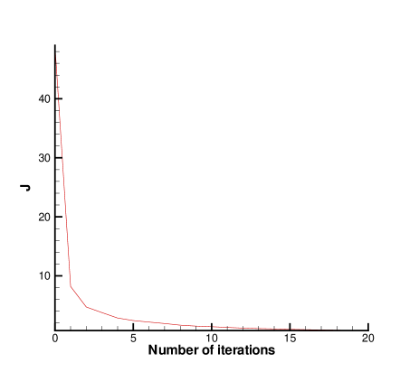
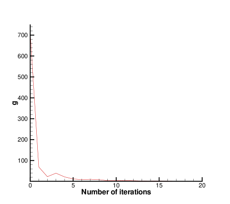
Figure 2: Typical dependence of the functional $J=J_{\varepsilon}$ (left) and $g=\|\nabla J_{\varepsilon}\|^{2}$ (right) on number of iterations.

7 Numerical Results

In this section we present results of some numerical experiments. We have always used $\varepsilon=10^{-6}.$ Larger values of $\varepsilon$ such as $10^{-5}$ brought lower quality results. In our numerical experiments we have imaged both smooth slowly varying functions and the finite difference analogue of the $\delta-$ function. Let $\left(x_{1k},x_{2r}\right)\in\Omega$ be a fixed grid point. To obtain the finite difference analogue of $\delta\left(x_{1}-x_{1k},x_{2}-x_{2r}\right)$, we consider the following grid points $\left(x_{1n},x_{2m}\right)$ and we model the function $\delta\left(x_{1n}-x_{1k},x_{2m}-x_{2r}\right)$ as

$$\delta\left(x_{1n}-x_{1k},x_{2m}-x_{2r}\right)=\frac{3}{4h_{x_{2}}h_{x_{1}}}\delta_{nk}\delta_{mr},$$

where the multiplier at $\delta_{nk}\delta_{mr}$ is chosen such that the volume of the pyramid based on $\left(x_{1k-1},x_{2r-1}\right),\,\left(x_{1k-1},x_{2r+1}\right),\,\left(x_{1k+1},x_{2r+1}\right),\,\left(x_{1k+1},x_{2r-1}\right)$ equals to $1$. Hence, the support of the function $\delta\left(x_{1n}-x_{1k},x_{2m}-x_{2r}\right)$ is limited only to the point $\left(x_{1n},x_{2m}\right)$.

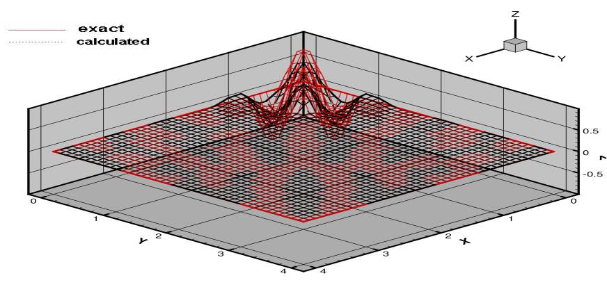
Figure 3: Exact (red) and calculated (black) functions $\varphi$ in (7.1) without balancing coefficients with 5% noise in boundary data.

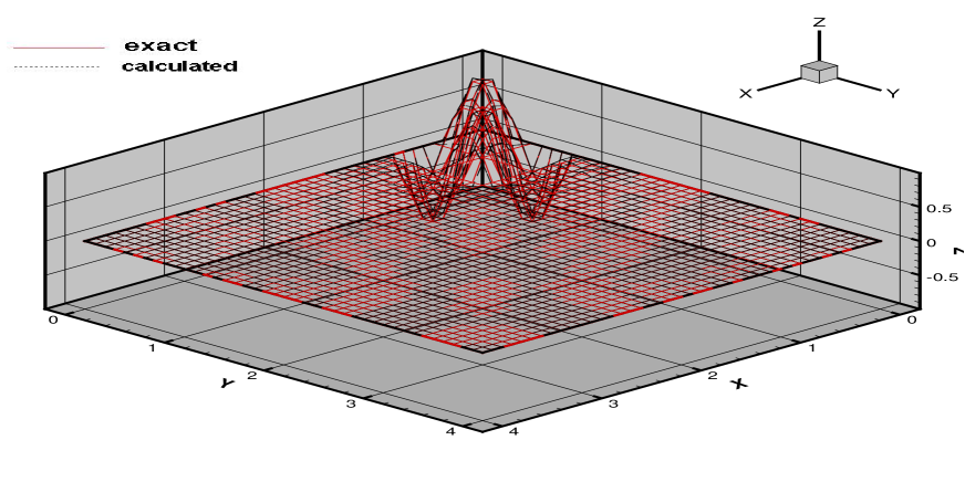
Figure 4: Exact (red) and calculated (black) functions $\varphi$ in (7.1) with balancing coefficients with 5% noise in boundary data.

We have observed that having equal coefficient at all terms of the functional $\widetilde{J}_{\varepsilon}$ in (3.1) does not lead to good reconstruction results. This is because not all the terms of (3.1) provide an equal impact in this functional. For example, for the $\varphi-$problem with no noise in the data for the function

$$\varphi\left(x\right)=\left\{\begin{array}[]{c}\sin(2\pi x_{1})\sin(2\pi x_{2}),x\in SQ\left(1\right)\\ 0\text{ otherwise}\end{array}\right\}$$ (7.1)

we first got the result displayed in Figure 3. One can observe that the error at the boundary is significant. And indeed, the values of two terms in (3.1) after 300 iterations were for this case

$$\int\limits_{\Omega_{T}}(u_{tt}-\Delta u)^{2}dxdt\approx 10^{-3},\quad\|u-f\|_{L_{2}(S_{T})}\approx 10^{-2}.$$

Hence, the impact of the boundary term in (3.1) is 10 greater than the impact of the $\left\|Mu\right\|_{L_{2}\left(Q_{T}\right)}^{2}.$ To minimize the error at the boundary, we took the balancing coefficient $1000$ at $1000\cdot\|u-f\|_{L_{2}(S_{T})}$ instead of $1\cdot\|u-f\|_{L_{2}(S_{T})}$. The other balancing coefficients equal to $1$. The quality of the resulting image was improved, see Figure 4. Thus, in all our tests with the $\varphi-$problem we have taken the same balancing coefficients. In the case of the $\psi-$problem we have taken $100\cdot\chi_{\psi}\left\|u(x,0)-\varphi\right\|_{H^{1}\left(\Omega\right)}^{2}$ and the other balancing coefficients equal to $1$.

Note that Theorems 4.1 and 5.1 remain the same, including their proofs, if balancing coefficients are introduced.

Test 1. The $\varphi-$problem. Here $\psi\left(x\right)\equiv 0$ and the function $\varphi\left(x\right)$ to be reconstructed is one in (7.1). In Figures 5 and 6 represent resulting images with 25% and 50% noise respectively. Next, we test our method for the case when the term with $\chi_{\varphi}$ is absent in the functional $J_{\varepsilon}\left(u\right)$ in (3.1). Regardless on the small amount of noise in the data, both maximal ($1$) and minimal ($-1$) values of the imaged function were missed by about 22% in this case, whereas they were not missed in the previous cases with 25% and 50% noise when the term with $\chi_{\varphi}$ was not absent in (3.1). To see this, we display on Figure 7 the 1-dimensional cross-sections by the straight line $\left\{x_{1}=0.5\right\}$ of the correct function (7.1), the imaged function with 50% noise of Figure 6 and the imaged function with the absent term with $\chi_{\varphi}$ and 5% noise. One can observe that the maximal value of the calculated function is $0.7$, while the maximal absolute value of the correct function is $0.9$, so as the one of Figure 6. Here we have $0.9$ instead of $1$ only because the points with the absolute value of $1$ are not the grid points.  This emphasizes the importance of the incorporation of the term with $\chi_{\varphi}.$ We have observed the same for the $\psi-$ problem (images not shown).

Figure 5: Test 1. Exact (red) and calculated (black) functions $\varphi$ in (7.1) with 25% noise in the boundary data.

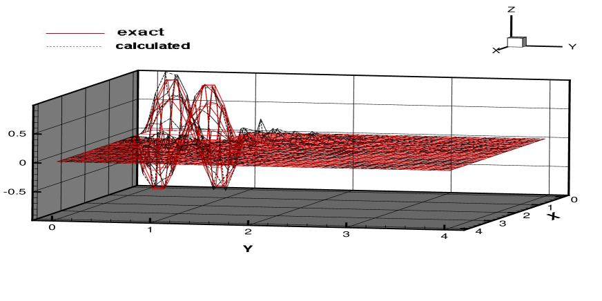
Figure 6: Test 1. Exact (red) and calculated (black) functions $\varphi$ in (7.1) with 50% noise in the boundary data.

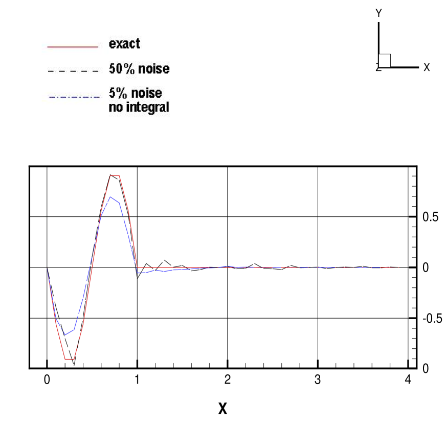
Figure 7: Test 1. Cross sections of exact (red) and calculated (black, blue) functions $\varphi$ with 5%, 50% noise, ”no integral” means $\chi_{\varphi=0}$. One can see that the maximal value of the case $\chi_{\varphi=0}$ is $0.7/(-0.7)$. The maximal value of the exact function is $0.9<1$ only because of the grid step size.

Test 2. The $\psi-$problem. In this case $\varphi\left(x\right)\equiv 0$ and the function $\psi\left(x\right)$ to be reconstructed is

$$\psi\left(x\right)=\left\{\begin{array}[]{c}\sin(\frac{\pi}{2}\left(x_{1}-0.5\right)\sin(\frac{\pi}{2}\left(x_{2}-0.5\right)),x\in SQ\left(1\right)\\ 0\text{ otherwise.}\end{array}\right\}.$$ (7.2)

Figures 8, 9 and 10display resulting images of the function (7.2) with 5%, 25% and 50% of the noise level in the data respectively.

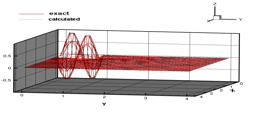
Figure 8: Test 2. Exact (red) and calculated (black) functions $\psi$ in (7.2) with 5% noise in the boundary data.

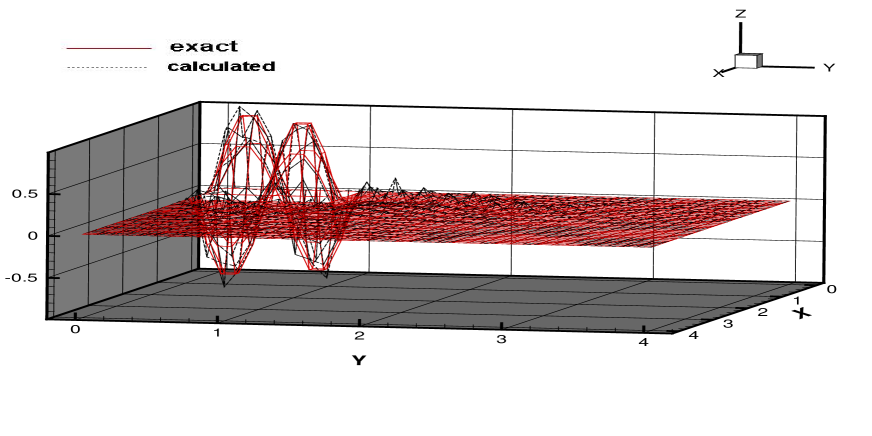
Figure 9: Test 2. Exact (red) and calculated (black) functions $\psi$ in (7.2) with 25% noise in the boundary data.

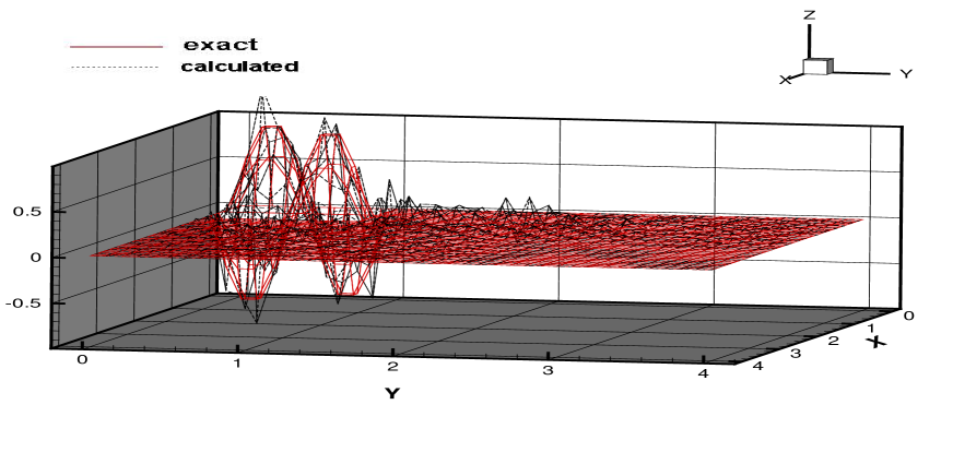
Figure 10: Test 2. Exact (red) and calculated (black) functions $\psi$ with 50% noise in the boundary data.

Test 3. The $\varphi-$problem in $SQ(1)$ for $T\in\left(0.5diam\,SQ\left(1\right),diam\,SQ\left(1\right)\right),$ where $diam\,SQ\left(1\right)=\sqrt{2}$ is the diameter of the square $SQ\left(1\right)$. We have decided to see what kind of results can be obtained if the boundary Cauchy data are given on the entire boundary of the square $SQ\left(1\right)$ in the case when $\,T\in\left(0.5diam\,SQ\left(1\right),diam\,SQ\left(1\right)\right).$ We are especially interested in the question about the influence of terms with $\chi_{\varphi}$ and $\chi_{\psi}.$ We have used

$$\,T=0.75<diam\,SQ\left(1\right)=\sqrt{2},N_{x}=N_{y}=20,\,N_{t}=3.$$

and have reconstructed the function (7.1). Figure 11 displays the resulting image with $25\%$ noise in the case when the term $\chi_{\varphi}$ is present in (3.1). This quality of the reconstruction is good for such a high noise level. Figure 12 displays the 1-dimensional cross-section of the image by the straight line $\left\{x_{1}=0.5\right\}$, as well as the 1-dimensional cross-section of the image for the case when the term with $\chi_{\varphi}$ is not present in (3.1) and 25% noise in the data is in. One can observe that the minimal value of $(-0.9)$ is not achieved in the case when the term with $\chi_{\varphi}$ is not present. The calculated minimal value is $(-0.7)$ in this case.

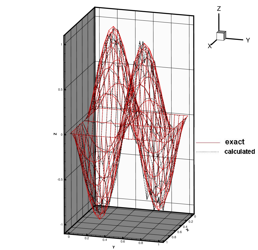
Figure 11: Test 3. Exact (red) and calculated (black) solutions of the problem $\varphi-$ in SQ(1) with 25% noise in the boundary data for $T=0.75$.

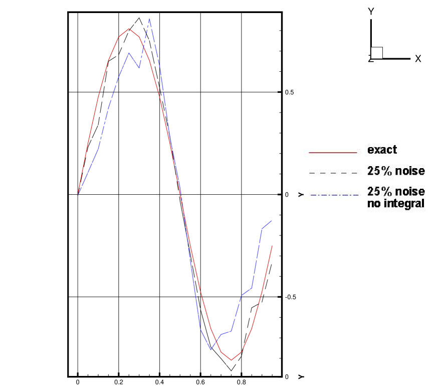
Figure 12: Test 3. Cross sections of exact (red) and calculated (black, blue) functions $\varphi$ with 25% noise in the boundary data for $T=0.75$, ”no integral” means $\chi_{\varphi}=0$. The maximal value of the exact function is $0.9<1$ only because of the grid step size.

Test 4. The $\varphi-$problem in $SQ(1)$ for $T>diam\,SQ\left(1\right)$. We now test our method for the case when the boundary Cauchy data are given at the entire boundary of the rectangle $SQ\left(1\right)$ and $T>diam\,SQ\left(1\right)$. We take

$$T=2,\,N_{x}=N_{y}=20,\,N_{t}=60.$$

The function (7.1) was reconstructed. Figure 13 displays the resulting image with $25\%$ noise and Figure 14 displays the 1-dimensional cross-section of the image by the straight line $\left\{x_{1}=0.5\right\}$, as well as the 1-dimensional cross-section of the image for the case when the term with $\chi_{\varphi}$ is not present in (3.1) (with 25% noise). One can observe that both images are very close to the correct one. This points towards the fact, which follows from the theory of above cited publications and also from Theorem 4.1: the presence of terms with $\chi_{\varphi}$ and $\chi_{\psi}$ is important only when $T\in\left(R,2R\right)$ and it is unimportant for $T>2R.$

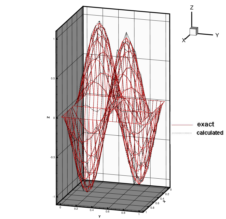
Figure 13: Test 4. Exact (red) and calculated (black) solutions of the $\varphi-$ problem in SQ(1) with 25% noise in the boundary data for $T=2$.

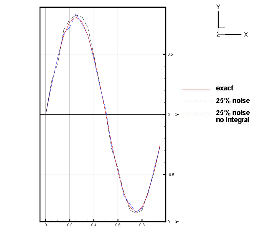
Figure 14: Test 4. Cross sections of exact (red) and calculated (black, blue) functions $\varphi$ with 25% noise in the boundary data for $T=0.75$, ”no integral” means $\chi_{\varphi}=0$. The maximal value of the exact function is $0.9<1$ only because of the grid step size.

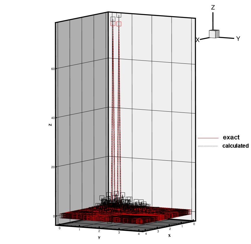
Figure 15: Test 5. Exact (red) and calculated (black) function $\varphi$ with 50% noise in the boundary data. The function $\chi_{\varphi}$ in (3.1) is present. Scatter plot mode. Squares show heights. Correct heights are achieved.

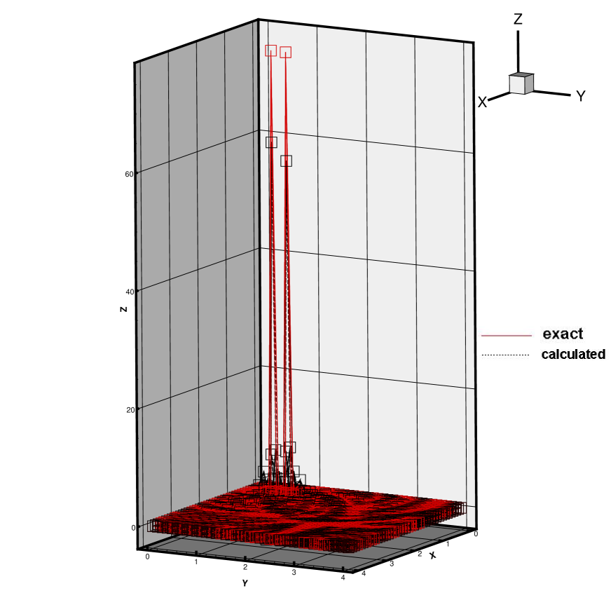
Figure 16: Test 5. Exact (red) and calculated (black) function $\varphi$ with 5% noise in the boundary data and $\chi_{\varphi}=0$. Scatter plot mode. Squares show heights. Correct heights are not achieved.

Test 5. The $\varphi-$problem with two $\delta-$functions. We now again consider the Inverse Problem 2 with the domain $\Omega$ as in (6.3) and with $\psi(x)\equiv 0.$ The data for the forward problem were simulated for the case

$$\varphi\left(x_{1},x_{2}\right)=\delta\left(x_{1}-0.4,x_{2}-0.4\right)+\delta\left(x_{1}-0.7,x_{2}-0.7\right)$$ (7.3)

with the above described finite difference analogue of the $\delta-$ function. Figure 15 displays the resulting image of the function (7.3) for the case of 50% of the noise in the boundary data, scatter plot mode was used, squares show exact height. Figure 16, on the other hand, shows the image when the term with $\chi_{\varphi}$ is absent in (3.1) and only 5% noise in the data is present. One can see that the correct height is not reached on Figure 16, unlike Figure 15. This again shows the importance of the introduction of terms in the third line of (3.1).

Very similar results (not shown) were obtained for the $\psi-$problem with exactly the same $\delta-$ functions as ones in (7.3).

8 Conclusions

We have considered the inverse problems of the determination of one of initial condition in a hyperbolic equation using the lateral Cauchy data. We have presented applications of these problems to the thermoacoustic tomography, as well as to linearized inverse acoustic and inverse electromagnetic problems. The problems we consider are very close ones with the Cauchy problems for hyperbolic equations with the lateral data, and we have actually solved the latter numerically in Tests 3 and 4. We have focused on the inverse problem in an infinite domain (octant), whereas only finite domains were considered in previous numerical studies. Nevertheless, we are able to reduce our inverse problem to one in a finite domain due to the finite speed of propagation of waves. Since one initial condition is known, we were able to decrease the observation time $T$ by twofold. We have shown numerically that it is important to know one of initial conditions if $T<diameter\left(\Omega\right),$ as it is required by stability and uniqueness results. However, if $T>diameter\left(\Omega\right),$ then both the theory and our numerical result of Test 4 show that one does not need to know the initial condition.

We have proposed a new version of the Quasi-Reversibility method. The main new element of this version is the inclusion of the terms characterizing a priori knowledge of one of initial conditions. Two other new elements are incorporation of boundary terms in the Tikhonov functional instead of subtracting off boundary conditions and the use of finite differences instead of finite elements in the inverse solver. To prove convergence of this new version, we have modified the technique of previous works, which is based on Carleman estimates. A comprehensive numerical study of the proposed numerical method was conducted. This study has demonstrated robustness of our technique with respect up to 50% random noise in the data, similarly with previous publications [4], [12], [15]. This study has also demonstrated that this method is capable to image sharp peaks, which is important for the application to thermoacoustic tomography, for example.

Acknowledgment

The research of M.V. Klibanov and A. V. Kuzhuget was supported by the U.S. Army Research Laboratory and U.S. Army Research Office under contract/grant number W911NF-05-1-0378. The first author has performed a part of this work during the Special Semester on Quantative Biology Analyzed by Mathematical Methods, October 1${}^{\text{st}}$, 2007 - January 27${}^{\text{th}}$, 2008, organized by RICAM, Austrian Academy of Sciences.

References

[1] M. Agranovsky and P. Kuchment, Uniqueness of
reconstruction and an inversion procedure for thermoacoustic tomography with
variable sound speed, Inverse Problems, 23, pp. 2089-2102, 2007.
[2]L. Burgeois, A mixed formulation of
quasi-reversibility to solve the Cauchy problem for Laplace’s equation,
Inverse Problems, 21, pp. 1087–1104, 2005.
[3]L. Burgeois, Convergence rates for
the quasi-reversibility method to solve the Cauchy problem for Laplace’s
equation, Inverse Problems, 22, pp. 413–430, 2006.
[4]C. Clason and M.V. Klibanov, The
quasi-reversibility method for thermoacoustic tomography in a heterogeneous
medium, SIAM J. Sci. Comp., 30, pp. 1-23, 2007.
[5]D. Finch, S. Patch and Rakesh,Determining a
function from its mean values over a family of spheres, SIAM J. Math.
Anal., 35, pp. 1213-1240, 2004.
[6]V. Isakov, Inverse Problems for Partial
Differential Equations, Springer, New York, 2006.
[7]S.I. Kabanikhin, M.A. Bektemesov and D.V. Nechaev, Numerical solution of the 2D thermoacoustic problem, J. Inverse and
Ill-Posed Problems, 13, pp. 265–276, 2005.
[8]M.V. Klibanov and P.G. Danilaev, On the
solution of coefficient inverse problems by the method of quasi-inversion,
Soviet Math. Doklady, 41, pp. 83–87, 1990.
[9]M.V. Klibanov and F. Santosa, A
computational quasi-reversibility method for Cauchy problems for Laplace’s
equation, SIAM J. Appl. Math., 31, pp. 1653–1675, 1991.
[10]M. Kazemi and M.V. Klibanov, Stability
estimates for ill-posed problems involving hyperboilc equations and
inequalities, Applicable Analysis, 50 (1993), pp. 93–102.
[11]M.V. Klibanov and J. Malinsky, Newton-Kantorovich method for 3-dimensional inverse scattering problem and
stability of the hyperbolic Cauchy problem with time dependent data,
Inverse Problems, 7, pp. 577–595, 1991.
[12]M.V. Klibanov and Rakesh, Numerical solution
of a timelike Cauchy problem for the wave equation, Math. Methods in Appl.
Science, 15, pp. 559–570, 1992.
[13]M. V. Klibanov and A. Timonov, Carleman
Estimates for Coefficient Inverse Problems and Numerical Applications, VSP,
Utrecht, 2004.
[14]M. V. Klibanov, Lipschitz stability for
hyperbolic inequalities in octants with the lateral Cauchy data and
refocusing in time reversal, J. Inverse and Ill-Posed Problems, 13,
pp. 353–363, 2005.
[15]M.V. Klibanov, S.I. Kabanikhin and D.V. Nechaev,
Numerical solution of the problem of computational time reversal in a
quadrant, Waves in Random and Complex Media, 16, pp. 473–494, 2006.
[16]P. Kuchment and L. Kunyansky,Mathematics of
thermoacoustic tomography, preprint, available at arXiv: 0704.0286v2
[math.AP] 21 Oct 2007.
[17]L. Kunyansky, Explicit inversion formulae
for the spherical mean Radon transform, Inverse Problems, 23, pp. 373-383,
2007.
[18]M.M. Lavrent’ev, V.G. Romanov and S.P. Shishatskii,
Ill-Posed Problems of Mathematicl Physics and Analysis, AMS,
Providence, RI, 1986.
[19]R. Lattes and J.-L. Lions, The Method of
Quasi-Reversibility. Applications to Partial Differential Equations,
Elsevier, New York, 1969.
[20]Lop Fat Ho, Observabilitè frontierè de
l’èquation des ondes, C.R. Acad. Sci. Paris, 302, Ser. I, No 12,
pp. 443–446, 1986.
[21]V.G. Romanov, Integral Geometry and Inverse
Problems for Hyperbolic Equations, Springer, New York, 1974.
[22]V.G. Romanov, Carleman estimates for second
order hyperbolic equations, Sib. Math. J., Vol. 47, No. 1, pp. 135–151,
2006.
[23]V.G. Romanov, Stability estimates in inverse
problems for hyperbolic equations, Milan J. of Mathematics, 74,
pp. 357–385, 2006.
[24]R. Triggiani and P.F. Yao, Carleman estimates
with no lower order terms for general Riemann wave equations. Global
uniqueness and stability in one shot, Appl. Meth. Optim., 46, No. 2/3,
pp. 334–375.
[25]M. Xu, D. Feng, and L.V. Wang, Time-domain
reconstruction algorithms and numerical simulations for thermoacoustic
tomography in various geometries, IEEE Trans. Biomed. Eng., 50,
pp. 1086–1099, 2003.