Boundary Ring: a way to construct approximate NG solutions with polygon boundary conditions
I. $Z_{n}$-symmetric configurations

We describe an algebro-geometric construction of polygon-bounded minimal surfaces in $ADS_{5}$, based on consideration of what we call the ”boundary ring” of polynomials. The first non-trivial example of the Nambu-Goto (NG) solutions for $Z_{6}$-symmetric hexagon is considered in some detail. Solutions are represented as power series, of which only the first terms are evaluated. The NG equations leave a number of free parameters (a free function). Boundary conditions, which fix the free parameters, are imposed on truncated series. It is still unclear if explicit analytic formulas can be found in this way, but even approximate solutions, obtained by truncation of power series, can be sufficient to investigate the Alday-Maldacena – BDS/BHT version of the string/gauge duality.

1 Introduction

1.1 BDS/BHT conjecture

One of the most important discoveries of the last years in modern quantum field theory is the BDS conjecture [1], which – based on extensive investigations of many people during the last decades – claims that the (MHV?) amplitude of the $n$-gluon scattering in the planar limit of $N=4$ SYM theory factorizes and exponentiates:

$$\begin{array}[]{c}{\cal A}({\bf p_{1}},\ldots{\bf p_{n}}|\lambda)={\cal A}_{tree}{\cal A}_{IR}{\cal A}_{finite}\end{array}$$ (1.1)

where $\lambda$ is the t’Hooft’s coupling constant, ${\cal A}_{tree}$ and ${\cal A}_{IR}$ are the tree and IR-divergent amplitudes (the latter one is explicitly expressed through the celebrated anomalous dimension function $\gamma(\lambda)$ – a subject of intensive but still unfinished research of the last years, an eigenvalue of a yet sophisticated integrable problem and a solution to an integral Bethe-Anzatz equation [2]) and

$$\begin{array}[]{c}{\cal A}_{finite}=\exp\left(\frac{1}{4}\gamma(\lambda)F_{n}^{(1)}({\bf p_{1}},\ldots{\bf p_{n}})+g_{n}(\lambda)\right)\end{array}$$ (1.2)

where [3]

$$\begin{array}[]{c}F_{n}^{(1)}=\oint\oint_{\Pi}\frac{dy^{\mu}dy^{\prime}_{\mu}}{(y-y^{\prime})^{2+\epsilon}}\end{array}$$ (1.3)

In this spectacular formula $\Pi$ is a polygon in the $4d$ Minkovski space with coordinates $y_{0},y_{1},y_{2},y_{3}$, which is formed by $n$ null vectors ${\bf p_{1}},\ldots,{\bf p_{n}}$. Polygon is closed because of the energy-momentum conservation, ${\bf p_{1}}+\ldots+{\bf p_{n}}={\bf 0}$. See [4] for a more detailed presentation of the BDS/BHT conjecture.

If BDS/BHT conjecture is true, it is the first exhaustive solution of perturbative quantum field theory problem in $4d$. Today it is constrained by a few restrictions:

– the theory has maximal supersymmetry ($N=4$),

– only planar limit is considered,

– only MHV (maximal helicity violating) amplitudes are carefully analyzed,

– the answer is conjectured only for scattering amplitudes, not for generic correlators of Wilson loops,

– there is no proof of the conjecture and there are even doubts that it is fully correct.

1.2 Alday-Maldacena conjecture

If BDS conjecture is true, the amplitude should have the same momentum-dependence in the strong-coupling regime. This means that the function $F_{n}^{(1)}\big{(}{\bf p_{1}},\ldots{\bf p_{n}}\big{)}$ should be also reproduced at the string side of the string/gauge (AdS/CFT) duality in all orders of the strong-coupling expansion. In particular, since in the leading order it is given by a regularized minimal area of world-sheet embedding into the $AdS_{5}$ space, one expects that

$$\begin{array}[]{c}F_{n}^{(1)}\big{(}{\bf p_{1}},\ldots{\bf p_{n}}\big{)}\ \stackrel{{\scriptstyle(\ref{BHT})}}{{=}}\ \oint\oint_{\Pi}\frac{dy^{\mu}dy^{\prime}_{\mu}}{(y-y^{\prime})^{2+\epsilon}}={\rm Minimal\ Area}_{\epsilon}\end{array}$$ (1.4)

where the set of momenta at the l.h.s. specifies the boundary conditions at the r.h.s. In a recent breakthrough made in the paper [5], see also [6]-[26] and [3, 4], the first steps are done towards accurate formulation and proof of (1.4). The most important step of [5] is a Kallosh-Tseytlin (KT) [27] $T$-duality transformation (involving transition from NG to $\sigma$-model actions on the world sheet and back, since KT transformation can be performed only in the $\sigma$-model with no Virasoro-like constraints imposed), which allows to formulate boundary conditions at the r.h.s. of (1.4) in elegant way: the boundary of the $2d$ surface in $AdS_{5}$ is the same polygon $\Pi$ which appeared in (1.3). In [5] explicit solution for the minimal surface is found in the particular case of $n=4$ (using the previous results of [28] and especially [29]), see [4, 23, 24] for more – sometime intriguing – details about these solutions. The next steps of [5] involve regularization of the minimal action and KLOV-style [30] interpolation of the functions $\gamma(\lambda)$ and $g_{n}(\lambda)$, but these steps are beyond our discussion in the present paper.

1.3 The goal of this paper

We are going to concentrate here on the minimal surface problem: on search of solutions to the NG and $\sigma$-model equations in AdS background with boundary conditions requiring that the corresponding $2d$ surface ends on a polygon $\Pi$ located at the boundary of AdS space. Note, that it makes sense to speak about a polygon (with the boundary made of straight segments), provided it is located at the AdS boundary since AdS space is asymptotically flat (our problem could not be equally well formulated , say, in the spherical geometry). Construction of minimal surfaces with given boundary conditions is a classical and difficult problem (known as the Plateau problem in mathematical literature). Still, if both the BDS/BHT and AdS/CFT conjectures are true, this problem should possess a more or less explicit solutions for the particular case of polygons at the boundary of $AdS_{5}$. A kind of explicit solution seems needed because what we need is regularized area, which is somewhat difficult to evaluate (and even define) without knowing the solution. We shall not solve this problem to the end in this paper, only the first step will be done, but this seems to be a decisive step, opening the way to analyze many other examples.

In what follows we use the notation of papers [4, 23] and also refer to those papers for detailed description of our understanding of Alday-Maldacena program. The $AdS_{5}$ space of interest (it is actually a $T$-dual of the ”physical” one) has the metric

$$\begin{array}[]{c}\frac{-dy_{0}^{2}+dy_{1}^{2}+dy_{2}^{2}+dy_{3}^{2}+dr^{2}}{r^{2}}\end{array}$$ (1.5)

which is induced from the flat one in $R_{6}^{--++++}$ on the hypersurface

$$\begin{array}[]{c}-Y_{-1}^{2}-Y_{0}^{2}+Y_{1}^{2}+Y_{2}^{2}+Y_{3}^{2}+Y_{4}^{2}=-1\end{array}$$ (1.6)

where $Y_{i}=v_{i}=zy_{i}$, $i=0,1,2,3$, $Y_{-1}+Y_{4}=z=1/r$ and $Y_{-1}-Y_{4}=w=qz$, see [5] and s.3.3 of [4] for more details.

1.4 Suggested approach

Our first suggestion is to begin with solving the NG equations for the functions $r(y_{1},y_{2})$, $y_{0}(y_{1},y_{2})$, and $y_{3}(y_{1},y_{2})$, and only after that proceed to solution of the $\sigma$-model ones for two more functions $y_{1}(\vec{u})$ and $y_{2}(\vec{u})$. This allows one to minimize the number of unknown functional dependencies at the first stage of calculations.

The second suggestion is to assume, at least temporarily, that minimal surfaces in question are algebraic surfaces, described by polynomial equations. Then the question is reduced to the search of appropriate ansatze for these equations. We did not justify this assumption in this paper: it ends with description of a power series solution and it is yet unclear whether the series is ever reduced to a ratio of polynomials. However, the algebraic assumption, even if not a posteriori true, plays an important role in arriving to this power-series ansatz.

The third suggestion is to begin with the simplified boundary conditions. We actually oversimplify them in the present paper, since our main task is to show the way to solve the NG equations beyond the ”classical” examples. In order to compare with BDS/BHT formulas one needs rather general boundary conditions, but this is a rather straightforward generalization which would, however, obscure the main message of this paper and these generalizations will be discussed elsewhere.

We use three levels of simplification.

$\bullet$ First, we put $y_{3}=0$ (this was generic b.c. for $n\leq 4$, but is no longer the case for $n>4$). Of course, if boundary polygon $\Pi$ lies at $y_{3}=0$, we are allowed to look for a solution which entirely lies in this hyperplane (even if the $Z_{2}$ symmetry $y_{3}\rightarrow-y_{3}$ is spontaneously broken, there should still be a symmetric solution: an extremum if not the minimum). This allows to eliminate one of the three unknown functions and considerably simplifies the problem. Now it will be also convenient to consider projection of $\Pi$ on the $y_{1},y_{2}$ plane, which will be again a polygon, which we denote by $\bar{\Pi}$.

Figure 1: It rarely happens for $n>3$ that a polygon has an inscribing circle, which touches all of its $n$ sides. However, if such circle exists, then it is obvious that each side length $l_{i}=l_{i,1}+l_{i,2}$ and $l_{i,2}=l_{i+1,1}$, so that for even $n$ we have $\sum_{i=1}^{n}(-)^{i}l_{i}=0$. For $n=4$ inverse is also true: $l_{1}+l_{3}=l_{2}+l_{4}$ implies the existence of inscribing circle, however, this is of course incorrect for $n>4$.

$\bullet$ Second, we assume that $\bar{\Pi}$ is special: there is an inscribing circle which touches all of its sides. Such a circle always exists for a triangle ($n=3$). For quadrilaterals ($n=4$) it exists when the lengths of the four sides satisfy

$$\begin{array}[]{c}l_{1}+l_{3}=l_{2}+l_{4},\end{array}$$ (1.7)

see Fig.1, which is exactly the condition that $\Pi$ (with all sides formed by null-vectors) was a closed polygon in $y_{0}$ direction. Again, for $n>4$ there is no reason for such a circle to exist: we just restrict consideration to particular b.c. with this property. The reason for this is that then all the points of $\Pi$ satisfy

$$\begin{array}[]{c}-y_{0}^{2}+y_{1}^{2}+y_{2}^{2}=1\end{array}$$ (1.8)

(common rescaling is performed to make the circle radius unit), and in embedding (Poincare) coordinates $Y_{\mu}$, $\mu=0,\ldots,5$ this means that $Y_{4}=0$ at the boundary. Like in the case of $Y_{3}\sim y_{3}=0$ this implies that we can look for a solution, which entirely lies at $Y_{4}=0$, i.e. has $z=w$ or $q=z/w=1$ (again we ignore the possibility of spontaneous breakdown of $Z_{2}$ symmetry $Y_{4}\rightarrow-Y_{4}$, though in this case such solutions could be very interesting: described by non-trivial Riemann surfaces). In still other words, with such boundary conditions we can impose the ansatz

$$\begin{array}[]{c}y_{0}^{2}=y_{1}^{2}+y_{2}^{2}+y_{3}^{2}+r^{2}-1\end{array}$$ (1.9)

Of course, it is immediately consistent with the $\sigma$-model equations:

$$\begin{array}[]{c}\partial_{i}\frac{1}{r^{2}}\partial_{i}y=0\end{array}$$ (1.10)

together with (1.9) implies that

$$\begin{array}[]{c}r\partial_{i}\frac{1}{r^{2}}\partial_{i}r=-L_{\sigma}=\frac{(\partial_{i}y_{0})^{2}-(\partial_{i}y_{1})^{2}-(\partial_{i}y_{2})^{2}-(\partial_{i}y_{3})^{2}-(\partial_{i}r)^{2}}{r^{2}}\end{array}$$ (1.11)

Eq.(1.9) is our first ingredient of the algebro-geometric ansatz. Upon putting $y_{3}=0$, it leaves us with a single unknown function, which we can take to be either $r(y_{1},y_{2})$ or $y_{0}(y_{1},y_{2})$.

This remaining function should satisfy boundary conditions given on a polygon $\Pi$ with light-like edges. We shall look for ansatze for this remaining function among the elements of the boundary ring, to be introduced in s.3 below in order to implement the boundary conditions. The boundary ring can be constructed for any polygon $\bar{\Pi}$, still it is greatly simplified by existence of an inscribing circle. Its analysis is even further simplified by presence of extra symmetries.

$\bullet$ Therefore, in our examples in s.4 we additionally assume that $\bar{\Pi}$ is the $Z_{n}$-symmetric polygon. This leaves no free parameters (and completely eliminates the possibility of comparison with BDS/BHT formula, which described the dependence on the shape of $\bar{\Pi}$), but will be enough to illustrate our approach. Generalizations are relatively straightforward. In this $Z_{n}$-symmetric situation we further assume that $y_{0}$ changes direction at every vertex, see Fig.2. In this way we further restrict consideration to even $n$, instead our entire problem acquires $Z_{n}$ symmetry (lifting of $Z_{n}$-symmetric $\bar{\Pi}$ to $\Pi$ preserves $Z_{n/2}$ rotational symmetry, while rotation by an elementary angle $2\pi/n$ should be accompanied by a $Z_{2}$ flip $y_{0}\rightarrow-y_{0}$), and this considerably simplifies the boundary ring.

Figure 2: Polygon $\Pi$ in the $3d$ space $(y_{0},y_{1},y_{2})$, located at the boundary $r=0$ of $AdS_{5}$. Coordinate $y_{3}=0$. The sides of polygons are null (light-like) and $y_{0}$ switches direction at every corner. Polygon $\bar{\Pi}$ is the projection of $\Pi$ onto the plane $(y_{1},y_{2})$. In most places in this paper $\bar{\Pi}$ is assumed to be a $Z_{n}$ symmetric polygon with $n$ even. Of course, such $\bar{\Pi}$ has an inscribing circle, we assume that it has radius one.

1.5 Plan of the paper and the main equations

The remaining part of the paper can be considered as a set of examples: we begin with the well known ones in s.2, use them to illustrate the concept of the boundary ring, to be introduced in s.3, and end with truncated power series for $Z_{n}$ symmetric polygons $\bar{\Pi}$ in s.4. As will be demonstrated, the most crude truncations already provide the surprisingly good approximations to the true solutions for lower values of $n$ (like $n=6,8,10$), and further corrections are very small. This, however, may not be the case in general asymmetric situation. Also, the deviations from the would-be exact solutions are concentrated near the angles of the polygons, which provide the dominant $1/\epsilon^{2}$ divergencies in the regularized action. This is important to keep in mind in further use of our approximate solutions in studies of the string/gauge duality. A drastic improvement of behavior near the boundaries can be achieved by a fuller use of the boundary ring structure, which is suggested in s.5. However, it looks like the accuracy of equations of motion get less controlled in such an approach and it is yet unclear if accurate estimate of regularized area can be found in this way (though we do not see any more potential obstacles). A short summary is presented in Conclusion, s.6.

According to above suggestions, for each example we consider first the NG action and the NG equations of motion. Since these are invariant under generic coordinate transformation on the world sheet, one has a freedom to choose these coordinates in any way that seems convenient. We take $y_{1}$ and $y_{2}$ for the world sheet coordinates and consider the NG equations for functions $y_{0}(y_{1},y_{2})$ and $r(y_{1},y_{2})$ (we look for the special solutions with $y_{3}\equiv 0$):

$$\begin{array}[]{c}\frac{\partial}{\partial y_{1}}\left(\frac{\partial y_{0}}{\partial y_{1}}\frac{H_{22}}{r^{2}L_{NG}}\right)+\frac{\partial}{\partial y_{2}}\left(\frac{\partial y_{0}}{\partial y_{2}}\frac{H_{11}}{r^{2}L_{NG}}\right)-\frac{\partial}{\partial y_{1}}\left(\frac{\partial y_{0}}{\partial y_{2}}\frac{H_{12}}{r^{2}L_{NG}}\right)-\frac{\partial}{\partial y_{2}}\left(\frac{\partial y_{0}}{\partial y_{1}}\frac{H_{12}}{r^{2}L_{NG}}\right)=0,\\ \frac{\partial}{\partial y_{1}}\left(\frac{\partial r}{\partial y_{1}}\frac{H_{22}}{r^{2}L_{NG}}\right)+\frac{\partial}{\partial y_{2}}\left(\frac{\partial r}{\partial y_{2}}\frac{H_{11}}{r^{2}L_{NG}}\right)-\frac{\partial}{\partial y_{1}}\left(\frac{\partial r}{\partial y_{2}}\frac{H_{12}}{r^{2}L_{NG}}\right)-\frac{\partial}{\partial y_{2}}\left(\frac{\partial r}{\partial y_{1}}\frac{H_{12}}{r^{2}L_{NG}}\right)+\frac{2L_{NG}}{r^{3}}=0\end{array}$$

where

$$\begin{array}[]{c}H_{ij}=\frac{-\frac{\partial y_{0}}{\partial y_{i}}\frac{\partial y_{0}}{\partial y_{j}}+\frac{\partial r}{\partial y_{i}}\frac{\partial r}{\partial y_{j}}+\delta_{ij}}{r^{2}}\end{array}$$ (1.12)

and

$$\begin{array}[]{c}L_{NG}=\sqrt{\det_{ij}H_{ij}}=\sqrt{H_{11}H_{22}-H_{12}^{2}}\end{array}$$ (1.13)

After substitution of (1.9) the NG Lagrangian density turns into

$$\begin{array}[]{c}L_{NG}dy_{1}dy_{2}=\frac{dy_{1}dy_{2}}{r^{2}}\sqrt{\frac{(y_{i}\partial_{i}r-r)^{2}-(\partial_{i}r)^{2}-1}{y_{1}^{2}+y_{2}^{2}+r^{2}-1}}\end{array}$$ (1.14)

and provides an equation of motion for the single function $r(y_{1},y_{2})$. Similarly one can write the Lagrangian density and the NG equations for $y_{0}$ instead of $r$ in the role of a single unknown function:

$$\begin{array}[]{c}L_{NG}dy_{1}dy_{2}=\sqrt{\frac{(y_{i}\partial_{i}y_{0}-y_{0})^{2}-(\partial_{i}y_{0})^{2}+1}{(1+y_{0}^{2}-y_{1}^{2}-y_{2}^{2})^{3}}}\,dy_{1}dy_{2}\end{array}$$ (1.15)

and for the other pairs $(y_{0},y_{1})$ and $(y_{0},y_{2})$ chosen to play the role of world sheet coordinates. They look the same as (1.5) with obvious change of indices and signs in (1.12).

After solutions to the NG equations is found, we proceed to the $\sigma$-model equations, which are no longer invariant under coordinate transformations on the world sheet. Given an NG solution these equations can be considered as defining the two additional functions $y_{i}(u_{1},u_{2})$, $i=1,2$. Actually we do not reach this step in non-trivial examples in s.4, it remains an open problem for future consideration.

2 The known solutions

2.1 $n=2$: Two parallel lines

2.1.1 NG equations

If the two parallel lines are directed along the $y_{2}$ axis and located at $y_{1}=\pm 1$, then the NG solution with such boundary conditions is

$$\begin{array}[]{c}r^{2}=1-y_{1}^{2},\\ y_{0}=y_{2}\end{array}$$

Near the boundaries, where $y_{1}=\pm(1-y_{\bot})$

$$\begin{array}[]{c}r\sim\sqrt{y_{\bot}}\end{array}$$ (2.16)

The NG Lagrangian density is

$$\begin{array}[]{c}L_{NG}=0\end{array}$$ (2.17)

2.1.2 $\sigma$-model equations

The corresponding solution to the $\sigma$-model equations

$$\begin{array}[]{c}\partial_{i}\frac{1}{r^{2}}\partial_{i}y_{j}=0,\ \ j=1,2,\\ r\partial_{i}\frac{1}{r^{2}}\partial_{i}r=-L_{\sigma}=\frac{(\partial_{i}y_{0})^{2}-(\partial_{i}y_{1})^{2}-(\partial_{i}y_{2})^{2}-(\partial_{i}r)^{2}}{r^{2}}\end{array}$$

is given by

$$\begin{array}[]{c}y_{1}=\tanh u_{1},\\ y_{0}=y_{2}=\tanh u_{2},\\ r=\sqrt{1-y_{1}^{2}}=\frac{1}{\cosh u_{1}}\end{array}$$

The $\sigma$-model Lagrangian density is

$$\begin{array}[]{c}L_{\sigma}=1\end{array}$$ (2.18)

2.2 $n=2$: Two intersecting lines (”cusp”). The simplest configuration

2.2.1 Boundary conditions: description of $\bar{\Pi}_{2}$ and $\Pi_{2}$

In this case the domain of interest – the would-be polygon – lies inside an angle between two straight lines. To begin with, let us assume that one of them is projected to the horizontal axis, $\tilde{y}_{2}=0$ and another – to $\tilde{y}_{2}=\kappa\tilde{y}_{1}$ with $\kappa=\tan(2\alpha)$. Angle is set to be $2\alpha$ in order to simplify formulas below, and this is the value of angle $\bar{\Pi}_{2}$, obtained by projection onto the $(y_{1},y_{2})$ plane. Original angle $\Pi_{2}$ is formed by two null rays

$$\begin{array}[]{c}\left\{\begin{array}[]{c}\tilde{y}_{2}=0,\\ \tilde{y}_{0}=-\tilde{y}_{1}\end{array}\right.\end{array}$$ (2.19)

and

$$\begin{array}[]{c}\left\{\begin{array}[]{l}\tilde{y}_{2}=\kappa\tilde{y}_{1}=\tilde{y}_{1}\tan(2\alpha),\\ \tilde{y}_{0}=-\tilde{y}_{1}\sqrt{1+\kappa^{2}}=-\frac{\tilde{y}_{1}}{\cos(2\alpha)}=-\frac{\tilde{y}_{2}}{\sin(2\alpha)}\end{array}\right.\end{array}$$ (2.20)

We assume here that the two lines intersect in the origin not only on the plane $(y_{1},y_{2})$, but in $3d$ Minkovski space $(y_{0},y_{1},y_{2})$ and that $y_{0}$ takes maximal value $\tilde{y}_{00}=0$ at the vertex and decreases along the rays. In what follows we also assume that the angle is acute, $2\alpha<\frac{\pi}{2}$ and $\kappa>0$, otherwise some signs should be changed.

2.2.2 NG equations

Solution which satisfies our boundary conditions is

$$\begin{array}[]{c}r^{2}=2\mu\tilde{y}_{2}(\kappa\tilde{y}_{1}-\tilde{y}_{2}),\\ \tilde{y}_{0}=-\tilde{y}_{1}-\mu\kappa\tilde{y}_{2}\end{array}$$

while (2.20) requires that $(1+\mu\kappa)=\sqrt{1+\kappa^{2}}$, so that

$$\begin{array}[]{c}\mu=\frac{\sqrt{1+\kappa^{2}}-1}{\kappa}=\frac{\cos(2\alpha)}{2\cos^{2}\!\!\alpha}\end{array}$$ (2.21)

Therefore the second equation in (2.2.2) can be also rewritten as

$$\begin{array}[]{c}\tilde{y}_{0}\cos\alpha+\tilde{y}_{1}\cos\alpha+\tilde{y}_{2}\sin\alpha=0\end{array}$$ (2.22)

Solution (2.2.2) satisfies

$$\begin{array}[]{c}\tilde{y}_{0}^{2}=\tilde{y}_{1}^{2}+\tilde{y}_{2}^{2}+r^{2},\end{array}$$ (2.23)

what is somewhat different from (1.9). This is not a surprise because (1.9) implies that the origin of coordinate system is located at the center of a unit circle, inscribed into $\bar{\Pi}$ and $y_{0}$ vanishes at the tangent points, while in our example this circle is shrinked to a point at the angle vertex. In order to recover (1.9) we need to make an appropriate change of variables, see s.2.3 below. In anticipation of this we put tildes over $y$-variables in this section.

2.2.3 $\sigma$-model equations

In this case it is convenient to remember that the first equation in (2.1.2) is true also for $y_{0}$ and thus for $y_{\pm}=y_{0}\pm y_{1}$. Thus $\sigma$-model equations are automatically consistent with (2.22), stating that $\tilde{y}_{+}=-\tilde{y}_{2}\tan\alpha$. After that (2.23) turns into a product:

$$\begin{array}[]{c}r^{2}=\tilde{y}_{+}(\tilde{y}_{-}-\tilde{y}_{+}\cot^{2}\!\!\alpha)\end{array}$$ (2.24)

This factorization implies separation of variables in the first equations (2.1.2):

$$\begin{array}[]{c}\tilde{y}_{+}=2e^{-2u_{1}},\\ \tilde{y}_{-}-\tilde{y}_{+}\cot^{2}\!\!\alpha=2e^{-2u_{2}}\end{array}$$

while the last equation in (2.1.2) is automatically satisfied with

$$\begin{array}[]{c}L_{\sigma}=2\end{array}$$ (2.25)

Coefficient $2$ in exponents in (2.2.3) can be changed by rescaling of $u$-variables, it is chosen so that behavior of $y(u)$ and $r(u)$ in the vicinity of the boundary $\Pi$ (which lies at infinity in $u$-plane) is the same as in (2.1.2). Pre-exponential constants in (2.2.3) are regulated by shifts of $u$-variables, they are put to $2$ in order to simplify (2.2.3) below.

Finally we obtain $\sigma$-model solution in the form:

$$\begin{array}[]{c}\tilde{y}_{0}=\frac{\tilde{y}_{+}+\tilde{y}_{-}}{2}=e^{-2u_{1}}(1+\cot^{2}\!\!\alpha)+e^{-2u_{2}}=\frac{1}{\sin^{2}\!\!\alpha}\,e^{-2u_{1}}+e^{-2u_{2}},\\ \tilde{y}_{1}=\frac{\tilde{y}_{+}-\tilde{y}_{-}}{2}=e^{-2u_{1}}(1-\cot^{2}\!\!\alpha)-e^{-2u_{2}}=-\frac{\cos(2\alpha)}{\sin^{2}\!\!\alpha}\,e^{-2u_{1}}-e^{-2u_{2}},\\ \tilde{y}_{2}=-\tilde{y}_{+}\cot\alpha=-2e^{-2u_{1}}\cot\alpha,\\ r=\sqrt{\tilde{y}_{+}(\tilde{y}_{-}-\tilde{y}_{+}\cot^{2}\!\!\alpha)}=2e^{-u_{1}-u_{2}}\end{array}$$

2.3 $n=2$: ”Cusp” in generic configuration which satisfies (1.9)

2.3.1 Coordinate transformation

As explained at the end of s.2.2.2, in order to represent the cusp formulas in the same form as all other examples in this paper, in particular to restore (1.9), we need to make a change of $y$-variables. Namely, let the origin of coordinate system on the $(y_{1},y_{2})$ plane be a center of inscribed unit circle, then the vertex of our angle is at the point $z=y_{1}+iy_{2}=\frac{e^{i\theta}}{\sin\alpha}$ with some angle $\theta$. These new coordinates are related to $\tilde{y}_{i}$ in s.2.2 by a combination of shift and rotation, see Fig.3: $z-\frac{e^{i\theta}}{\sin\alpha}=\tilde{z}e^{i(\pi+\theta-\alpha)}$ or

$$\begin{array}[]{c}\left(ze^{-i\theta}+\tilde{z}e^{-i\alpha}\right)\sin\alpha=1\end{array}$$ (2.26)

If eq.(2.22), a corollary of NG equations, is combined with (2.26), then we obtain:

$$\begin{array}[]{c}\tilde{y}_{0}^{2}-\tilde{y}_{1}^{2}-\tilde{y}_{2}^{2}\ \stackrel{{\scriptstyle(\ref{ztz})\&(\ref{linre})}}{{=}}\ (\tilde{y}_{0}+\cot\alpha)^{2}+1-y_{1}^{2}+y_{2}^{2}=y_{0}^{2}+1-y_{1}^{2}-y_{2}^{2},\end{array}$$ (2.27)

provided we put

$$\begin{array}[]{c}y_{0}=\tilde{y}_{0}+\cot\alpha\end{array}$$ (2.28)

This shift implies that $y_{0}=0$ at two points where the unit circle touches the sides of our angle, while at the vertex of the angle $y_{0}=\cot\alpha\neq 0$. We see, that such choice of $y_{0}$ is exactly what is needed to reproduce (1.9).

Figure 3: Rotated angle of the size $2\alpha$. Shown are the direction $\theta$ to the angle vertex and the two directions $\phi_{1}$ and $\phi_{2}$ of normals to two sides of the angle. Both normals have the same unit length and are the two radii of inscribed circle with center in the origin (not shown).

2.3.2 NG equations

It is now straightforward to convert NG solution (2.2.2) into

$$\begin{array}[]{c}y_{0}\ \stackrel{{\scriptstyle(\ref{y0vty0})}}{{=}}\ \tilde{y}_{0}+\cot\alpha\ \stackrel{{\scriptstyle(\ref{linre})}}{{=}}\ -\tilde{y}_{1}-\tilde{y}_{2}\tan\alpha+\cot\alpha\ \stackrel{{\scriptstyle(\ref{ztz})}}{{=}}\ \frac{1}{\cos\alpha}\left\{{\rm Re}\left(ze^{-i\theta}\right)-\sin\alpha\right\},\\ r^{2}=\tilde{y}_{0}^{2}-\tilde{y}_{1}^{2}-\tilde{y}_{2}^{2}=y_{0}^{2}+1-y_{1}^{2}-y_{2}^{2}=1-y_{1}^{2}-y_{2}^{2}+\left(\frac{y_{1}\cos\theta+y_{2}\sin\theta-\sin\alpha}{\cos\alpha}\right)^{2}\end{array}$$

The first formula can be also rewritten as

$$\begin{array}[]{c}y_{0}\cos\alpha+\sin\alpha=y_{1}\cos\theta+y_{2}\sin\theta\end{array}$$ (2.29)

In the particular case of $\theta=0$ solution looks simpler:

$$\begin{array}[]{c}y_{0}\cos\alpha+\sin\alpha=y_{1},\\ r^{2}=\left(\frac{1-y_{1}\sin\alpha}{\cos\alpha}\right)^{2}-y_{2}^{2}\end{array}$$

If instead one of the sides of the angle is the vertical line $y_{1}=1$ (such side will exist in most of our examples in this paper), then $\theta=\frac{\pi}{2}-\alpha$ and we obtain the NG solution in the form:

$$\begin{array}[]{c}y_{0}=y_{2}+(y_{1}-1)\tan\alpha,\\ r^{2}=\frac{1}{\cos^{2}\!\!\alpha}-2y_{1}\tan^{2}\!\!\alpha-2y_{2}\tan\alpha-\frac{\cos(2\alpha)}{\cos^{2}\!\!\alpha}y_{1}^{2}+2y_{1}y_{2}\tan\alpha\end{array}$$

In particular, in rectangular case, $2\alpha=\frac{\pi}{2}$, when the angle is formed by the two lines $y_{1}=1$ and $y_{2}=1$,

$$\begin{array}[]{c}y_{0}=y_{1}+y_{2}-1,\\ r^{2}=2(1-y_{1})(1-y_{2})\end{array}$$

This solution coincides with the limit $y_{1}\to+1$, $y_{2}\to+1$ of (2.5.1) up to a factor of 2 (which is due to the fact that an arbitrary scaled $r$ is still a solution in the cusp case). Similarly, choosing $2\alpha=\frac{\pi}{2}+n\pi$ for various $n$ one can reproduce (2.5.1) in various limits of $y_{1}\to\pm 1$, $y_{2}\to\pm 1$.

If instead $\alpha=0$, then we reproduce (2.1.1).

2.3.3 $\sigma$-model equations

After coordinate transformation to (2.26) and (2.28) solution (2.2.3) turns into

$$\begin{array}[]{c}y_{1}={\cos\theta\over\sin\alpha}-2\sin(\theta-\alpha)\cot\alpha e^{-2u_{1}}+\cos(\theta-\alpha)\left[e^{-2u_{2}}+{\cos 2\alpha\over\sin^{2}\alpha}e^{-2u_{1}}\right]\\ y_{2}={\sin\theta\over\sin\alpha}+2\cos(\theta-\alpha)\cot\alpha e^{-2u_{1}}+\sin(\theta-\alpha)\left[e^{-2u_{2}}+{\cos 2\alpha\over\sin^{2}\alpha}e^{-2u_{1}}\right]\\ y_{0}={e^{-2u_{1}}\over\sin^{2}\alpha}+e^{-2u_{2}}+\cot\alpha\\ r=2e^{-u_{1}-u_{2}}\end{array}$$ (2.30)

For $\theta=\frac{\pi}{2}-\alpha$ this turns into

$$\begin{array}[]{c}y_{1}=1+\sin 2\alpha e^{-2u_{2}}\\ y_{2}=\cot\alpha+\cos 2\alpha e^{-2u_{2}}+{e^{-2u_{1}}\over\sin^{2}\alpha}\end{array}$$ (2.31)

and if further $2\alpha=\frac{\pi}{2}$, then

$$\begin{array}[]{c}y_{1}=1+e^{-2u_{2}},\ \ \ \ y_{2}=1+2e^{-2u_{1}},\ \ \ \ y_{0}=1+2e^{-2u_{1}}+e^{-2u_{2}},\ \ \ \ \ r=2e^{-u_{1}-u_{2}}\end{array}$$ (2.32)

while at $\alpha=0$ we reproduce (2.1.2).

2.4 $n=3$: Impossible triangle

For three null-vectors the conservation condition $p_{1}+p_{2}+p_{3}=0$ implies that they are collinear. Indeed, this condition implies that $p_{1}p_{2}=|p_{1}||p_{2}|(1-\cos\phi)=0$, i.e. the angle between the two vectors is zero: $\phi=0$.

2.5 $n=4$: A square

”Square” in this section and ”rhombus” in the next one refer to the shapes of $\bar{\Pi}$. Associated $\Pi$ are not planar and look slightly more involved.

2.5.1 NG equations

In this case the NG solution is

$$\begin{array}[]{c}r^{2}=(1-y_{1}^{2})(1-y_{2}^{2}),\\ y_{0}=\sqrt{y_{1}^{2}+y_{2}^{1}+r^{2}-1}=y_{1}y_{2}\end{array}$$

The corresponding

$$\begin{array}[]{c}L_{NG}dy_{1}dy_{2}=\frac{dy_{1}dy_{2}}{(1-y_{1}^{2})(1-y_{2}^{2})}=d\xi_{1}d\xi_{2}\end{array}$$ (2.33)

Near the boundaries

$$\begin{array}[]{c}r\sim\sqrt{y_{\bot}}\end{array}$$ (2.34)

2.5.2 $\sigma$-model equations

Solution to the $\sigma$-model equations of motion is provided by identification

$$\begin{array}[]{c}y_{i}=\tanh u_{i},\ \ \ i=1,2\end{array}$$ (2.35)

The corresponding

$$\begin{array}[]{c}L_{\sigma}=2\end{array}$$ (2.36)

2.6 $n=4$: A rhombus

Deformations of the square into rhombus and other skew quadrilaterals are described in [5, 4]. Deformed solutions look simpler in $\sigma$-model terms and this is how they are usually represented.

2.6.1 $\sigma$-model solution

In the case of rhombus this solution is [5]:

$$\begin{array}[]{c}\tilde{y}_{0}=\frac{B\xi_{1}\xi_{2}}{1+b\xi_{1}\xi_{2}},\ \ \ \tilde{y}_{1}=\frac{\xi_{1}}{1+b\xi_{1}\xi_{2}},\ \ \ \tilde{y}_{2}=\frac{\xi_{2}}{1+b\xi_{1}\xi_{2}},\ \ \ \tilde{r}=\frac{\sqrt{(1-\xi_{1}^{2})(1-\xi_{2}^{2})}}{1+b\xi_{1}\xi_{2}},\end{array}$$ (2.37)

where $B^{2}=1+b^{2}$, and satisfies

$$\begin{array}[]{c}\tilde{y}_{0}^{2}-\frac{2b}{B}\tilde{y}_{0}=\tilde{y}_{1}^{2}+\tilde{y}_{2}^{2}+\tilde{r}^{2}-1\end{array}$$ (2.38)

instead of (1.9), so that

$$\begin{array}[]{c}\tilde{r}^{2}=\frac{\Big{[}(\tilde{y}_{1}+b\tilde{y}_{2})^{2}-1\Big{]}\Big{[}(b\tilde{y}_{1}+\tilde{y}_{2})^{2}-1\Big{]}}{Q(\tilde{y}_{1},\tilde{y}_{2})},\ \ \ \ Q(\tilde{y}_{1},\tilde{y}_{2})=\frac{(1-b^{2}\xi_{1}^{2})(1-b^{2}\xi_{2}^{2})}{(1+b\xi_{1}\xi_{2})^{2}}\end{array}$$ (2.39)

Note that the rhombus exists only for $|b|<1$, while $|\xi_{1}|\leq 1$ and $|\xi_{2}|\leq 1$, so that there are no poles at $\xi_{i}=\pm 1/b$ in this formula.

After rescaling $\tilde{y}=y/B$, $\tilde{r}=r/B$, which converts the boundary equation to the form $cy_{1}+sy_{2}=1$ with $c^{2}+s^{2}=1$, and additional shift $y_{0}-b\rightarrow y_{0}$, which converts (2.37) into

$$\begin{array}[]{c}y_{0}=\frac{\xi_{1}\xi_{2}-b}{1+b\xi_{1}\xi_{2}},\ \ \ y_{1}=\frac{B\xi_{1}}{1+b\xi_{1}\xi_{2}},\ \ \ y_{2}=\frac{B\xi_{2}}{1+b\xi_{1}\xi_{2}},\ \ \ r=B\frac{\sqrt{(1-\xi_{1}^{2})(1-\xi_{2}^{2})}}{1+b\xi_{1}\xi_{2}},\end{array}$$ (2.40)

eq.(2.38) turns into (1.9)

$$\begin{array}[]{c}y_{0}^{2}=y_{1}^{2}+y_{2}^{2}+r^{2}-1\end{array}$$ (2.41)

2.6.2 NG solution

From eqs.(2.40) one can express, say, $y_{0}$ through $y_{1}$ and $y_{2}$, and, together with (2.41), this provides a solution to the NG equations. This formula, however, is not as nice as the previous ones:

$$\begin{array}[]{c}y_{0}=\frac{1-b^{2}-B^{2}\sqrt{1-\frac{4by_{1}y_{2}}{B^{2}}}}{2b}=-b+y_{1}y_{2}+\frac{b}{B^{2}}(y_{1}y_{2})^{2}+\frac{2b^{2}}{B^{4}}(y_{1}y_{2})^{3}+\frac{5b^{3}}{B^{6}}(y_{1}y_{2})^{4}+\frac{14b^{4}}{B^{8}}(y_{1}y_{2})^{5}+\ldots\end{array}$$ (2.42)

and can be already considered as an example of a power series solution. Moreover, already here can construct a plot as a prototype of non-trivial examples in s.4: it has to show an approximate shape of exact solution and of its truncated approximations, provided by keeping the first terms in the power series (2.42). The essential difference with s.4 is that there exact solutions are not yet available, instead the truncations match boundary conditions much better than in this rhombus case.

2.6.3 Another description of NG solution: first appearance of boundary ring

If the boundary $\Pi$, where

$$\begin{array}[]{c}r^{2}=y_{0}^{2}+1-y_{1}^{2}-y_{2}^{2}=0,\end{array}$$ (2.43)

is parameterized as

$$\begin{array}[]{c}\Pi=\Big{\{}c_{a}y_{1}+s_{a}y_{2}=1,\ a=1,\ldots,4\Big{\}}\end{array}$$ (2.44)

with $c_{a}=\cos\alpha_{a}$, $s_{a}=\sin\alpha_{a}$ and $y_{0}=\pm(-s_{a}y_{1}+c_{a}y_{2})$, the NG solution is actually described by

$$\begin{array}[]{c}y_{1}^{2}r^{2}=-\prod_{a=1}^{4}\Big{(}y_{1}+(-)^{a+1}s_{a}y_{0}-c_{a}\Big{)},\\ y_{2}^{2}r^{2}=-\prod_{a=1}^{4}\Big{(}y_{2}+(-)^{a}c_{a}y_{0}-s_{a}\Big{)}\end{array}$$

The sign $(-)^{a}$ takes into account that $y_{0}$ switches sign $\pm$ at every corner of $\Pi$.

For example, at $b=0$ we have:

$$\begin{array}[]{c}y_{1}^{2}r^{2}=-(y_{1}-1)(y_{1}+y_{0})(y_{1}+1)(y_{1}-y_{0})=(1-y_{1}^{2})(y_{1}^{2}-y_{0}^{2})=\\ \stackrel{{\scriptstyle(\ref{y0r})}}{{=}}\ (1-y_{1}^{2})(1-r^{2}-y_{2}^{2})=y_{1}^{2}r^{2}-r^{2}+(1-y_{1}^{2})(1-y_{2}^{2})\end{array}$$

and

$$\begin{array}[]{c}y_{2}^{2}r^{2}=-(y_{2}-y_{0})(y_{2}-1)(y_{2}+y_{0})(y_{2}+1)=(1-y_{2}^{2})(y_{2}^{2}-y_{0}^{2})=\\ \ \stackrel{{\scriptstyle(\ref{y0r})}}{{=}}\ (1-y_{2}^{2})(1-r^{2}-y_{1}^{2})=y_{2}^{2}r^{2}-r^{2}+(1-y_{1}^{2})(1-y_{2}^{2})\end{array}$$

Mixed representations are also possible:

$$\begin{array}[]{c}r^{2}=\frac{(y_{1}+s_{1}y_{0}-c_{1})(y_{2}+c_{2}y_{0}-s_{2})(y_{1}+s_{3}y_{0}-c_{3})(y_{2}+c_{4}y_{0}-s_{4})}{(s_{1}y_{0}-c_{1})(c_{2}y_{0}-s_{2})}\end{array}$$ (2.45)

or (note the change of sign in front of $y_{0}$)

$$\begin{array}[]{c}r^{2}=\frac{(y_{2}-c_{1}y_{0}-s_{1})(y_{1}-s_{2}y_{0}-c_{2})(y_{2}-c_{3}y_{0}-s_{3})(y_{1}-s_{4}y_{0}-c_{4})}{(-c_{1}y_{0}-s_{1})(-s_{2}y_{0}-c_{2})}\end{array}$$ (2.46)

The values of $c_{a}$ and $s_{a}$, along with some more details about geometry of the rhombus are given in the tables:

$$\begin{array}[]{|c|c|c|c|c|}\hline\cr&&&&\\ a&1&2&3&4\\ &&&&\\ \hline\cr&&&&\\ c_{a}&\frac{1}{B}&\frac{b}{B}&-\frac{1}{B}&-\frac{b}{B}\\ &&&&\\ \hline\cr&&&&\\ s_{a}&\frac{b}{B}&\frac{1}{B}&-\frac{b}{B}&-\frac{1}{B}\\ &&&&\\ \hline\cr\end{array}$$

Vertices:

$$\begin{array}[]{|c|c|c||c|c|c|}\hline\cr&&&&&\\ y_{1}&y_{2}&y_{0}&\frac{y_{2}-by_{1}}{B}&\frac{y_{1}-by_{2}}{B}&\frac{(y_{2}-by_{1})(y_{1}-by_{2})}{B^{2}}\\ &&&&&\\ \hline\cr&&&&&\\ \frac{B}{1+b}&\frac{B}{1+b}&\frac{1-b}{1+b}&\frac{1-b}{1+b}&\frac{1-b}{1+b}&\frac{(1-b)^{2}}{(1+b)^{2}}\\ -\frac{B}{1-b}&\frac{B}{1-b}&-\frac{1+b}{1-b}&\frac{1+b}{1-b}&-\frac{1+b}{1-b}&-\frac{(1+b)^{2}}{(1-b)^{2}}\\ -\frac{B}{1+b}&-\frac{B}{1+b}&\frac{1-b}{1+b}&-\frac{1-b}{1+b}&-\frac{1-b}{1+b}&\frac{(1-b)^{2}}{(1+b)^{2}}\\ \frac{B}{1-b}&-\frac{B}{1-b}&-\frac{1+b}{1-b}&-\frac{1+b}{1-b}&\frac{1+b}{1-b}&-\frac{(1+b)^{2}}{(1-b)^{2}}\\ &&&&&\\ \hline\cr\end{array}$$

Edges:

$$\begin{array}[]{|c|c|c|c|c|c|c||c}\hline\cr&&&&&&\\ a&c_{a}&s_{a}&c_{a}y_{1}+s_{a}y_{2}=1&y_{1}=(-)^{a}s_{a}y_{0}+c_{a}&y_{2}=(-)^{a-1}c_{a}y_{0}+s_{a}&{\rm comment}\\ &&&&&&\\ \hline\cr&&&&&&\\ 1&\frac{1}{B}&\frac{b}{B}&y_{1}+by_{2}=B&By_{1}+by_{0}=1&By_{2}-y_{0}=b&\xi_{1}=1\\ &&&&&&\\ 2&\frac{b}{B}&\frac{1}{B}&by_{1}+y_{2}=B&By_{1}-y_{0}=b&By_{2}+by_{0}=1&\xi_{2}=1\\ &&&&&&\\ 3&-\frac{1}{B}&-\frac{b}{B}&y_{1}+by_{2}=-B&By_{1}-by_{0}=-1&By_{2}+y_{0}=-b&\xi_{1}=-1\\ &&&&&&\\ 4&-\frac{b}{B}&-\frac{1}{B}&by_{1}+y_{2}=-B&By_{1}+y_{0}=-b&By_{2}-by_{0}=-1&\xi_{2}=-1\\ &&&&&&\\ \hline\cr\end{array}$$

For generic $b$ we have also, as a generalization of $y_{1}y_{2}=y_{0}$ at $b=0$,

$$\begin{array}[]{c}\frac{(y_{1}-by_{2})(y_{2}-by_{1})}{B^{2}}=\frac{(1-b^{2})y_{0}-2by_{0}^{2}+br^{2}}{B^{2}}\end{array}$$ (2.47)

These various polynomials of $y$ and $r$ variables which vanish on the boundary $\Pi$ have an important property: they have direct analogues in general situation, beyond the rhombus example. They all are elements of the boundary ring, to be further considered in s.3 below.

2.7 $n=4$: Generic skew quadrilateral, $w\neq z$

As already mentioned in the Introduction, the case of $n=4$ is distinguished, because one can always rotate $\Pi$ to make $y_{3}=0$. Further, shifts of $y_{1}$ and $y_{2}$ move coordinate system to the center of the circle at the intersection of two bisectrices (between three edges). The fourth edge is tangent to the same circle due to the condition $l_{1}+l_{3}=l_{2}+l_{4}$. Common rescaling of all $y$’s makes the radius unit.

However, for generic quadrilateral, different from rhombus, $q=rw\neq 1$. Still this is not fatal for our simplified consideration, based on the use of (1.9) because actually $q=\vec{\alpha}\vec{y}+\beta$, moreover, $q=\alpha y_{0}+\beta$. This means that an additional shift of $y_{0}$ (and an appropriate rescaling) restores the ansatz (1.9) for generic quadrilateral $\Pi$.

Detailed formulas for the $\sigma$-model solutions are listed in [4] and we do not repeat them here. Some of these solutions – satisfying the Virasoro constraints – are also NG solutions, see [23]. As in the rhombus case, they can be converted into power series for $y_{0}(y_{1},y_{2})$, which are somewhat sophisticated and we also do not present them here. Note that moduli of the $\sigma$-model solutions completely disappear after such conversion and there is a single series for $y_{0}(y_{1},y_{2})$ for any given skew quadrilateral $\bar{\Pi}$.

2.8 $n=\infty$: A circle

2.8.1 NG equations

In this case the coordinate $y_{0}$ is fast fluctuating along the boundary between $\pm l/2$, where $l$ is the polygon side which tends to zero as $n\rightarrow\infty$. Therefore, $y_{0}$ gets infinitely small in this limit and

$$\begin{array}[]{c}r^{2}=1-y_{1}^{2}-y_{2}^{2},\\ y_{0}=0\end{array}$$

which is the corollary of (1.9). Eq.(2.8.1) is indeed a solution to the NG equations,

$$\begin{array}[]{c}L_{NG}=\frac{1}{r^{3}}\end{array}$$ (2.48)

Near the boundary

$$\begin{array}[]{c}r\sim\sqrt{y_{\bot}}\end{array}$$ (2.49)

2.8.2 $\sigma$-model equations

As to the $\sigma$-model equations,

$$\begin{array}[]{c}y_{i}=\frac{2u_{i}}{1+u^{2}},\ \ \ r=\frac{1-u^{2}}{1+u^{2}}\end{array}$$ (2.50)

Indeed, for $u_{1}=u\cos\phi$, $u_{2}=u\sin\phi$, $\frac{\partial}{\partial u_{1}}=\cos\phi\,\partial_{u}-\frac{\sin\phi}{u}\,\partial_{\phi}$, $\frac{\partial}{\partial u_{2}}=\sin\phi\,\partial_{u}+\frac{\cos\phi}{u}\,\partial_{\phi}$ and for $\ y_{1}=Y\!\cos\phi$, $\ y_{2}=Y\!\sin\phi\$ the equations $\ \partial_{i}\frac{1}{r^{2}}\partial_{i}y_{j}=0$ turn into

$$\begin{array}[]{c}Y^{\prime\prime}+\left(\frac{1}{u}-\frac{2r^{\prime}}{r}\right)Y^{\prime}-\frac{1}{u^{2}}Y=0\end{array}$$ (2.51)

or, taking (2.8.1) into account,

$$\begin{array}[]{c}\ddot{Y}-Y+\frac{2Y\dot{Y}^{2}}{1-Y^{2}}=0\end{array}$$ (2.52)

with $t=\log u$. The relevant solution is the one with $\dot{Y}^{2}=Y^{2}(1-Y^{2})$ and $Y=\frac{2u}{1+u^{2}}$, while

$$\begin{array}[]{c}L_{\sigma}={8\over(1-u^{2})^{2}}\end{array}$$ (2.53)

3 The boundary ring

3.1 Strategy of solving NG-equations in more detail

Eqs.(2.6.3) implies that the following object is very important in construction of NG solutions:

The boundary ring ${\cal R}_{\Pi}$ is defined as a ring of polynomials of $y$-variables, i.e. at the boundary of $AdS_{5}$, which vanish at $\Pi$. Clearly, the ansatz for $r$ should be looked for inside this ring, and a relation between $y$-variables, which defines the remaining ansatz for $y_{0}$, should also belong to this ring. In practice one can need a closure of the ring (power series made out of its elements), if the answer is not polynomial.

To find a solution in the simplified setting, described in the introduction, we need three ansatze.

$\bullet$ First ansatz: $y_{3}=0$.

$\bullet$ Restrict consideration to special classes of polygons and make the second ansatz, see (1.9).

$\bullet$ Explicitly construct the boundary ring of $\Pi$ and look for the third ansatz in it.

In fact, one can lift the first two restrictions: if the boundary ring is known, all the three ansatze should be looked for inside it. However, in this paper we oversimplify our problem: in this setting $y_{3}=0$ and $P_{2}=y_{0}^{2}+1-y_{1}^{2}-y_{2}^{2}$ are obvious elements of ${\cal R}_{\Pi}$, it remains only to find the third ansatz – and this is not fully trivial.

In the remaining part of this section we construct boundary rings for some simple types of polygons.

3.2 Polygons of the special type

The boundary consists of generic polygon consists of the straight segments

$$\begin{array}[]{c}\alpha_{ia}y_{i}=1;\ \ \ \ i=0,1,2,3;\ \ a=1,\dots,\,n\end{array}$$ (3.54)

(only $n-1$ of the $n$ vectors $\alpha_{a}$ are linearly independent).

If we impose the simplifying constraints, described in the Introduction, i.e. that

$\bullet$ $y_{0}$ switches from increase to decrease at each vertex (this is possible only for $n$ even),

$\bullet$ $y_{3}=0$, and

$\bullet$ the projection $\bar{\Pi}$ of $\Pi$ on the $(y_{1},y_{2})$ plane is a polygon with all edges tangent to unit circle (for $n=4$ this follows from the condition that $l_{1}-l_{2}+l_{3}-l_{4}=0$), then $\alpha_{ia}$ are expressed through $n$ angles and

$$\begin{array}[]{c}c_{a}y_{1}+s_{a}y_{2}=1,\\ y_{1}=(-)^{a}s_{a}y_{0}+c_{a},\\ y_{2}=(-)^{a-1}c_{a}y_{0}+s_{a}\end{array}$$

with $c_{a}^{2}+s_{a}^{2}=1$. In this case one can impose the first constraint/ansatz in the form:

$$\begin{array}[]{c}y_{0}^{2}=r^{2}+y_{1}^{2}+y_{2}^{2}-1\end{array}$$ (3.55)

Without the third constraint we still could write

$$\begin{array}[]{c}c_{a}y_{1}+s_{a}y_{2}=h_{a}\end{array}$$ (3.56)

instead of (3.2), but only when all $h_{a}$ are equal (and can rescaled to unity) the ansatz (3.55) can be true, and we shall impose it in what follows.

It is often convenient to represent (3.2) in terms of complex variable $z=y_{1}+iy_{2}$ and angles $\phi_{a}$ (see Fig.4), $c_{a}=\cos\phi_{a}$, $s_{a}=\sin\phi_{a}$:

$$\begin{array}[]{c}z=e^{i\phi_{a}}\left(1+i(-)^{a-1}y_{0}\right)\end{array}$$ (3.57)

For $Z_{n}$-symmetric polygon $\bar{\Pi}$ all $h_{a}=1$, furthermore

$$\begin{array}[]{c}c_{a}=\cos\frac{2\pi(a-1)}{n},\ \ s_{a}=\sin\frac{2\pi(a-1)}{n}\end{array}$$ (3.58)

and the values of $(y_{1},y_{2};y_{0})$ at the vertices are:

$$\begin{array}[]{c}y_{1}^{a}=\frac{\cos\frac{\pi(2a-3)}{n}}{\cos\frac{\pi}{n}},\ \ \ \ y_{2}^{a}=\frac{\sin\frac{\pi(2a-3)}{n}}{\cos\frac{\pi}{n}},\\ y_{0}^{a}=(-)^{a}\frac{1-\cos\frac{2\pi}{n}}{\sin\frac{2\pi}{n}}=(-)^{a}\tan\frac{\pi}{n}\end{array}$$

Non-vanishing $y_{0}$ breaks the $Z_{n}$-symmetry when $\bar{\Pi}$ is lifted to $\Pi$. However, if we additionally assume that

$\bullet$ $y_{0}$ switches between increase and decrease at every vertex, like in Fig.2, then the symmetry is actually preserved: $\Pi$ and thus the solution of interest possess the $Z_{n/2}$-symmetry under rotation of $(y_{1},y_{2})$ plane by the angle $\frac{4\pi}{n}$, while rotation by $\frac{2\pi}{n}$ is accompanied by a flip $y_{0}\rightarrow-y_{0}$. The boundary ring also inherits this symmetry.

Figure 4: Convention for labeling sides, angles and vertices of the $Z_{n}$-symmetric polygon $\bar{\Pi}$. Its counterpart $\Pi$ is shown in Fig.2 (in contrast with that figure, we draw here the perfect polygon). The dashed lines are normals to sides.

3.3 Polynomials that vanish at the boundary (the boundary ring of $\Pi$)

Three such polynomials are immediately read from (3.2)

$$\begin{array}[]{c}P_{\Pi}(y_{1},y_{2})=\prod_{a=1}^{n}\Big{(}h_{a}-c_{a}y_{1}-s_{a}y_{2}\Big{)},\\ \tilde{P}_{\Pi}(y_{0},y_{1})=\prod_{a=1}^{n}\Big{(}y_{1}+(-)^{a+1}s_{a}y_{0}-c_{a}h_{a}\Big{)},\\ \widetilde{\tilde{P}}_{\Pi}(y_{0},y_{2})=\prod_{a=1}^{n}\Big{(}y_{2}+(-)^{a}c_{a}y_{0}-s_{a}h_{a}\Big{)}\end{array}$$

In what follows all $h_{a}=1$, and

$$\begin{array}[]{c}P_{2}=y_{0}^{2}+1-y_{1}^{2}-y_{2}^{2}\end{array}$$ (3.59)

is also vanishing at the boundary. Then one can consider division of polynomials (3.3) by $P_{2}$:

$$\begin{array}[]{c}P(\vec{y})=P_{2}(\vec{y})Q(\vec{y})+S(\vec{y})\end{array}$$ (3.60)

Then $S$ is also vanishing at the boundary. In this way one can produce more polynomials from the boundary ring, but in general they have the same power as original $P$’s. Of real interest are situations when $S(\vec{y})$ factorizes, $S(\vec{y})=S_{+}(\vec{y})S_{-}(\vec{y})$ and one of the two factors happens to belong to ${\cal R}_{\Pi}$ (this does not follow immediately from factorization, since it can happen instead that $S_{+}$ vanishes at some segments of $\Pi$, while $S_{-}$ – at the other).

3.3.1 $n=4$, square ($b=0$)

$$\begin{array}[]{c}P_{\Box}=(1-y_{1}^{2})(1-y_{2}^{2})=P_{2}+(y_{1}y_{2}-y_{0})(y_{1}y_{2}+y_{0}),\\ \tilde{P}_{\Box}=(1-y_{1}^{2})(y_{0}^{2}-y_{1}^{2})=-y_{1}^{2}P_{2}-(y_{1}y_{2}-y_{0})(y_{1}y_{2}+y_{0}),\\ \widetilde{\tilde{P}}_{\Box}=(1-y_{2}^{2})(y_{0}^{2}-y_{2}^{2})=-y_{2}^{2}P_{2}-(y_{1}y_{2}-y_{0})(y_{1}y_{2}+y_{0})\end{array}$$

The relevant new element of the boundary ring (selected by the choice of overall sign for $y_{0}$) is

$$\begin{array}[]{c}\tilde{P}_{2}=y_{0}-y_{1}y_{2},\end{array}$$ (3.61)

and it indeed can be used as the third ansatz, giving rise to solution of the NG equations (this is exactly the main Alday-Maldacena solution of [5]).

3.3.2 $n=4$, rhombus (any $|b|<1$)

$$\begin{array}[]{c}B^{4}P_{\diamondsuit}=\Big{(}B^{2}-(y_{1}+by_{2})^{2}\Big{)}\Big{(}B^{2}-(by_{1}+y_{2})^{2}\Big{)}=(1-b^{2})^{2}P_{2}-S_{+}S_{-}\\ B^{4}\tilde{P}_{\diamondsuit}=\Big{(}B^{2}y_{1}^{2}-(1-by_{0})^{2}\Big{)}\Big{(}B^{2}y_{1}^{2}-(y_{0}+b)^{2}\Big{)}=\\ =S_{+}S_{-}-2b(y_{1}^{2}+y_{2}^{2}-2)S_{-}+(b^{2}y_{0}^{2}-2b(1-b^{2})y_{0}+b^{2}y_{2}^{2}-(1+b^{2}+b^{4})y_{1}^{2}-3b^{2})P_{2}\\ B^{4}\widetilde{\tilde{P}}_{\diamondsuit}=\Big{(}B^{2}y_{2}^{2}-(y_{0}+b)^{2}\Big{)}\Big{(}B^{2}y_{2}^{2}-(1-by_{0})^{2}\Big{)}=\\ =S_{+}S_{-}-2b(y_{1}^{2}+y_{2}^{2}-2)S_{-}+(b^{2}y_{0}^{2}-2b(1-b^{2})y_{0}+b^{2}y_{1}^{2}-(1+b^{2}+b^{4})y_{2}^{2}-3b^{2})P_{2}\end{array}$$

where

$$\begin{array}[]{c}S_{\pm}=(1-b^{2})y_{0}\pm(b(y_{1}^{2}+y_{2}^{2}-2)+By_{1}y_{2})\end{array}$$ (3.62)

Here $S_{-}\in{\cal R}_{\Pi}$, while this is not true for $S_{+}$. Moreover, (2.47) can be rewritten as

$$\begin{array}[]{c}S_{-}=bP_{2}=br^{2}\end{array}$$ (3.63)

3.3.3 $n=6$, $Z_{6}$-symmetric polygon

$$\begin{array}[]{c}\tilde{P}_{6}=y_{1}^{6}-\frac{3}{2}y_{1}^{4}(y_{0}^{2}+1)+\frac{9}{16}y_{1}^{2}(y_{0}^{2}+1)^{2}-\frac{1}{16}(1-3y_{0}^{2})^{2}=\\ =-\Big{(}y_{1}^{4}-\frac{1}{2}y_{1}^{2}(y_{0}^{1}+1)+\frac{1}{16}(y_{0}^{2}+1)^{2}\Big{)}P_{2}-y_{2}^{2}\Big{(}y_{1}^{2}-\frac{1}{4}(y_{0}^{2}+1)\Big{)}^{2}+\frac{1}{16}y_{0}^{2}(3-y_{0}^{2})^{2}=\\ =\frac{1}{16}S_{+}S_{-}-\Big{(}y_{1}^{4}-\frac{1}{2}y_{1}^{2}(y_{0}^{1}+1)+\frac{1}{16}(y_{0}^{2}+1)^{2}\Big{)}P_{2}\end{array}$$

$$\begin{array}[]{c}\widetilde{\tilde{P}}_{6}=y_{2}^{6}-\frac{3}{2}y_{2}^{4}(y_{0}^{2}+1)+\frac{1}{2}y_{2}^{3}y_{0}(3-y_{0}^{2})+\frac{9}{16}y_{2}^{2}(y_{0}^{2}+1)^{2}-\frac{3}{8}y_{2}y_{0}(y_{0}^{2}+1)(3-y_{0}^{2})+\frac{1}{16}y_{0}^{2}(3-y_{0}^{2})^{2}=\\ ={1\over 16}\left(S_{-}-4y_{2}P_{2}\right)^{2}\end{array}$$ (3.64)

where

$$\begin{array}[]{c}S_{\pm}=y_{0}(3-y_{0}^{2})\pm y_{2}(4y_{1}^{2}-y_{0}^{2}-1)\end{array}$$ (3.65)

One can explicitly check that $S_{-}\in{\cal R}_{\Pi}$ (while this is not true for $S_{+}$). $Z_{3}$-symmetric version of this polynomial $S_{+}$ is obtained by subtracting $y_{2}P_{2}$:

$$\begin{array}[]{c}P_{3}=y_{0}(3-y_{0}^{2})-y_{2}(3y_{1}^{2}-y_{2}^{2})\end{array}$$ (3.66)

Further addition of $y_{0}P_{2}$ converts this $P_{3}$ into (for further convenience, we also rescale this polynomial by ${1\over 4}$)

$$\begin{array}[]{c}{\cal P}_{3}={1\over 4}y_{0}(4-y_{1}^{2}-y_{2}^{2})-{1\over 4}y_{2}(3y_{1}^{2}-y_{2}^{2})\end{array}$$ (3.67)

3.3.4 $n=8$, $Z_{8}$-symmetric polygon

$$\begin{array}[]{c}\tilde{P}_{8}=y_{1}^{8}-2y_{1}^{6}(y_{0}^{2}+1)+\frac{5}{4}y_{1}^{4}(y_{0}^{2}+1)^{2}-\frac{1}{4}y_{1}^{2}(y_{0}^{2}+1)^{3}+\frac{1}{4}y_{0}^{2}(1-y_{0}^{2})=\\ =-y_{1}^{2}\Big{(}y_{1}^{4}-y_{1}^{2}y_{2}^{2}-y_{1}^{2}(y_{0}^{2}+1)+\frac{1}{4}(y_{0}^{2}+1)^{2}\Big{)}P_{2}+\\ +\Big{(}y_{1}y_{2}-\frac{1}{2}(y_{0}^{2}-1)\Big{)}\Big{(}y_{1}y_{2}+\frac{1}{2}(y_{0}^{2}-1)\Big{)}(y_{1}y_{2}-y_{0})(y_{1}y_{2}+y_{0})\end{array}$$

The residual polynomial $S$ factorizes, but too strongly: particular factors do not belong to the boundary ring (do not vanish at all the boundaries), as it happened for $n=4$.

Instead the boundary ring contains a $Z_{4}$-symmetric polynomial of degree $4$:

$$\begin{array}[]{c}P_{4}=y_{0}(1-y_{0}^{2})-y_{1}y_{2}(y_{1}^{2}-y_{2}^{2})\end{array}$$ (3.68)

Adding $y_{0}P_{2}$ and rescaling, we obtain

$$\begin{array}[]{c}{\cal P}_{4}={1\over 2}y_{0}(2-y_{1}^{2}-y_{2}^{2})-{1\over 2}y_{1}y_{2}(y_{1}^{2}-y_{2}^{2})\end{array}$$ (3.69)

3.3.5 Arbitrary even $n$, $Z_{n}$-symmetric polygon

The low-degree elements (3.61), (3.66) and (3.68) of the boundary rings have an obvious generalization to arbitrary $Z_{n}$-symmetric situation with even $n$: the corresponding boundary rings always contain a polynomial (generator) of degree $n/2$:

$$\begin{array}[]{c}P_{n/2}=\prod_{a=1}^{n/2}(s_{a}+c_{a}y_{0})-\prod_{a=1}^{n/2}(s_{a}y_{1}+c_{a}y_{2})=K_{n/2}(1,y_{0})-K_{n/2}(y_{1},y_{2}),\end{array}$$ (3.70)

where $c_{a}$ and $s_{a}$ are given in (3.58) and the product

$$\begin{array}[]{c}K_{n/2}(y_{1},y_{2})=\prod_{a=1}^{n/2}(s_{a}y_{1}+c_{a}y_{2})=(-)^{n/2-1}\prod_{a=1}^{n/2}(-s_{a}y_{1}+c_{a}y_{2})=\prod_{a=1}^{n/2}{\rm Im}\left(e^{i\phi_{a}}z\right)\ \stackrel{{\scriptstyle(\ref{Znsines})}}{{=}}\ \frac{1}{2^{n/2-1}}{\rm Im}\left(z^{n/2}\right)\end{array}$$ (3.71)

is over the $n/2$ symmetry axes of $\bar{\Pi}$, orthogonal to the $n/2$ pairs of polygon edges. It is easy to see that

$$\begin{array}[]{c}K_{n/2}(1,y_{0})=\frac{1}{2^{n/2-1}}{\rm Im}\left((1+iy_{0})^{n/2}\right)=y_{0}\tilde{K}(y_{0}^{2})\end{array}$$ (3.72)

where $\tilde{K}$ is a polynomial of degree $entier(\frac{n-2}{4})$ of its variable. By subtraction of appropriate powers of $P_{2}$ multiplied by $y_{0}$ we can finally convert $P_{n/2}$ into

$$\begin{array}[]{c}{\cal P}_{n/2}=y_{0}Q_{(n)}(y^{2})-K_{n/2}(y_{1},y_{2})\end{array}$$ (3.73)

with $y^{2}=y_{1}^{2}+y_{2}^{2}$ and

$$\begin{array}[]{|c|c|c|}\hline\cr&&\\ n&Q_{(n)}&K_{n/2}\\ &&\\ \hline\cr&&\\ 2&1&y_{2}\\ &&\\ 4&1&y_{1}y_{2}\\ &&\\ 6&\frac{4-y^{2}}{4}&\frac{y_{2}(3y_{1}^{2}-y_{2}^{2})}{4}\\ &&\\ 8&\frac{2-y^{2}}{2}&\frac{y_{1}y_{2}(y_{1}^{2}-y_{2}^{2})}{2}\\ &&\\ 10&\frac{(y^{2}-2y-4)(y^{2}+2y-4)}{16}=\frac{16-12y^{2}+y^{4}}{16}&\frac{y_{2}(5y_{1}^{4}-10y_{1}^{2}y_{2}^{2}+y_{2}^{4})}{16}\\ &&\\ 12&\frac{(4-y^{2})(4-3y^{2})}{16}=\frac{16-16y^{2}+3y^{4}}{16}&\frac{y_{1}y_{2}(3y_{1}^{2}-y_{2}^{2})(y_{1}^{2}-3y_{2}^{2})}{16}\\ &&\\ 14&-\frac{(y^{3}+4y^{2}-4y-8)(y^{3}-4y^{2}-4y+8)}{64}=\frac{64-80y^{2}+24y^{4}-y^{6}}{64}&\frac{y_{2}(7y_{1}^{6}-35y_{1}^{4}y_{2}^{2}+21y_{1}^{2}y_{2}^{4}-y_{2}^{6})}{64}\\ &&\\ 16&-\frac{(y^{2}-2)(8-8y^{2}+y^{4})}{16}=\frac{16-24y^{2}+10y^{4}-y^{6}}{16}&\frac{y_{1}y_{2}(y_{1}^{2}-y_{2}^{2})(y_{1}^{4}-6y_{1}^{2}y_{2}^{2}+y_{2}^{4})}{16}\\ &&\\ 18&-\frac{(4-y^{2})(y^{3}-6y^{2}+8)(y^{3}+6y^{2}-8)}{256}=\frac{256-448y^{2}+240y^{4}-40y^{6}+y^{8}}{256}&\frac{y_{2}(3y_{1}^{2}-y_{2}^{2})(3y_{1}^{6}-27y_{1}^{4}y_{2}^{2}+33y_{1}^{2}y_{2}^{4}-y_{2}^{6})}{256}\\ &&\\ 20&\frac{(y^{2}-2y-4)(y^{2}+2y-4)(5y^{4}-20y^{2}+16)}{256}=\frac{256-512y^{2}+336y^{4}-80y^{6}+5y^{8}}{256}&\frac{y_{1}y_{2}(5y_{1}^{8}-60y_{1}^{6}y_{2}^{2}+126y_{1}^{4}y_{2}^{4}-60y_{1}^{2}y_{2}^{6}+5y_{2}^{8})}{256}\\ &&\\ &\ldots&\\ \hline\cr\end{array}$$

In general

$$\begin{array}[]{c}Q_{(n)}=\frac{(1+\sqrt{1-y^{2}})^{n/2}-(1-\sqrt{1-y^{2}})^{n/2}}{2^{n/2}\sqrt{1-y^{2}}}=\\ =\left(1-\frac{n-4}{8}\,y^{2}+\frac{(n-6)(n-8)}{128}\,y^{4}-\frac{(n-8)(n-10)(n-12)}{3072}\,y^{6}+\ldots\right)\ +\ O(y^{n})\end{array}$$

The role of the last term at the r.h.s. is to eliminate $y^{2}$ for $n\leq 4$, including $n=2$; $y^{4}$ for $n\leq 8$, including $n=2,4$ and so on.

It follows from (3.3.5) that near the point $y^{2}=1$

$$\begin{array}[]{c}Q_{(n)}(y^{2})=\frac{n}{2^{n/2}}\sum_{k=0}^{\frac{n-2}{4}}\frac{(\frac{n}{2}-1)!}{(2k+1)!(\frac{n}{2}-1-2k)!}(1-y^{2})^{k}=\frac{n}{2^{n/2}}+O(y^{2}-1)\end{array}$$ (3.74)

4 Power series solutions in $Z_{n}$-symmetric case

4.1 Recurrent relations

With our four assumptions, listed in s.3.2, in the case of the $Z_{n}$-symmetric $\bar{\Pi}$ the boundary conditions – and thus the solution of interest – lies entirely at $Y_{3}=Y_{4}=0$ (i.e. essentially in $AdS_{3}$) and has a number of discrete symmetries. We list the symmetries in detail in the section 4.4.2, devoted to the first non-trivial case of $n=6$. Here we just use the result of symmetry analysis: it allows to look for the remaining unknown function $y_{0}(y_{1},y_{2})$ in the form:

$$\begin{array}[]{c}y_{0}=K_{n/2}\sum_{i,j\geq 0}c_{ij}^{(n)}K_{n/2}^{2i}y^{2j}=\sum_{i,j\geq 0}c_{ij}^{(n)}K_{n/2}^{2i+1}y^{2j}\end{array}$$ (4.1)

The coefficients $c_{ij}$ are defined by NG equations, with $r^{2}=P_{2}=y_{0}^{2}+1-y^{2}$ substituted as another part of our ansatz. The NG equations produce $c_{ij}$ in recursive form: all coefficients at the given level $k=i\frac{n}{2}+j$ are determined by solving a linear system of equations through the coefficients of the previous levels, for example,

$$\begin{array}[]{c}c_{01}=\frac{(n-2)n}{8(n+2)}\,c_{00},\ \ \ n\geq 6,\\ c_{02}=\frac{(n-2)n}{128}\,c_{00},\ \ \ n\geq 8,\\ c_{03}=\frac{(n-2)n(n+8)}{3072}\,c_{00},\ \ \ n\geq 10,\\ c_{04}=\frac{(n-2)n(n+10)(n+12)}{8^{4}\cdot 4!}\,c_{00},\ \ \ n\geq 12,\\ c_{05}=\frac{(n-2)n(n+12)(n+14)(n+16)}{8^{5}\cdot 5!}\,c_{00},\ \ \ n\geq 14,\\ \ldots\\ c_{0j}=\frac{(n-2)n\cdot(n+4j-4)!!}{8^{j}j!\,(n+2j)!!}\,c_{00},\ \ \ n\geq 4+2j\\ \ldots\end{array}$$

As illustrated by this example, recursion relations depend on $n$ and we list the first few relations below in subsections, devoted to consideration of particular lowest even values $n$.

The lowest values of coefficients $c_{ij}$ are listed in the table:

$$\begin{array}[]{|c|c|c|c|c|c|c|}\hline\cr&&&&&&\\ n&\frac{c_{01}}{c_{00}}&\frac{c_{02}}{c_{00}}&\frac{c_{03}}{c_{00}}&\frac{c_{04}}{c_{00}}&\frac{c_{05}}{c_{00}}&\ldots\\ &&&&&&\\ \hline\cr&&&&&&\\ &\frac{n(n-2)}{8(n+2)}&\frac{n(n-2)}{8^{2}\cdot 2!}&\frac{(n-2)n(n+8)}{8^{3}\cdot 3!}&\frac{(n-2)n(n+10)(n+12)}{8^{4}\cdot 4!}&\frac{(n-2)n(n+12)(n+14)(n+16)}{8^{5}\cdot 5!}&\\ &+\ {\rm corrections}&+\ {\rm corrections}&+\ {\rm corrections}&+\ {\rm corrections}&+\ {\rm corrections}&\\ &{\rm at}\ n<6&{\rm at}\ n<8&{\rm at}\ n<10&{\rm at}\ n<12&{\rm at}\ n<14&\\ &&&&&&\\ \hline\cr\hline\cr&&&&&&\\ 4&\frac{1}{6}-\frac{1}{6}c_{00}^{2}&\frac{1}{16}-\frac{5}{48}c_{00}^{2}+&{\rm see}\ (\ref{cceofn4})&{\rm see}\ (\ref{cceofn4})&{\rm see}\ (\ref{cceofn4})&\\ &&&&&&\\ &&+\frac{1}{24}c_{00}^{4}-\frac{3}{16}\frac{c_{10}}{c_{00}}&&&&\\ &&&&&&\\ \hline\cr&&&&&&\\ 6&\frac{3}{8}&\frac{3}{16}-\frac{27}{320}c_{00}^{2}&\frac{7}{64}-\frac{133}{1280}c_{00}^{2}-\frac{3}{64}\frac{c_{10}}{c_{00}}&{\rm see}\ (\ref{cceofn6})&{\rm see}\ (\ref{cceofn6})&\\ &&&&&&\\ \hline\cr&&&&&&\\ 8&\frac{3}{5}&\frac{3}{8}&\frac{1}{4}-\frac{1}{28}c_{00}^{2}&\frac{45}{256}-\frac{603}{8960}c_{00}^{2}-\frac{3}{256}\frac{c_{10}}{c_{00}}&\frac{33}{256}-\frac{50247}{582420}c_{00}^{2}-\frac{99}{3328}\frac{c_{10}}{c_{00}}&\\ &&&&&&\\ \hline\cr&&&&&&\\ 10&\frac{5}{6}&\frac{5}{8}&\frac{15}{32}&\frac{275}{768}-\frac{125}{9216}c_{00}^{2}&\frac{143}{512}-\frac{107}{3072}c_{00}^{2}-\frac{3}{1024}\frac{c_{10}}{c_{00}}&\\ &&&&&&\\ \hline\cr&&&&&&\\ 12&\frac{15}{14}&\frac{15}{16}&\frac{25}{32}&\frac{165}{256}=\frac{3\cdot 5\cdot 11}{2^{8}}&\frac{273}{512}-\frac{27}{5632}c_{00}^{2}&\\ &&&&&&\\ \hline\cr&&&&&&\\ 14&\frac{21}{16}&\frac{21}{16}&\frac{77}{64}&\frac{273}{256}=\frac{3\cdot 7\cdot 13}{2^{8}}&\frac{1911}{2048}=\frac{3\cdot 7^{2}\cdot 13}{2^{11}}&\\ &&&&&&\\ \hline\cr&&&&&&\\ 16&\frac{14}{9}&\frac{7}{4}&\frac{7}{4}&\frac{637}{384}=\frac{7^{2}\cdot 13}{3\cdot 2^{7}}&\frac{49}{32}=\frac{7^{2}}{2^{5}}&\\ &&&&&&\\ \hline\cr&&&&&&\\ \ldots&&&&&&\\ &&&&&&\\ \hline\cr\end{array}$$

NG equations do not fix all the coefficients $c_{ij}$ unambiguously: solution to the equations should depend on arbitrary function of a single variable and indeed recurrence relations do not determine some free parameters, namely, $c_{i0}$ for all $i$. This freedom needs to be fixed by boundary conditions.

4.2 Boundary conditions and sum rules

The problem is that the boundary conditions are imposed at $\Pi$, i.e. at finite (rather than infinitesimally small) values of $K$ and $y^{2}$, and one needs to sum the whole series (4.1) in order to take them into account. At $\Pi$ we have

$$\begin{array}[]{c}y_{0}=\frac{K}{Q_{(n)}(y^{2})},\\ y_{0}=\sqrt{y^{2}-1}\end{array}$$

i.e.

$$\begin{array}[]{c}K^{2}=(y^{2}-1)Q^{2}_{(n)}(y^{2})\end{array}$$ (4.2)

and

$$\begin{array}[]{c}\sum_{i,j\geq 0}c_{ij}^{(n)}(y^{2}-1)^{i}Q^{2i+1}_{(n)}(y^{2})y^{2j}=1\end{array}$$ (4.3)

For example, expanding the l.h.s. of this relation in powers of $y^{2}$, we obtain an infinite set of ”sum rules” for the coefficients $c_{ij}$:

$$\begin{array}[]{c}\sum_{i\geq 0}^{N}c_{i0}q_{i0}=1,\\ \sum_{i\geq 0}^{N}c_{i0}q_{i1}+\sum_{i\geq 0}^{N-1}c_{i1}q_{i0}=0,\\ \ldots\\ \sum_{k=0}^{m}\left(\sum_{i\geq 0}^{N-m}c_{ik}q_{i,m-k}\right)=\delta_{m0}\end{array}$$

where $q_{ij}^{(n)}$ are expansion coefficients of the known quantities

$$\begin{array}[]{c}\sum_{j\geq 0}q_{ij}^{(n)}y^{2j}=(1-y^{2})^{i}Q^{2i+1}_{(n)}(y^{2})=\left(1-\Big{(}i\,\frac{n}{4}+\frac{n-4}{8}\Big{)}y^{2}+\ldots\right)\end{array}$$ (4.4)

and $N=\infty$. The choice of the upper limits in sums over $i$ in (4.2) can be made in different ways, we present an example which treats $c_{i0}$ as small corrections of $i$-th order, while exactly known coefficients are not considered small – as we shall see in examples below, this is not a bad approximation to reality. Expansion can also be made in other parameters, for example in powers of $y^{2}-1$, see (4.6) in s.4.3.2 below. However, in order to convert such formulas to the form (4.2) one needs resummation of series $\sum_{j}c_{ij}y^{2j}$, which can, probably, be performed in the future as outlined in footnote 6.

This illustrates the general problem: it is not immediately clear how the two ingredients of the problem – the recurrence relations for $c_{ij}$, implied by NG equations (which, additionally, we do not know in full yet), and the sum rules (4.3) and (4.2), implied by boundary conditions, – can be combined to produce an answer in a self-consistent analytical form.

4.3 Approximate treatment of the $Z_{n}$-symmetric case

What we can do, however, is to consider approximations. This can of course be done in various ways, preserving or optimizing one or another property of the problem. Not surprisingly, they give different – even parametrically different – estimates for the free parameters $c_{i0}$, still for $Z_{n}$-symmetric polygons $\bar{\Pi}$ an impressively good match can be found.

4.3.1 Truncating sum rules (4.2)

From power series point of view the most straightforward approximation would be to cut the sums in (4.2) at some level $N$, then only a limited number of coefficients $c_{ij}^{(n)}$ will contribute, thus the recurrence relations for them are explicitly available. Take the first $N$ of these truncated equations and solve them to determine approximate values of the free parameters $c_{i0}$, with $0\leq i<N$. Then the series (4.1), truncated to the level $N$ in sums over $i$, will produce an approximate solution to our problem: a minimal surface in $AdS_{3}\subset AdS_{5}$, bounded by the $Z_{n/2}$-symmetric polygon $\Pi$ (and $Z_{n}$-symmetric $\bar{\Pi}$). For example, for truncation at the level $N=0$ we have simply

$$\begin{array}[]{c}{\bf level-zero\ truncation:}\ \ \ c_{00}=1,\ \ {\rm all\ other}\ \ c_{ij}=0\end{array}$$ (4.5)

In order to specify the next free parameters one can increase $N$ in (4.2). In the next approximation, for truncation at level $N=1$, we have:

$$\begin{array}[]{c}c_{00}+c_{10}=1,\\ c_{00}q_{01}+c_{10}q_{11}+c_{01}q_{00}=-\frac{n-4}{8}\,c_{00}-\frac{3n-4}{8}\,c_{10}+c_{01}=0,\\ c_{01}\ \stackrel{{\scriptstyle(\ref{coj})}}{{=}}\ \frac{(n-2)n}{8(n+2)}\,c_{00}-\frac{1}{6}\,\delta_{n,4}c_{00}^{3}\ \ \ {\rm for}\ \ n\geq 4,\end{array}$$

implying that for $n\geq 6$

$$\begin{array}[]{c}{\bf level-one\ truncation:}\ \ \ c_{00}=\frac{(n+2)(3n-4)}{n(3n+2)}=1-\frac{8}{n(3n+2)},\\ c_{10}=\frac{8}{n(3n+2)},\\ c_{01}=\frac{(n-2)(3n-4)}{8(3n+2)},\\ {\rm all\ other}\ \ c_{ij}=0\end{array}$$

and so on.

As we shall see, this approach, at least with the low-level truncations, does not produce a good enough match: even for $n=6$ the deviation from boundary conditions will be well seen by bare eye.

4.3.2 Expansion in the vicinity of $y^{2}=1$

The reason for this failure is obvious: as we already mentioned, boundary conditions are imposed at finite values of $y^{2}$, and $Q_{(n)}(y^{2})$ changes rather fast with the change when $y^{2}$ goes away from zero. For polygons $\Pi$ of arbitrary shape the variable $y^{2}$ can change in broad range, however if $Z_{n}$-symmetry is imposed, we are more lucky: at $\Pi$ the variable $y^{2}$ takes values between $1$ at the tangent points between sides of $\bar{\Pi}$ and the inscribed circle and $\left(\cos\frac{\pi}{n}\right)^{-2}$ at the vertices. For large enough $n$ the upper limit is practically indistinguishable from the lower, i.e. $y^{2}\approx 1$ at $\Pi$. At the same time $y_{0}^{2}$ on $\Pi$ varies between plus and minus $\tan\frac{\pi}{n}$, i.e. is rather small at least at large enough $n$. Actually, deviations of $y^{2}$ from $1$ and $y_{0}^{2}$ from $0$ are below $\left(\frac{\pi}{n}\right)^{2}$, i.e. within 25% at most already at $n=6$.

All this implies that a much better approximation can be based on expansion near $y^{2}=1$, instead of $y^{2}=0$ considered in s.4.3.1. At the same time expansion in $y_{0}^{2}$ can still be taken around $y_{0}^{2}=0$. The leading estimate in this approach – a substitute of (4.5) – is easily derived from (4.3):

$$\begin{array}[]{c}Q_{(n)}(1)\sum_{j=0}^{N=\infty}c^{(n)}_{0j}=1\end{array}$$ (4.6)

Unfortunately, we do not yet know how to calculate the sum at the r.h.s. (see comments in footnote 6). What we can do, we can – unjustly – truncate the sum. To distinguish the result from (4.2) we call it by ”approximation” rather than ”truncation” and label the free parameters, obtained at a given approximation level by appropriate number of primes. Putting $N=0$, we get

$$\begin{array}[]{c}{\bf the\ zeroth\ approximation:}\ \ \ c_{00}^{(n)}=\left(Q_{(n)}(1)\right)^{-1}\ \stackrel{{\scriptstyle(\ref{Q1})}}{{=}}\ \frac{2^{n/2}}{n}\equiv C_{00}^{(n)}\end{array}$$ (4.7)

This clearly differs parametrically from (4.5), though for low values of $n$, the difference is not so dramatic: from (4.7) we have

$$\begin{array}[]{|c|c|c|c|c|c|c|}\hline\cr&&&&&&\\ n&4&6&8&10&12&\ldots\\ &&&&&&\\ \hline\cr&&&&&&\\ C_{00}^{(n)}&1&\frac{4}{3}&2&\frac{16}{5}&\frac{16}{3}&\\ &&&&&&\\ \hline\cr\end{array}$$

One can numerically improve this approximation by increasing $N$, i.e. by taking into account other coefficients $c_{0j}$. Remaining free parameters $c_{i0}$ are defined from other sum rules from the chain, which begins with (4.6). Remarkably, these parameters do not affect (4.6) itself and thus do not affect our prediction for $c_{00}$ – this is different from the situation in s.4.3.1 and can be important for further investigation, because general formulas for $c_{0j}$ are much simpler than those for $c_{ij}$ with $i\geq 1$. In particular, for $N=1$ we get instead of (4.7):

$$\begin{array}[]{c}c_{00}^{(n)}+c_{01}^{(n)}=\left(Q_{(n)}(1)\right)^{-1}\end{array}$$ (4.8)

and making use of the first line in (4.6) we obtain that in this approximation (for $n\geq 6$)

$$\begin{array}[]{c}{\bf the\ first\ approximation:}\ \ \ c_{00}^{(n)}=\frac{\left(Q_{(n)}(1)\right)^{-1}}{1+\frac{n(n-2)}{8(n+2)}}=\frac{C_{00}^{(n)}}{1+\frac{n(n-2)}{8(n+2)}}=\frac{2^{n/2}}{n\left(1+\frac{n(n-2)}{8(n+2)}\right)}\equiv{C^{\prime}}^{(n)}_{00}\end{array}$$ (4.9)

and

$$\begin{array}[]{|c|c|c|c|c|c|c|}\hline\cr&&&&&&\\ n&4&6&8&10&12&\ldots\\ &&&&&&\\ \hline\cr&&&&&&\\ \frac{{C^{\prime}}_{00}^{(n)}}{C_{00}^{(n)}}&1&\frac{8}{11}=0.(72)&\frac{5}{8}=0.625&\frac{6}{11}=0.(54)&\frac{14}{29}=0.4827586207\ldots&\\ &&&&&&\\ \hline\cr&&&&&&\\ {C^{\prime}}_{00}^{(n)}&1&\frac{32}{33}=0.9(69)&\frac{5}{4}=1.25&\frac{96}{55}=1.7(45)&\frac{224}{87}=2.574712644\ldots&\\ &&&&&&\\ \hline\cr\end{array}$$

Similarly one can evaluate $C^{\prime\prime}_{00}$ for second-level truncation and so on.

4.3.3 Straightening of edges

One can try to further improve estimate (4.7) by a somewhat different method. Since it is based on expansion near $y^{2}=1$, it is clear that (4.6) and thus (4.7) optimize the matching of boundary conditions in the vicinity of this point – a tangent point with inscribed circle.

However, one can think of other optimization criteria. For example, one can rather minimize the deviation of $y_{0}(y_{1}=1,y_{2})$ from the boundary condition – a straight line $y_{0}=y_{2}$ – in average, i.e. ”globally” rather than locally, in vicinity of a middle point. This can be easily achieved by the mean square method, adjusting $c_{00}$ to minimize the integral

$$\begin{array}[]{c}\int_{{\rm segment}}\Big{(}c_{00}K_{n/2}-y_{2}\Big{)}^{2}dy_{2}\end{array}$$ (4.10)

One can also take, say, $c_{01}$ into account, by minimizing

$$\begin{array}[]{c}\int_{{\rm segment}}\Big{(}(c_{00}+c_{01}y^{2})K_{n/2}-y_{2}\Big{)}^{2}dy_{2}\end{array}$$ (4.11)

and substituting $c_{01}$ from (4.1). These mean-square values of $c_{00}$ are

$$\begin{array}[]{c}c_{00}=2^{n/2-1}\frac{\int_{-t_{n}}^{t_{n}}t\,{\rm Im}\,(1+it)^{n/2}dt}{\int_{-t_{n}}^{t_{n}}\left\{{\rm Im}\,(1+it)^{n/2}\right\}^{2}dt}\end{array}$$ (4.12)

and

$$\begin{array}[]{c}c_{00}^{\prime}=2^{n/2-1}\frac{\int_{-t_{n}}^{t_{n}}t\,{\rm Im}\,(1+it)^{n/2}\left(1+\frac{n(n-2)}{8(n+2)}(1+t^{2})\right)dt}{\int_{-t_{n}}^{t_{n}}\left\{{\rm Im}\,(1+it)^{n/2}\left(1+\frac{n(n-2)}{8(n+2)}(1+t^{2})\right)\right\}^{2}dt},\ \ \ \ n>4\end{array}$$ (4.13)

and they are slightly different from $C_{00}$ in (4.7) and $C^{\prime}_{00}$ in (4.9) respectively:

$$\begin{array}[]{|c|c|c|c|c|c|c|}\hline\cr&&&&&&\\ n&4&6&8&10&12&\ldots\\ &&&&&&\\ \hline\cr&&&&&&\\ \xi_{n}=\frac{c_{00}}{C_{00}}&\ 1&1.070&1.112&1.140&1.159&\\ &&&&&&\\ \hline\cr&&&&&&\\ \xi^{\prime}_{n}=\frac{c^{\prime}_{00}}{{C^{\prime}_{00}}^{\phantom{5^{5}}}\!}&1&1.017&1.073&1.110&1.136&\\ &&&&&&\\ \hline\cr\end{array}$$

Looking at the plots confirms our expectation that the choice $c_{00}=C_{00}$ minimizes the deviation at $y_{2}=0$, while the mean square method allows to diminish the ”global” deviation. It is also clear that taking corrections into account makes the difference between local and global smaller, i.e. indeed improves the approximation.

4.3.4 Sharpening angles

Of course, optimization of boundary conditions ”in average” is not the only alternative to that of behavior at a tangent point. One more interesting option is to optimize the behavior of solutions at the angles of $\Pi$, responsible for quadratic divergencies of regularized area. This is straightforward application of discriminantal technique [31], but lies beyond the scope of the present paper. We list only a few typical values of $c_{00}^{(n)}$, produced by this optimization criterium in the leading approximation (i.e. in neglect of corrections due to $c_{ij}^{(n)}$ with $i,i\neq 0$):

$$\begin{array}[]{|c|c|c|c|c|c|c|}\hline\cr&&&&&&\\ n&4&6&8&10&12&\ldots\\ &&&&&&\\ \hline\cr&&&&&&\\ c_{00}^{(n)}&1&\frac{8}{3\sqrt{3}}=1.5396\ldots&\frac{3\sqrt{3}}{2}=2.5980\ldots&\frac{256\sqrt{5}}{125}=4.5794\ldots&\frac{100\sqrt{5}}{27}=8.2817\ldots&\\ &&&&&&\\ \hline\cr&&&&&&\\ \eta_{n}=\frac{c_{00}^{(n)}}{C_{00}^{(n)}}&1&\frac{2}{\sqrt{3}}=1.1547\ldots&\frac{3\sqrt{3}}{4}=1.2990\ldots&\frac{4.579\ldots}{3.2}=1.431\ldots&\frac{8.2817\ldots}{16/3}=1.5528\ldots&\\ &&&&&&\\ \hline\cr\end{array}$$

Corrections – though somewhat ugly – are also relatively easy to include. For example, for the coefficient in $c_{00}^{(n)}K_{n/2}\left(1+\left[\frac{n(n-2)}{8(n+2)}-\frac{1}{6}\delta_{n,4}c_{00}^{2}\right]z\bar{z}\right)$ the angle-existence criterium gives:

$$\begin{array}[]{|c|c|c|c|c|c|c|}\hline\cr&&&&&&\\ n&4&6&8&10&12&\ldots\\ &&&&&&\\ \hline\cr&&&&&&\\ &&\frac{\sqrt{2386309-59\cdot 1153^{3/2}}}{48\sqrt{33}}&\frac{\sqrt{94\cdot(31\cdot 39)^{3/2}-18\cdot 29\cdot 7529}}{100}&\frac{25\sqrt{6}}{27}&&\\ c_{00}^{(n)}&1&=1.0023\ldots&=1.4632\ldots&=2.2680\ldots&3.6566\ldots&\\ &&&&&&\\ \hline\cr&&&&&&\\ \eta^{\prime}_{n}=\frac{c_{00}^{(n)}}{{C^{\prime}}^{(n)}_{00}}&1&1.0337\ldots&1.1705\ldots&1.2994\ldots&1.4202\ldots&\\ &&&&&&\\ \hline\cr\end{array}$$

Comparing with s.4.3.3, we see that both straightening sides of the polygon and sharpening its angles requires slight increase of $c_{00}$, naturally, sharpening requires a stronger increase because it involves vertices of $\Pi$ which are mostly remote from the tangent points.

4.3.5 Comparison table

It is instructive to summarize our discussion of approximation approach in the form of the following table. The table lists optimal values of the most important free parameter $c_{00}^{(n)}$. Different lines in it correspond to different optimization criteria, considered in the previous subsections. Different columns correspond to truncations at different level, to be concrete, in the $N$-th of this table contributions from $c_{0j}$ with $j\leq N$ are taken into account, all $c_{ij}$ with $i>0$ are neglected. they can also be incorporated, but this will unnecessarily overload the formulas.

The difference between the first two lines can be shortly illustrated as follows. They both use (4.3) in the schematic form of

$$\begin{array}[]{c}\sum_{j=0}^{N}c_{0j}y^{2j}=\Big{(}Q(y^{2})\Big{)}^{-1}\end{array}$$ (4.14)

In the first line we take $y^{2}\approx 0$ and obtain

$$\begin{array}[]{c}c_{00}\approx\frac{1}{Q(0)}=1\end{array}$$ (4.15)

with negligible corrections dues to $c_{0j}$, since they are multiplied by small $y^{2}$. In the second line we take instead $y^{2}\approx 1$ and obtain

$$\begin{array}[]{c}c_{00}+c_{01}+\ldots+c_{0N}\approx\frac{1}{Q(1)}=\frac{2^{n/2}}{n}\equiv C_{00}\end{array}$$ (4.16)

Thus the resulting $c_{00}$ differs from unity for two reasons: $Q(1)\neq Q(0)$ and the sum at the l.h.s. multiplies $c_{00}$ by a factor $1+\frac{c_{01}}{c_{00}}+\ldots+\frac{c_{0N}}{c_{00}}$, which can be easily evaluated with the help of (4.1).

$$\begin{array}[]{|c|c|c|c|c|}\hline\cr&&&&\\ \ \ \ \ \ \ \ \ \ \ \ \ \ N&0&1&2&\ldots\\ {\rm optimization}&&&&\\ {\rm criterium}&&&&\\ \hline\cr&&&&\\ s.\ref{tru}&1&\ \ \ {\rm corrections}&{\rm are\ small}&\\ &&&&\\ \hline\cr&&&&\\ s.\ref{y21}&C_{00}^{(n)}=\frac{2^{n/2}}{n}&{C^{\prime}}^{(n)}_{00}&{C^{\prime\prime}}^{(n)}_{00}&\\ &&&&\\ \hline\cr&&&&\\ s.\ref{straight}&\xi_{n}C_{00}^{(n)}&\xi_{n}^{\prime}{C^{\prime}}_{00}^{(n)}&\xi^{\prime\prime}_{n}{C^{\prime\prime}}_{00}^{(n)}&\\ &&&&\\ \hline\cr&&&&\\ s.\ref{angles}&\eta_{n}C_{00}^{(n)}&\eta^{\prime}_{n}{C^{\prime}}_{00}^{(n)}&\eta^{\prime\prime}_{n}{C^{\prime\prime}}_{00}^{(n)}&\\ &&&&\\ \hline\cr\end{array}$$

Note that $\xi^{\prime\prime}_{n}$ and $\eta^{\prime\prime}_{n}$ are not presented in ss.4.3.3 and 4.3.4, but they can be easily evaluated by the same methods.

As demonstrated in the following sections this approach works surprisingly well. Even without promoting it further to exact analytical solution, one can try to use these approximations for the study of regularized $NG$ and $\sigma$-model actions and approximate comparison with the BDS/BHT formulas. For this purpose one needs to extend our consideration from $Z_{n/2}$-symmetric to generic polygons $\Pi$ (at the first stage the boosting procedure of [5] can be enough to produce some non-trivial results), what requires construction of the corresponding boundary rings and finding the adequate counterparts of the ansatz (1.9) in ${\cal R}_{\Pi}$. Regularization issues would be the next (note that one should be also careful with the difference between $NG$ and $\sigma$-model actions which can arise after $\epsilon$-regularization [24], despite this did not happen at $n=4$, one can not a priori exclude the possibility that this difference depends on the shape of $\Pi$). All these issues are left to the future work. In what follows we present only some examples of approximate solutions.

4.4 Examples

4.4.1 $n=4$, a $Z_{4}$-symmetric $\bar{\Pi}$, i.e. a square

We already considered this example among the known ones in the previous sections. Here we use it to illustrate the power series consideration.

Taking the symmetry-dictated representation (4.1),

$$\begin{array}[]{c}y_{0}=\sum_{i,j\geq 0}^{N=\infty}c_{ij}(y_{1}y_{2})^{2i+1}y^{2j}\end{array}$$ (4.17)

and substituting it (together with $r^{2}=P_{2}=1+y_{0}^{2}-y^{2}$) into the NG equations, we obtain:

$$\begin{array}[]{c}\begin{array}[]{rcl}c_{01}&=&\frac{c_{00}(1-c_{00}^{2})}{6},\\ c_{02}&=&\frac{1}{16}c_{00}-\frac{5}{48}c_{00}^{3}+\frac{1}{24}c_{00}^{5}-\frac{3}{16}c_{10},\\ c_{03}&=&\frac{1}{32}c_{00}-\frac{113}{1680}c_{00}^{3}+\frac{151}{3360}c_{00}^{5}-\frac{1}{112}c_{00}^{7}-\left(\frac{45}{224}-\frac{11}{224}c_{00}^{2}\right)c_{10},\\ c_{04}&=&\frac{7}{384}c_{00}-\frac{1591}{34560}c_{00}^{3}+\frac{1921}{48384}c_{00}^{5}-\frac{1709}{120906}c_{00}^{7}+\frac{1}{448}c_{00}^{9}-\\ &-&\left(\frac{45}{256}-\frac{113}{1344}c_{00}^{2}+\frac{115}{5376}c_{00}^{4}\right)c_{10}+\frac{5}{256}c_{20},\\ c_{05}&=&\frac{3}{256}c_{00}-\frac{127}{3840}c_{00}^{3}+\frac{445111}{13305600}c_{00}^{5}-\frac{321599}{19958400}c_{00}^{7}+\frac{35671}{7983360}c_{00}^{9}-\frac{181}{399168}c_{00}^{11}-\\ &-&\left(\frac{75}{512}-\frac{36163}{354816}c_{00}^{2}+\frac{75223}{1774080}c_{00}^{4}-\frac{1583}{354816}c_{00}^{6}\right)c_{10}-\frac{513}{39424}c_{10}^{2}c_{00}+\left(\frac{225}{5632}+\frac{5}{5632}c_{00}^{2}\right)c_{20},\\ c_{06}&=&\frac{33}{4096}c_{00}-\frac{1517}{61440}c_{00}^{3}+\frac{810469}{29030400}c_{00}^{5}-\frac{1156597}{70963200}c_{00}^{7}+\frac{58061}{9580032}c_{00}^{9}-\frac{449623}{383201280}c_{00}^{11}+\frac{4883}{38320128}c_{00}^{13}-\\ &-&\left(\frac{495}{4096}-\frac{2327}{21504}c_{00}^{2}+\frac{2438803}{42577920}c_{00}^{4}-\frac{75953}{6082560}c_{00}^{6}+\frac{8423}{4257792}c_{00}^{8}\right)c_{10}\ -\ \left(\frac{227}{7168}-\frac{15}{4928}c_{00}^{2}\right)c_{00}c_{10}^{2}\ +\\ &+&\ \left(\frac{225}{4096}+\frac{1}{45056}c_{00}^{2}+\frac{355}{135168}c_{00}^{4}\right)c_{20}\ -\ \frac{7}{4096}c_{30},\\ &&\ldots\end{array}\end{array}$$

$$\begin{array}[]{c}\begin{array}[]{rcl}c_{11}&=&-\frac{1}{126}c_{00}^{3}+\frac{1}{63}c_{00}^{5}-\frac{1}{126}c_{00}^{7}+\left(\frac{15}{14}-\frac{3}{7}c_{00}^{2}\right)c_{10},\\ c_{12}&=&-\frac{1}{72}c_{00}^{3}+\frac{19}{560}c_{00}^{5}-\frac{37}{1680}c_{00}^{7}+\frac{1}{504}c_{00}^{9}++\left(\frac{15}{16}-\frac{79}{112}c_{00}^{2}+\frac{13}{56}c_{00}^{4}\right)c_{10}-\frac{5}{16}c_{20},\\ c_{13}&=&-\frac{5}{288}c_{00}^{3}+\frac{173}{3564}c_{00}^{5}-\frac{118817}{2993760}c_{00}^{7}+\frac{3659}{374200}c_{00}^{9}-\frac{95}{74844}c_{00}^{11}\\ &+&\left(\frac{25}{32}-\frac{1939}{2376}c_{00}^{2}+\frac{14989}{33264}c_{00}^{4}-\frac{4595}{66528}c_{00}^{6}\right)c_{10}+\frac{45}{352}c_{00}c_{10}^{2}-\left(\frac{225}{352}-\frac{95}{1056}c_{00}^{2}\right)c_{20},\\ c_{14}&=&-\frac{11}{576}c_{00}^{3}+\frac{611}{10368}c_{00}^{5}-\frac{382643}{6652800}c_{00}^{7}+\frac{1350247}{59875200}c_{00}^{9}-\frac{59797}{11975040}c_{00}^{11}+\frac{149}{1197504}c_{00}^{13}+\\ &+&\left(\frac{165}{256}-\frac{1895}{2304}c_{00}^{2}+\frac{1552423}{2661120}c_{00}^{4}-\frac{469631}{2661120}c_{00}^{6}+\frac{4327}{133056}c_{00}^{8}\right)c_{10}+\left(\frac{555}{1792}-\frac{93}{1232}c_{00}^{2}\right)c_{00}c_{10}^{2}-\\ &-&\left(\frac{225}{256}-\frac{2219}{8448}c_{00}^{2}+\frac{105}{1408}c_{00}^{4}\right)c_{20}+\frac{7}{128}c_{30},\\ &&\ldots\end{array}\end{array}$$

$$\begin{array}[]{c}\begin{array}[]{rcl}c_{21}&=&\frac{1}{462}c_{00}^{5}-\frac{31}{6930}c_{00}^{7}-\frac{2}{3465}c_{00}^{9}+\frac{2}{693}c_{00}^{11}\\ &-&\left(\frac{37}{462}c_{00}^{2}-\frac{3}{22}c_{00}^{4}+\frac{47}{462}c_{00}^{6}\right)c_{10}-\frac{9}{22}c_{00}c_{10}^{2}+\left(+\frac{45}{22}-\frac{5}{11}c_{00}^{2}\right)c_{20},\\ c_{22}&=&+\frac{61}{9072}c_{00}^{5}-\frac{1181}{71280}c_{00}^{7}+\frac{7141}{1496880}c_{00}^{9}+\frac{1889}{299376}c_{00}^{11}-\frac{185}{149688}c_{00}^{13}+\\ &+&\left(-\frac{37}{168}c_{00}^{2}+\frac{71497}{166320}c_{00}^{4}-\frac{7009}{20790}c_{00}^{6}+\frac{1429}{33264}c_{00}^{8}\right)c_{10}-\left(\frac{111}{112}-\frac{261}{616}c_{00}^{2}\right)c_{00}c_{10}^{2}+\\ &+&\left(\frac{45}{16}-\frac{111}{88}c_{00}^{2}+\frac{85}{264}c_{00}^{4}\right)c_{20}-\frac{7}{16}c_{30},\\ &&\ldots\end{array}\end{array}$$

Note that sums over powers of $c_{00}$ are often alternated, what could be a signal about the nice convergence properties of the $c$-series, – but not always(!), see, for example, the $c_{20}$-terms in $c_{05}$ or the first line in $c_{22}$ (this can be our error, but not a misprint).

Remaining $c_{i0}$ are the free parameters (moduli) of NG solutions, which should be fixed by boundary conditions.

Remarkably, these recurrence relations possess a solution $c_{ij}=0$, which corresponds to the $n=\infty$ solution from s.2.8, approached from the side of $Z_{4}$-symmetric configurations in the $(y_{1},y_{2})$ plane. The corresponding choice of the free parameters is $c_{i0}=0$. What is much less trivial, they possess another exact solution when moduli are chosen to be $c_{i0}=\delta_{i0}$:

$$\begin{array}[]{c}c_{00}=1,\ \ \ {\rm all\ other}\ c_{ij}=0\end{array}$$ (4.18)

what is the standard square solution $y_{0}=y_{1}y_{2}$, see s.2.5. The first ($n=\infty$) limiting solution $c_{ij}^{(n)}=0$ will exist for all even values of $n$, while exact solutions with some $c_{ij}$ non-vanishing still remain to be found (unfortunately, not in this paper).

Now, one can construct plots of $y_{0}(y_{1},y_{2})$ and the corresponding $r(y_{1},y_{2})$ for various choices of free parameters with the help of truncated series, i.e. for finite $N$ in (4.17). It is clear that the change of free parameters change the boundary conditions, and a special choice needs to be made to match the right ones. Of course, in this case we know the answer: it is (4.18). What is important for our approach, is that (4.18) is also reproduced by the truncated sum rules (4.2): see (4.5).

4.4.2 $n=6$, a $Z_{6}$-symmetric $\bar{\Pi}$

Symmetries

The problem possesses the following discrete symmetries, see Figs.2 and 4):

$Z_{3}$ ($120^{\circ}$ rotation):

$$\begin{array}[]{c}\begin{array}[]{lcl}y_{1}\rightarrow-\frac{1}{2}y_{1}+\frac{\sqrt{3}}{2}y_{2},&&P_{2}\rightarrow P_{2},\\ &&P_{3}\rightarrow P_{3},\\ y_{2}\rightarrow-\frac{\sqrt{3}}{2}y_{1}-\frac{1}{2}y_{2},&&\\ &&K\rightarrow K,\\ y_{0}\rightarrow y_{0},&&L\rightarrow L\end{array}\end{array}$$ (4.19)

$\tilde{Z}_{3}$ ($60^{\circ}$ rotation):

$$\begin{array}[]{c}\begin{array}[]{lcl}y_{1}\rightarrow\frac{1}{2}y_{1}+\frac{\sqrt{3}}{2}y_{2},&&P_{2}\rightarrow P_{2},\\ &&P_{3}\rightarrow-P_{3},\\ y_{2}\rightarrow-\frac{\sqrt{3}}{2}y_{1}+\frac{1}{2}y_{2},&&\\ &&K\rightarrow-K,\\ y_{0}\rightarrow y_{0},&&L\rightarrow-L\end{array}\end{array}$$ (4.20)

$Z_{2}$ (reflection w.r.t. the horizontal axis):

$$\begin{array}[]{c}\begin{array}[]{lcl}y_{1}\rightarrow y_{1},&&P_{2}\rightarrow P_{2},\\ &&P_{3}\rightarrow-P_{3},\\ y_{2}\rightarrow-y_{2},&&\\ &&K\rightarrow-K,\\ y_{0}\rightarrow-y_{0},&&L\rightarrow L\end{array}\end{array}$$ (4.21)

$\tilde{Z}_{2}$ (reflection w.r.t. the vertical axis):

$$\begin{array}[]{c}\begin{array}[]{lcl}y_{1}\rightarrow-y_{1},&&P_{2}\rightarrow P_{2},\\ &&P_{3}\rightarrow P_{3},\\ y_{2}\rightarrow y_{2},&&\\ &&K\rightarrow K,\\ y_{0}\rightarrow y_{0},&&L\rightarrow-L\end{array}\end{array}$$ (4.22)

Here $P_{2}$ and $P_{3}$ are the generators of the $Z_{3}$-invariant boundary ring (i.e. they vanish at $\Pi$), given by

$$\begin{array}[]{c}P_{2}=y_{0}^{2}+1-y_{1}^{2}-y_{2}^{2}=y_{0}^{2}+1-y^{2},\\ {\cal P}_{3}=\frac{1}{4}\Big{(}y_{0}(4-y_{1}^{2}-y_{2}^{2})-y_{2}(3y_{1}^{2}-y_{2}^{2})\Big{)}=y_{0}\left(1-\frac{1}{4}y^{2}\right)-K_{3}\end{array}$$

and

$$\begin{array}[]{c}K_{3}=\frac{1}{4}y_{2}(3y_{1}^{2}-y_{2}^{2}),\\ L_{3}=\frac{1}{4}y_{1}(3y_{2}^{2}-y_{1}^{2}),\\ y^{2}=y_{1}^{2}+y_{2}^{2}\end{array}$$

Note that $L_{3}^{2}+K_{3}^{2}=\frac{1}{16}y^{6}$ and $L$ by itself does not appear in the boundary ring.

It is now clear that

$$\begin{array}[]{c}y_{0}=K_{3}\sum_{i,j\geq 0}^{N=\infty}c_{ij}\,K_{3}^{2i}y^{2j}\end{array}$$ (4.23)

is the most general power series consistent with the symmetries.

Recurrence relations

Recurrence relations, implied by NG equations, this time are

$$\begin{array}[]{c}\begin{array}[]{rcl}c_{01}&=&\frac{3}{8}\,c_{00},\\ c_{02}&=&\frac{3}{16}\,c_{00}-\frac{27}{320}\,c_{00}^{3},\\ c_{03}&=&\frac{7}{64}\,c_{00}-\frac{133}{1280}\,c_{00}^{3}-\frac{3}{64}\,c_{10},\\ c_{04}&=&\frac{9}{128}\,c_{00}-\frac{14193}{143360}\,c_{00}^{3}+\frac{243}{51200}\,c_{00}^{5}-\frac{27}{320}\,c_{10},\\ c_{05}&=&\frac{99}{2048}\,c_{00}-\frac{100269}{1146880}\,c_{00}^{3}+\frac{16659}{1638400}\,c_{00}^{5}-\left(\frac{27}{256}-\frac{1539}{225280}\,c_{00}^{2}\right)c_{10},\\ c_{06}&=&\frac{143}{4096}\,c_{00}-\frac{172623}{2293760}\,c_{00}^{3}+\frac{660307}{45875200}\,c_{00}^{5}-\frac{2187}{6553600}\,c_{00}^{7}-\left(\frac{117}{1024}-\frac{16789}{901120}\,c_{00}^{2}\right)c_{10}+\frac{5}{4096}\,c_{20},\\ &&\ldots\end{array}\end{array}$$

$$\begin{array}[]{c}\begin{array}[]{rcl}c_{11}&=&-\frac{3}{320}\,c_{00}^{3}+\frac{243}{1600}\,c_{00}^{5}+\frac{9}{5}\,c_{10},\\ c_{12}&=&-\frac{3}{128}\,c_{00}^{3}+\frac{81}{256}\,c_{00}^{5}+\left(\frac{9}{4}-\frac{81}{352}\,c_{00}^{2}\right)c_{10},\\ c_{13}&=&-\frac{39}{1024}\,c_{00}^{3}+\frac{12741}{28672}\,c_{00}^{5}-\frac{2187}{51200}\,c_{00}^{7}+\left(\frac{39}{16}-\frac{4373}{7040}\,c_{00}^{2}\right)c_{10}-\frac{5}{64}\,c_{20},\\ &&\ldots\end{array}\end{array}$$

These formulas look a little simpler than (4.4.1). The reason is that the same level of complexity will be now achieved in higher-order corrections: complicated non-linear term lie over diagonal in the table in s.4.1, and $c_{ij}$ with low $i+j$ get contributions only from the first columns of the table – thus they do not contain too many non-linearities.

The recurrence relations possess a solution $c_{ij}=0$, associated with the $n=\infty$ solution, but they do not have any obvious non-trivial solution, like (4.18) at $n=4$.

Approximations and plots

Therefore we need to turn to our various approximate methods, which we analyze both theoretically and experimentally – with the help of computer simulations. The results are summarized in the table from s.4.3.5 which is now filled for $n=6$ and has one more – experimental – line added. We remind that it lists the values of a single free parameter $c_{00}$, adjusted under different assumptions with different accuracy.

$$\begin{array}[]{|c|c|c|c|}\hline\cr&&&\\ n=6\ \ \ \ \ \ \ \ \ \ \ N&0&1&\ldots\\ {\rm optimization}&&&\\ {\rm criterium}&&&\\ \hline\cr&&&\\ s.\ref{tru}&1&\frac{14}{15}=0.9(3)&\\ &&&\\ \hline\cr&&&\\ s.\ref{y21}&C_{00}^{(6)}=\frac{4}{3}=1.(3)&{C^{\prime}}^{(n)}_{00}=\frac{32}{33}=0.(96)&\\ &&&\\ \hline\cr&&&\\ s.\ref{straight}&\xi_{6}C_{00}^{(6)}=1.4271\ldots&\xi_{6}^{\prime}{C^{\prime}}_{00}^{(6)}=0.9858\ldots&\\ &&&\\ \hline\cr&&&\\ s.\ref{angles}&\eta_{6}C_{00}^{(6)}=\frac{8}{3\sqrt{3}}=1.5396\ldots&\eta^{\prime}_{6}{C^{\prime}}_{00}^{(6)}=1.0023\ldots&\\ &&&\\ \hline\cr\end{array}$$

The rest of this section is a set of comments to this table.

The first line results from comparison of reliable expansion of NG solutions at small values of $y^{2}$ with similar expansion of the boundary ring generators.

In the first column contains the value $c_{00}=1$ from (4.5): the most naive approximation to both NG equations and boundary conditions, which basically takes nothing but $Z_{6}$ symmetry into account.

At truncation level $N=1$, represented in the second column, we have from (4.3.1):

$$\begin{array}[]{c}\sum_{i=0}^{N=1}c_{i0}=c_{00}+c_{10}=1,\\ \sum_{i=0}^{N-1=0}c_{i1}+\sum_{i=0}^{N=1}\left(-\frac{1+6i}{4}\right)c_{i0}=c_{01}-\frac{1}{4}c_{00}-\frac{7}{4}c_{10}\ \stackrel{{\scriptstyle(\ref{cceofn6})}}{{=}}\ \frac{1}{8}\Big{(}c_{00}-14c_{10}\Big{)}=0\end{array}$$

what means that in this approximation

$$\begin{array}[]{c}c_{00}=\frac{14}{15}=\left.\frac{(n+2)(3n-4)}{n(3n+2)}\right|_{n=6},\ \ \ c_{10}=\frac{1}{15}=\left.\frac{8}{n(3n+2)}\right|_{n=6}\end{array}$$ (4.24)

We see that already at this low level $c_{00}$ is indeed very close to $1$, while $c_{10}$ is negligibly small. This last fact can be used for a posteriori justification of truncation procedure: the second terms in (4.24) are much smaller than the first terms. Thus inclusion of additional free parameter ($c_{10}$) appears inessential, while $c_{01}$, though large enough, $c_{01}=\frac{3}{8}c_{00}$ does not actually affect the value of $c_{00}$, because it does not show up in the first equation in (4.4.2).

Second line results from comparison of expansions with typical $y^{2}\sim 1$. This is expected to considerably improve the matching with boundary conditions, at expense of a worse control over NG equation. Exact criterium, adopted in this line, is optimized behavior at the tangent points between $\bar{\Pi}$ and its inscribed circle (i.e. at $z=e^{i\pi k\over 3}$). First and second column differ by the choice of $y_{0}(y_{1},y_{2})$ for this adjustment: it is

$$\begin{array}[]{c}y_{0}=c_{00}K_{3}\end{array}$$ (4.25)

in the first column and

$$\begin{array}[]{c}y_{0}=c_{00}K_{3}\left(1+\frac{3}{8}y^{2}\right)\end{array}$$ (4.26)

in the second one.

Third line differs from the second one by a slight change of optimization criterium: now we adjust $c_{00}$ in (4.25) and (4.26) in the first and second columns in order to make $y_{0}(y_{1},y_{2})$ closer to the segments of $\bar{\Pi}$ ”in average”, at expense of weakening the condition at the middle (tangent) points. As seen from the table this implies a slight increase in optimal $c_{00}$.

Forth line results from shifting the emphasize in optimization criterium further from the tangent points – this time to the vertices of $\bar{\Pi}$. It is now requested that angles – the origins of the main (quadratic) divergencies of the regularized action – are really angles and not some smoothened curves of with large curvature. This implies an even stronger increase of optimal $c_{00}$.

4.4.3 $n=8$

In this and the two next subsubsections we show the Tables for $n=8$, $n=10$ and $n=12$.

$$\begin{array}[]{|c|c|c|c|}\hline\cr&&&\\ n=8\ \ \ \ \ \ \ \ \ \ \ N&0&1&\ldots\\ {\rm optimization}&&&\\ {\rm criterium}&&&\\ \hline\cr&&&\\ s.\ref{tru}&1&\frac{25}{26}=0.9615\ldots&\\ &&&\\ \hline\cr&&&\\ s.\ref{y21}&C_{00}^{(8)}=2&{C^{\prime}}^{(8)}_{00}=\frac{5}{4}=1.25&\\ &&&\\ \hline\cr&&&\\ s.\ref{straight}&\xi_{8}C_{00}^{(8)}=2.2239\ldots&\xi_{8}^{\prime}{C^{\prime}}_{00}^{(8)}=1.3412\ldots&\\ &&&\\ \hline\cr&&&\\ s.\ref{angles}&\eta_{8}C_{00}^{(8)}=\frac{3\sqrt{3}}{2}=2.5980\ldots&\eta^{\prime}_{8}{C^{\prime}}_{00}^{(8)}=1.4632\ldots&\\ &&&\\ \hline\cr\end{array}$$

4.4.4 $n=10$

$$\begin{array}[]{|c|c|c|c|}\hline\cr&&&\\ n=10\ \ \ \ \ \ \ \ \ \ N&0&1&\ldots\\ {\rm optimization}&&&\\ {\rm criterium}&&&\\ \hline\cr&&&\\ s.\ref{tru}&1&\frac{39}{40}=0.975&\\ &&&\\ \hline\cr&&&\\ s.\ref{y21}&C_{00}^{(10)}=\frac{16}{5}=3.2&{C^{\prime}}^{(10)}_{00}=\frac{96}{55}=1.7(45)&\\ &&&\\ \hline\cr&&&\\ s.\ref{straight}&\xi_{10}C_{00}^{(10)}=3.6459\ldots&\xi_{10}^{\prime}{C^{\prime}}_{00}^{(10)}=1.9372\ldots&\\ &&&\\ \hline\cr&&&\\ s.\ref{angles}&\eta_{10}C_{00}^{(10)}=\frac{256\sqrt{5}}{125}=4.5794\ldots&\eta^{\prime}_{10}{C^{\prime}}_{00}^{(10)}=2.2680\ldots&\\ &&&\\ \hline\cr\end{array}$$

4.4.5 $n=12$

$$\begin{array}[]{|c|c|c|c|}\hline\cr&&&\\ n=12\ \ \ \ \ \ \ \ \ \ N&0&1&\ldots\\ {\rm optimization}&&&\\ {\rm criterium}&&&\\ \hline\cr&&&\\ s.\ref{tru}&1&\frac{56}{57}=0.9824\ldots&\\ &&&\\ \hline\cr&&&\\ s.\ref{y21}&C_{00}^{(12)}=\frac{16}{3}=5.(3)&{C^{\prime}}^{(12)}_{00}=\frac{224}{87}=2.5747\ldots&\\ &&&\\ \hline\cr&&&\\ s.\ref{straight}&\xi_{12}C_{00}^{(12)}=6.1801\ldots&\xi_{12}^{\prime}{C^{\prime}}_{00}^{(12)}=2.9242\ldots&\\ &&&\\ \hline\cr&&&\\ s.\ref{angles}&\eta_{12}C_{00}^{(12)}=\frac{100\sqrt{5}}{27}=8.2817\ldots&\eta^{\prime}_{12}{C^{\prime}}_{00}^{(12)}=3.6566\ldots&\\ &&&\\ \hline\cr\end{array}$$

5 A better use of the boundary ring: the idea and the problem

5.1 Boundary ring as a source of ansatze

A serious drawback of above considerations was that the power series ansatz (4.1),

$$\begin{array}[]{c}y_{0}=K_{n/2}\sum_{i,j\geq 0}c_{ij}^{(n)}K_{n/2}^{2i}y^{2j}=\sum_{i,j\geq 0}c_{ij}^{(n)}K_{n/2}^{2i+1}y^{2j},\end{array}$$ (5.1)

while explicitly taking into account all the symmetries of the problem, is not a priori adjusted to satisfy boundary conditions: we first solve NG equations to define $c_{ij}$ and impose boundary conditions at the very end, considering them an a posteriori restriction on the free parameters of NG solutions. This is of course a usual procedure in differential equations theory, however, one can attempt to improve it and impose boundary conditions a priori, building them into the ansatz for NG solution.

Such possibility seems to be immediately provided by the knowledge of boundary ring. Indeed, all our ansatze should actually belong to (a completion of) ${\cal R}_{\Pi}$, and we can require this at the very beginning, but not at the very end of the calculation. This means that instead of (5.1) we can rather write, in addition to $r^{2}=P_{2}$,

$$\begin{array}[]{c}{\cal P}_{n/2}=y_{0}P_{2}B^{(n)}\end{array}$$ (5.2)

where ${\cal P}_{n/2}$ and $P_{2}$ are elements of our ${\cal R}_{\Pi}$,

$$\begin{array}[]{c}{\cal P}_{n/2}\ \stackrel{{\scriptstyle(\ref{calPn2})}}{{=}}\ y_{0}Q_{(n)}(y^{2})-K_{n/2}(y_{1},y_{2})\end{array}$$ (5.3)

and

$$\begin{array}[]{c}P_{2}=y_{0}^{2}+1-y_{1}^{2}-y_{2}^{2}=y_{0}^{2}+1-z\bar{z},\end{array}$$ (5.4)

while $B^{(n)}$ is some power series, restricted only by discrete symmetries and by NG equations. Whatever $B^{(n)}$, eq.(5.2) guarantees that the resulting $y_{0}(y_{1},y_{2})$ automatically satisfies boundary conditions.

Symmetry implies that we can put

$$\begin{array}[]{c}B^{(n)}=\sum_{i,j\geq 0}b^{(n)}_{ij}y_{0}^{2i}y^{2j}\end{array}$$ (5.5)

and it remains to adjust coefficients $b_{ij}$ to satisfy the NG equations. Remarkably, this can be done, but, what is worse, not in a single way – and this puts this kind of approach into question.

5.2 NG equations as recurrence relations for $b_{ij}$

Making use of (3.73),

$$\begin{array}[]{c}{\cal P}_{n/2}=y_{0}Q_{(n)}(y^{2})-K_{n/2}(y_{1},y_{2})\end{array}$$ (5.6)

we can rewrite (5.2) as

$$\begin{array}[]{c}y_{0}=\frac{K}{Q-(1-y^{2})B-y_{0}^{2}B}\end{array}$$ (5.7)

and solve it iteratively for $y_{0}$, converting power series $B$ into a new power series for $y_{0}(y_{1},y_{2})$, or, in other words, expressing coefficients $c_{ij}$ in (5.1) through $b_{ij}$ in (5.5). One can develop a diagram technique in the spirit of [32] to describe these interrelations. A very important thing about (5.2), which allows us to make this trick, is that it has a structure

$$\begin{array}[]{c}y_{0}(1+\ldots)=F(y_{1},y_{2})+O(y_{0}^{2})\end{array}$$ (5.8)

with a term which is linear in $y_{0}$. It is this structure that guarantees that $y_{0}$ is a single-valued function of $y_{1}$ and $y_{2}$, at least in the vicinity of $y_{1}=y_{2}=0$. There can be even more interestingly-looking ansatze, like a Riemann-surface-style $P_{3}^{2}=P_{2}F(P_{2})$, which are also consistent with boundary conditions and symmetries, but not with (5.8), and thus they can not be used to provide the simplest minimal surfaces (though they can describe some less trivial extremal configurations, at least in principle). $P_{n/2}$ in (5.2) satisfy the criterium (5.8) for all $n$, because $s_{n/2}=0$, while all other $s_{a}\neq 0$ in the products (3.71).

One can now find $b_{ij}$ either directly, by substituting our $y_{0}(y_{1},y_{2})$ into NG equations or by expressing them through $c_{ij}$ which we already know, see s.5.6 below for some examples. In this way we discover, first, that ansatz (5.2) is nicely consistent with NG equations: $b_{ij}$ can indeed be adjusted to satisfy them, and, like in the case of $c_{ij}$, NG equations become recurrence relations for $b_{ij}$. Moreover, there are free parameters, and, furthermore, the set of free parameters is as large as it was in the case of $c_{ij}$. In fact, the mapping $\{b\}\rightarrow\{c\}$ appears triangle and invertible: it looks like (5.2) does not restrict formal series NG solutions at all!

5.3 The problem

This looks like an apparent contradiction. Boundary conditions, explicitly imposed on NG solutions by (5.2) should restrict the set of solutions to a small variety, presumably, consisting of a single function $y_{0}(y_{1},y_{2})$. However, this does not happen at the level of formal series. This means that convergence problems can be far more severe when we switch from the $c$-expansions to $b$-expansions. Making this promising approach into a working one remains a puzzling open problem.

5.4 Toy example and resolution of the puzzle

The following toy example sheds light on both the resolution of the ”paradox” and possible ways out.

Consider the simplest possible equation

$$\begin{array}[]{c}\dot{x}=0\end{array}$$ (5.9)

with the boundary condition $x=1$ at $t=1$,

$$\begin{array}[]{c}x(t=1)=1\end{array}$$ (5.10)

The variables $x$ and $t$ can be thought of as modeling $y_{0}$ and $y_{2}$ respectively, and since there is no analogue of $y_{1}$ the freedom in the choice of solutions is just single-parametric: $x(t)=x_{0}$ is arbitrary constant. Generalizations to higher derivatives and to non-linear equations are straightforward, but unnecessary: all important aspects of the problem are well seen already at the level of (5.9).

As an analogue of (5.2) we can write, for example

$$\begin{array}[]{c}x=t+(1-x)B(t)\end{array}$$ (5.11)

Indeed, whatever is $B(t)$, solution of this algebraic equation,

$$\begin{array}[]{c}x=\frac{t+B(t)}{1+B(t)}\end{array}$$ (5.12)

always satisfies our boundary condition (5.10). For example, very different choices of $B$, even $x$-dependent, like

$$\begin{array}[]{c}B=0\Rightarrow x=t,\\ B=1\Rightarrow x=\frac{t+1}{2},\\ B=x\Rightarrow x=\sqrt{t},\\ B=t^{2}\Rightarrow x=\frac{t+t^{2}}{1+t^{2}},\\ \ldots\end{array}$$

all provide $x(t)$, which satisfy (5.10).

Of course, these choices do not provide solutions to the equation of motion (5.9). However, we can apply all the same methods that we used in our consideration of Plateau problem. Eq.(5.9) implies an equivalent equation for $B$:

$$\begin{array}[]{c}\dot{B}=\frac{B+1}{t-1}\end{array}$$ (5.13)

which can be either solved explicitly:

$$\begin{array}[]{c}B(t)=b_{0}-(b_{0}+1)t\end{array}$$ (5.14)

or rewritten as recurrence relations

$$\begin{array}[]{c}b_{1}=-1-b_{0},\\ b_{2}=0,\\ b_{3}=0,\\ \ldots\end{array}$$

for the coefficients $b_{k}$ of power series

$$\begin{array}[]{c}B(t)=\sum_{k=0}b_{k}t^{k}\end{array}$$ (5.15)

Moreover, the coefficients $b_{k}$ can be easily mapped to $x_{k}$ in

$$\begin{array}[]{c}x(t)=\sum_{k=0}x_{k}t^{k}\end{array}$$ (5.16)

by

$$\begin{array}[]{c}x_{0}=\frac{b_{0}}{1+b_{0}},\\ x_{1}=\frac{1+b_{0}+b_{1}}{(1+b_{0})^{2}},\\ \ldots\end{array}$$

and equations of motion leave exactly one free parameter in both series: (5.9) does not fix $x_{0}$, while (5.15) – $b_{0}$. The map $x(t)\leftrightarrow B(t)$ looks one-to-one.

Advantage of this toy example is that here we can resolve our ”paradox”. The answer is that exact solution to equation of motion for $B$ belongs to the rare class of functions $B$ which violate the relation

$$\begin{array}[]{c}(\ref{xvsB})\Rightarrow(\ref{bcxt})\end{array}$$ (5.17)

Namely they all possess the property $B(t=1)=-1$, which makes (5.17) unjust:

$$\begin{array}[]{c}x(t)\ \stackrel{{\scriptstyle(\ref{xvsB})}}{{=}}\ \frac{t+B(t)}{1+B(t)}\ \stackrel{{\scriptstyle(\ref{Bxsol})}}{{=}}\ \left.\frac{t+b_{0}+b_{1}t+b_{2}t^{2}}{1+b_{0}+b_{1}t+b_{2}t^{2}}\right|_{\stackrel{{\scriptstyle b_{1}=-b_{0}-1}}{{b_{2}=0}}}=\frac{b_{0}(1-t)}{(1+b_{0})(1-t)}=\frac{1+b_{1}}{b_{1}}\neq 1\end{array}$$ (5.18)

and in particular $x(t=1)\neq 1$. However, as soon as we substitute exact solution for $B$ by any approximation, for example, keep $b_{2}\neq 0$ in above calculation, (5.10) is immediately recovered: $x(t=1)=1$ for any $b_{2}\neq 0$, whatever small!

What happens is that for small $b_{2}$ this $x(t)$ changes abruptly from $\frac{b_{1}+1}{b_{1}}$ to $1$ in a small (of the size $b_{2}/b_{1}$) vicinity of $t=1$, see Fig.5. Thus violation of equations of motion is large, but it takes place in a small domain: the series for $B$ are not uniformly convergent.

This explains our observations in s.5.2: consideration of approximate solutions with ansatz (5.2) should and does provide a perfect description of boundary conditions – but at expense of NG equations (what is not so easy to observe in pictures). Equations will not be violated only for appropriately fixed free parameters, and now we understand the criterium: the free parameters should be adjusted so that there is no abrupt change of our would-be solutions in close vicinity of the boundary.

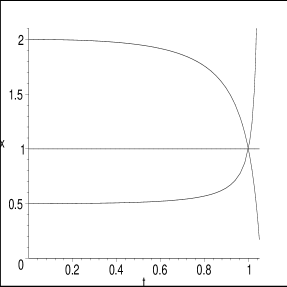
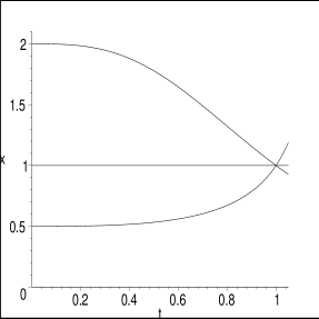
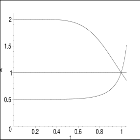
Figure 5: Left picture shows $x(t)$ as given by eq.(5.18) at different values of parameters: $b_{1}=1$, $b_{2}=-0.1$ (upper line), $b_{1}=\infty$, $b_{2}=0$ (middle line) and $b_{1}=-2$, $b_{2}=0.1$ (lower line). At $t<0.7-0.8$ this $x(t)$ behaves as $x(t)=const=\frac{b_{1}+1}{b_{1}}$, i.e. $2$, $1$ and $\frac{1}{2}$ respectively and satisfies equation of motion $\dot{x}=0$. In the vicinity of $t=1$, however, equation is violated so that $x(t)$ satisfies the boundary condition $x(1)=1$ instead. The size of the deviation domain is regulated by $b_{2}$: the smaller $b_{2}$ the smaller the region of deviation – and the more drastic is jump of $x(t)$ from exact solution to the boundary condition. The true solution $x(t)=1$ – which satisfies both equation of motion and boundary condition – is the only one which behaves smoothly under the variation of $b_{2}$. The two other pictures show the same phenomenon for eq.(5.20), for different number of iterations, $N=3$ (middle picture) and $N=6$ (right picture), and for different values of the free parameter, $x_{0}=2$ (upper line), $x_{0}=1$ (middle line) and $x_{0}=1\over 2$ (lower line). Again, the true solution with $x_{0}=1$ is distinguished by smooth dependence on the iteration number $N$. The difference with example in the left picture is that $x(t)$ is non-singular even beyond the segment $t=[0,1]$, instead $B(t)$ develops singularity at $t=1$.

One can also analyze other toy examples, which can be closer to realistic boundary rings. It can make sense to substitute (5.10) say, by

$$\begin{array}[]{c}x=t+x(1-t)B\end{array}$$ (5.19)

keeping in mind that $x$ models the ratio $y_{0}/y_{2}$ and $t$ models $y_{1}^{2}$, so that (5.19) resembles (5.2) at small $y_{2}$. Looking at this example one can see that exact solutions for $B(t)$ blow up at $t=1$, what is a slight additional complication, though it does not change our conclusions implied by analysis of (5.10). In particular, if exact $B(t)$ is substituted by its truncation at $N$-th level (i.e. if the first $N$ terms of $t$-expansion of $B(t)$ are kept), then the corresponding

$$\begin{array}[]{c}x_{N}(t)=\frac{x_{0}}{1+t^{N}(x_{0}-1)}\end{array}$$ (5.20)

and we see that the domain of deviation from exact solution $x=x_{0}$ is getting closer and closer to $t=1$ with increase of $N$. A typical behavior for $x_{0}\neq 1$ in the vicinity of the boundary $t=1$ has strong $N$-dependence, and the true solution $x=x_{0}=1$, which satisfies both the differential equation and boundary condition is distinguished by the lack of such $N$-dependence.

5.5 On continuation of solutions beyond $\Pi$

To further emphasize the difference between approximate solutions from s.4 and s.5, it deserves mentioning also that they have principally different behavior outside the polygon-bounded domain. Implication of (5.2) is that $r^{2}=P_{2}$ vanishes not only on $\Pi$ but also on all their continuations into the outside: on entire $n$ straight lines in $y$-space, which contain the $n$ segments of $\Pi$. This can easily be an artefact of polynomial-based consideration behind (5.2), which is not necessarily preserved in transition to functional analysis, like in s.4. On the other hand, solutions to Plateau problem in the flat Euclidean space are known to have this property [33]. Still, one should be cautious about this analogy, because in Euclidean case the basic equation is ordinary Laplace and minimal surfaces are too closely associated with complex analytic functions and the Schwarz reflection principle.

5.6 Recurrence relations for $b_{ij}^{(n)}$ from NG equations at $n=4$ and $n=6$

5.6.1 Relation between $b_{ij}$ and $c_{ij}$ at the level of generating functions

After providing some arguments in favor of (5.2) – and before showing impressive pictorial confirmation in s.5.7 below – we need to address the most difficult issue in this approach: solution of NG equations. In this paper we restrict ourselves to description of recurrence relations for coefficients of $B$ in (5.2) and to demonstration of one-to-one correspondence between $b$- and $c$-series from s.4.1. Problems of (uniform) convergence and theoretically-reliable approximation methods will be addressed elsewhere.

There are different possibilities to define a formal series for $B$, for example, one can take

$$\begin{array}[]{c}B=\sum_{i,j\geq 0}b_{ij}^{(n)}y_{0}^{2i}y^{2j}\end{array}$$ (5.21)

or, given the symmetries of the problem (in our $Z_{n}$-symmetric case),

$$\begin{array}[]{c}B=\sum_{i,j\geq 0}\tilde{b}_{ij}^{(n)}K_{n/2}^{2i}y^{2j}\end{array}$$ (5.22)

The advantage of the first representation is that it does not have explicit $n$-dependence and symmetry restrictions, however, these advantages can easily become disadvantages in particular numerical considerations (making calculations in symmetric situations more tedious than really needed), then the second representation can be used. In particular, with the second representation for $B$ eq.(5.2) is always (for all $n$) a cubic equation in $y_{0}$, what allows to formally rewrite it as analytical expression for $y_{0}(y_{1},y_{2})$ (despite based on low-efficient Cardano’s formulas, it drastically simplifies MAPLE calculations).

Substituting (5.21) into (5.2), we can solve for $y_{0}$ iteratively:

$$\begin{array}[]{c}y_{0}=\frac{K}{Q(y^{2})-(1-y_{1}^{2}-y_{2}^{2}+y_{0}^{2})B}=\frac{K(y_{1},y_{2})}{Q(y^{2})-(1-y^{2})B_{0}(y^{2})}+O(K^{3}),\end{array}$$ (5.23)

where

$$\begin{array}[]{c}B_{0}=\sum_{j\geq 0}b_{0j}y^{2j}=\sum_{j\geq 0}\tilde{b}_{0j}y^{2j}\end{array}$$ (5.24)

(obviously, at $i=0$ coefficients $\tilde{b}_{0j}=b_{0j}$). Comparing this to

$$\begin{array}[]{c}y_{0}=\sum_{ij}c_{ij}K^{2i+1}y^{2j}=K(y_{1},y_{2})Y_{0}(y^{2})+O(K^{3}),\ \ \ \ Y_{0}(y^{2})=\sum_{j\geq 0}c_{0j}y^{2j}\end{array}$$ (5.25)

we immediately obtain:

$$\begin{array}[]{c}Y_{0}(y^{2})=\frac{1}{Q(y^{2})-(1-y^{2})B_{0}(y^{2})}\end{array}$$ (5.26)

what provides a general expression for the coefficients $c_{0j}$ through $b_{0j}$ or – vice versa, of $b_{0j}$ through $c_{0j}$, if (5.26) is rewritten as

$$\begin{array}[]{c}B_{0}(y^{2})=\frac{Q(y^{2})Y_{0}(y^{2})-1}{(1-y^{2})Y_{0}(y^{2})}\end{array}$$ (5.27)

For example,

$$\begin{array}[]{c}c_{00}=\frac{1}{1-b_{00}},\\ c_{01}=\frac{\frac{n-4}{8}+b_{01}-b_{00}}{(1-b_{00})^{2}},\\ \ldots\end{array}$$

and

$$\begin{array}[]{c}b_{00}=\frac{c_{00}-1}{c_{00}},\\ b_{01}=\frac{12-n}{8}+\frac{c_{01}-c_{00}}{c_{00}^{2}},\\ \ldots\end{array}$$

This demonstrates that we indeed get a one-to-one relation, but when expressed in terms of generating functions, it is an equation with singularities at finite points, what signals about existence of potential convergence problems.

It is easy to find in a similar way the relations between generating functions $Y_{i}(y^{2})$ and $B_{i}(y^{2})$ (note that for $i\geq 1$ $\tilde{B}_{i}(y^{2})$ differs from $B_{i}(y^{2})$ – by an easily derived relation). However, we can also proceed in a more primitive way: substitute (5.21) into NG equation and obtain recurrence relations for $b_{ij}$ – just in the same way as we did for $c_{ij}$ in s.4.1. As in that case these relations depend on $n$, and we list the first few for $n=4$ and $n=6$. We give also explicit examples of triangular invertible relations between individual $b_{ij}^{(n)}$ and $c_{ij}^{(n)}$. Like above, index $n$ is often omitted to avoid further overloading of formulas.

5.6.2 $n=4$. Recurrence relations

$$\begin{array}[]{c}b_{01}=\frac{\big{(}4-5b_{00}\big{)}b_{00}}{6(1-b_{00})},\\ b_{02}=\frac{\big{(}63-262b_{00}+316b_{00}^{2}-115b_{00}^{3}\big{)}b_{00}}{144(1-b_{00})^{3}}-\frac{3b_{10}}{18(1-b_{00})^{2}},\\ b_{03}=\frac{\big{(}1188-9138b_{00}+23969b_{00}^{2}-28626b_{00}^{3}+15990b_{00}^{4}-3385b_{00}^{5}\big{)}b_{00}}{4320(1-b_{00})^{5}}-\\ -\frac{\big{(}84-178b_{00}+89b_{00}^{2}\big{)}b_{10}}{480(1-b_{00})^{4}}-\frac{3b_{11}}{10(1-b_{00})^{2}},\\ \ldots\\ b_{11}=-\frac{\big{(}3-86b_{00}+137b_{00}^{2}-53b_{00}^{3}\big{)}b_{00}}{126(1-b_{00})^{3}}+\frac{\big{(}69-118b_{00}+59b_{00}^{2}\big{)}b_{10}}{42(1-b_{00})^{2}}\\ \ldots\end{array}$$

These relations express all $b_{ij}$ in terms of the free parameters $b_{i0}$, which are not fixed by NG equations and boundary conditions. At $n=4$ they admit a solution $b_{ij}=0$, corresponding to $c_{ij}=\delta_{i1}\delta_{j1}$, i.e. to Alday-Maldacena square solution $y_{0}=y_{1}y_{2}$, see s.2.5 above. However, $b_{ij}^{(n)}=0$ will not be a solution at higher $n\geq 6$. The limit $c^{(n)}_{ij}=0$, leading to the $n=\infty$ solution (2.8.1) with a unit-circle boundary from the $Z_{n}$-symmetric ansatz, looks complicated in $b$-variables, even at $n=4$.

5.6.3 $n=6$. Recurrence relations for $b_{ij}$

Similarly, for $n=6$ we get:

$$\begin{array}[]{c}b_{01}=\frac{1+5b_{00}}{8},\\ b_{02}=\frac{28+130b_{00}-185b_{00}^{2}}{80(1-b_{00})},\\ b_{03}=\frac{35+127b_{00}-471b_{00}^{2}+285b_{00}^{3}-24b_{10}}{512(1-b_{00})^{2}},\\ b_{04}=\frac{38284+93700b_{00}-766310b_{00}^{2}+1022700b_{00}^{3}-390075b_{00}^{4}}{716800(1-b_{00})^{3}}+\frac{123b_{10}}{1280(1-b_{00})^{2}},\\ b_{05}=\frac{5204441+5826459b_{00}-136463910b_{00}^{2}+301180330b_{00}^{3}-243508650b_{00}^{4}+67625250b_{00}^{5}}{126156800(1-b_{00}^{4})}-\\ -\frac{3\big{(}10630-21098b_{00}+10549b_{00}^{2}\big{)}b_{10}}{225280(1-b_{00})^{4}},\\ \ldots\\ b_{11}=\frac{28-290b_{00}+505b_{00}^{2}}{1600(1-b_{00})}+\frac{13b_{10}}{10},\\ b_{12}=\frac{249-18609b_{00}+73260b_{00}^{2}-47740b_{00}^{3}}{70400(1-b_{00})^{2}}+\frac{\big{(}2840-5302b_{00}+2651b_{00}^{2}\big{)}b_{10}}{1760(1-b_{00})^{2}},\\ \ldots\end{array}$$

These formulas express all $b_{ij}$ in terms of the free parameters (moduli) $b_{i0}$, which are not immediately fixed by NG equations and the boundary conditions. As explained in [4, 23] these moduli (whenever they exist) are not necessarily inessential in consideration of $\epsilon$-regularized NG actions (areas) in the study of Alday-Maldacena program. As also explained in these papers, there are two ways to deal with such moduli: either understand their raison d’etre and eliminate in a rigorous way (say, using Virasoro constraints in the case of [4, 23], or analysis from s.5.4 in our present situation) – what can be quite a tedious thing to do,– or simply minimize the answer, i.e. regularized area, w.r.t. the variation of moduli – this can be a simpler thing to do in practice and, even more important, this can also reveal some additional hidden structures behind our problem (like the height function in [4, 23]).

5.6.4 $n=6$: Relation between $b_{ij}$ and $c_{ij}$

As a simple example of this relation we present a few first formulas for $n=6$. The first two lines coincide with (5.6.1).

$$\begin{array}[]{c}c_{00}=\frac{1}{1-b_{00}},\\ c_{01}=\frac{(1-4b_{00}+4b_{01})}{4(1-b_{00})^{2}}=\frac{(1-4b_{00})}{4(1-b_{00})^{2}}+\frac{b_{01}}{(1-b_{00})^{2}},\\ c_{02}=\frac{(1-4b_{00})^{2}}{16(1-b_{00})^{3}}-\frac{(1+2b_{00}-4b_{01})b_{01}}{16(1-b_{00})^{3}}+\frac{b_{02}}{(1-b_{00})^{2}},\\ c_{03}=\frac{(1-4b_{00})^{3}}{64(1-b_{00})^{4}}-\frac{(5+4b_{00})(1-4b_{00}+4b_{01})b_{01}}{16(1-b_{00})^{4}}+\frac{b_{01}^{3}}{(1-b_{00})^{4}}-\frac{(1+2b_{00}-4b_{01})b_{02}}{2(1-b_{00})^{3}}+\frac{b_{03}}{(1-b_{00})^{2}},\\ \ldots\\ \\ c_{10}=\frac{b_{00}+b_{10}}{(1-b_{00})^{4}},\\ \ldots\end{array}$$

5.7 Approximate NG solutions with exact boundary conditions

Thus, one is finally prepared for the final set of examples. Similarly to s.4.4, one can build a set of plots in order to see how the approximation works.. The difference is that now one has to use

$$\begin{array}[]{c}y_{0}=\frac{K_{3}}{1-\frac{y^{2}}{4}}\end{array}$$ (5.28)

instead of (4.25) and

$$\begin{array}[]{c}y_{0}=\frac{K_{3}}{1-\frac{y^{2}}{4}-(1+y_{0}^{2}-y^{2})b_{00}}\end{array}$$ (5.29)

instead of (4.26). Similar modifications has to be made for other values of $n$. Note that the r.h.s. of (5.28) can not be multiplied by any constant without breaking (5.2): coefficient at the r.h.s. is strictly unity. As to (5.29), it contains a free parameter $b_{0}$, but equation still needs to be resolved w.r.t. $y_{0}$ (actually, this is a cubic equation).

In this case, any plot confirms that the boundary conditions are exactly satisfied – what looks impressive after comparison with the results of s.4. Moreover, in accordance with expectations of s.5.5, matching extends to entire straight lines, beyond $\Pi$ itself. Unfortunately, we did not yet invent an equally nice visualization of deviations from the NG equations – which, as we discussed, can be strong in the vicinity of the boundary $\Pi$, unless the remaining free parameters (like $b_{00}$) are adjusted to some unique true value. Therefore, it remains unclear whether this type of criterium can be effective for the practical search of these true values. Still even the very rough approximation like (5.28) can already be applied to the study of string/gauge duality. The next step to be made is evaluation of regularized areas for configurations like (5.28).

6 Conclusion

In this paper we discussed a systematic approach to construction of NG solutions in AdS backgrounds with polygons, consisting of null vectors, in the role of bounding contour at infinity.

It is suggested to look for NG solutions in the form of formal series, restricted by symmetries (if any) and boundary conditions. Boundary conditions can be explicitly taken into account by expanding formal-series in elements of the boundary ring, which consists of all polynomials vanishing at the boundary polygon. NG equations provide recurrence relations for the coefficients of formal series.

Actually, boundary conditions can be imposed on formal series both before and after their substitution into NG equations.

While the first options (it is considered in s.5) seems to be conceptually and aesthetically better, it does not provide immediate practical way to fix the remaining free parameters from the first principles. For application purposes this is not obligatory a problem, because approximately evaluated regularized area can be simply minimized w.r.t. to such parameters – resembling the way the $z$-variables have been handled in [4].

The second option (considered in s.4) is less attractive, instead it produces spectacularly accurate approximations to the would-be exact solutions, and even the boundary conditions seem to be matched pretty well. Inaccuracies seem to increase in the vicinities of the polygon angles, which give dominant contributions to the IR divergencies of regularized areas. This is one of the problems which should be addressed when one tries to make use of these methods in the further studies of string/gauge dualities. Note that this problem (at least at the level of quadratic divergencies) is a priori avoided if the first option is chosen, because boundary conditions are imposed exactly.

To conclude, our concrete suggestion for further development of Alday-Maldacena program is to take the $B=0$ version of (5.2), i.e.

$$\begin{array}[]{c}y_{0}=\frac{K_{n/2}}{Q_{(n)}(y^{2})}\,,\\ r=\sqrt{y_{0}^{2}+1-y_{1}^{2}-y_{2}^{2}}\end{array}$$

as the first approximation to the minimal surface, and concentrate on developing technique for evaluating regularized areas for such surfaces (see table in s.3.3.5 for a list of $K_{n/2}$ and $Q_{(n)}$). After this is done, one can begin including corrections to (6), implied by NG equations, which can be systematically found by the methods of the present paper. NG equations fix functional form ($y_{1}$ and $y_{2}$ dependence) of corrections in any given order, and remaining free parameters can be fixed by the general method of [4]: by extremizing the resulting integral (see also comments at the end of s.5.6.3). Generalization of (6) beyond the $Z_{n}$-symmetric polygons $\Pi$ will be considered elsewhere.

References

- [1] Z.Bern, L.Dixon and V.Smirnov, Iteration of Planar Amplitudes in Maximally Supersymmetric Yang-Mills Theory at Three Loops and Beyond, Phys.Rev. D72 (2005) 085001, hep-th/0505205
-
[2]
L.Lipatov, Evolution Equations in CQD, ICTP
Conference, May, 1997
J.Minahan and K.Zarembo, The Bethe-Ansatz for N=4 Super Yang-Mills, JHEP 0303 (2003) 013, hep-th/0212208
N.Beisert, C.Kristjansen and M.Staudacher, The Dilatation Operator of Conformal N=4 Super Yang-Mills Theory, Nucl.Phys. B664 (2003) 131-184, hep-th/0303060
N.Beisert, B.Eden and M.Staudacher, Transcendentality and Crossing, J.Stat.Mech. 0701 (2007) P021, hep-th/0610251
M.Staudacher, Dressing, Nesting and Wrapping in AdS/CFT, Lecture at RMP Workshop, Copenhagen, 2007 - [3] A.Brandhuber, P.Heslop and G.Travaglini, MHV Aplitudes in Super Yang-Mills and Wilson Loops, arXiv:0707.1153
- [4] A.Mironov, A.Morozov and T.N.Tomaras, On n-point Amplitudes in N=4 SYM, JHEP 11 (2007) 021, arXiv:0708.1625
- [5] L.Alday and J.Maldacena, Gluon Scattering Amplitudes at Strong Coupling, arXiv:0705.0303
- [6] S.Abel, S.Forste and V.Khose, Scattering Amplitudes in Strongly Coupled SYM from Semiclassical Strings in AdS, arXiv:0705.2113
- [7] E.Buchbinder, Infrared Limit of Gluon Amplitudes at Strong Coupling, arXiv:0706.2015
- [8] J.Drummond, G.Korchemsky and E.Sokatchev, Conformal properties of four-gluon planar amplitudes and Wilson loops, arXiv:0707.0243
- [9] F.Cachazo, M.Spradlin and A.Volovich, Four-Loop Collinear Anomalous Dimension in N = 4 Yang-MillsTheory, arXiv:0707.1903
- [10] M.Kruczenski, R.Roiban, A.Tirziu and A.Tseytlin, Strong-Coupling Expansion of Cusp Anomaly and Gluon Amplitudes from Quantum Open Strings in , arXiv:0707.4254
- [11] Z.Komargodsky and S.Razamat, Planar Quark Scattering at Strong Coupling and Universality, arXiv:0707.4367
- [12] L.Alday and J.Maldacena, Comments on Operators with Large Spin, arXiv:0708.0672; Comments on gluon scattering amplitudes via AdS/CFT, arXiv:0710.1060
- [13] A.Jevicki, C.Kalousios, M.Spradlin and A.Volovich, Dressing the Giant Gluon, arXiv:0708.0818
- [14] A.Mironov, A.Morozov and T.N.Tomaras, On n-point Amplitudes in N=4 SYM, arXiv:0708.1625
- [15] H.Kawai and T.Suyama, Some Implications of Perturbative Approach to AdS/CFT Correspondence, arXiv:0708.2463
- [16] S.G.Naculich and H.J.Schnitzer, Regge behavior of gluon scattering amplitudes in N=4 SYM theory, arXiv:0708.3069
- [17] R.Roiban and A.A.Tseytlin, Strong-coupling expansion of cusp anomaly from quantum superstring, arXiv:0709.0681
- [18] J.M.Drummond, J.Henn, G.P.Korchemsky and E.Sokatchev, On planar gluon amplitudes/Wilson loops duality, arXiv:0709.2368
- [19] D.Nguyen, M.Spradlin and A.Volovich, New Dual Conformally Invariant Off-Shell Integrals, arXiv:0709.4665
- [20] J.McGreevy and A.Sever, Quark scattering amplitudes at strong coupling, arXiv:0710.0393
- [21] S.Ryang, Conformal SO(2,4) Transformations of the One-Cusp Wilson Loop Surface, arXiv:0710.1673
- [22] D.Astefanesei, S.Dobashi, K.Ito and H.S.Nastase, Comments on gluon 6-point scattering amplitudes in N=4 SYM at strong coupling, arXiv:0710.1684
- [23] A.Mironov, A.Morozov and T.Tomaras, Some properties of the Alday-Maldacena minimum, arXiV:0711.0192 (hep-th), to appear in Physics Letters B
- [24] A.Popolitov, On coincidence of Alday-Maldacena-regularized -model and Nambu-Goto areas of minimal surfaces, arXiv:0710.2073
- [25] Gang Yang, Comment on the Alday-Maldacena solution in calculating scattering amplitude via AdS/CFT, arXiv:0711.2828
- [26] K.Ito, H.S.Nastase and K.Iwasaki, Gluon scattering in Super Yang-Mills at finite temperature, arXiv:0711.3532
- [27] R.Kallosh and A.Tseytlin, Simplifying Superstring Action on , JHEP 9810 (1998) 016, hep-th/9808088
-
[28]
N.Drukker, D.Gross and H.Ooguri,
Wilson Loops and Minimal Surfaces, Phys.Rev. D60 (1999)
125006, hep-th/9904191
Yu.Makeenko,Light-Cone Wilson Loops and the String/Gauge Correspondence, JHEP 0301 (2003) 007, hep-th/0210256 - [29] M.Kruczenski, A Note on Twist Two Operators in SYM and Wilson Loops in Minkowski Signature, JHEP 0212 (2002) 024, hep-th/0212115
-
[30]
A.Kotikov, L.Lipatov and V.Velizhanin,
Anomalous Dimensions of Wilson Operators in
SYM Theory, Phys.Lett. B557 (2003) 114-120, hep-ph/0301021
A.Kotikov, L.Lipatov, A.Onishchenko and V.Velizhanin, Three-Loop Universal Anomalous Dimension of the Wilson Operators in SUSY Yang-Mills Model, Phys.Lett. B595 (2004) 521-529; Erratum-ibid. B632 (2006) 754-756, hep-th/0404092 -
[31]
For modernized presentation of the subject see
V.Dolotin and A.Morozov, The Universal Mandelbrot Set, Beginning of the Story, World Scientific, 2006; hep-th/0501235; hep-th/0701234;
Andrey Morozov, JETP Letters, 86, N11 (2007); arXiv:0710.2315
V.Dolotin and A.Morozov, Introduction to non-linear Algebra, World Scientific, 2007; hep-th/0609022;
Sh.Shakirov, Theor.Math.Phys., 153(2) (2007) 1477-1486; math/0609524
For traditional textbooks see
S.Lang, Algebra, Addison-Wesley Seires in Mathematics, 1965
B.L.Van der Varden, Algebra, I, II, Springer-Verlag, 1967, 1971 - [32] A.Morozov and M.Serbyn, Theor.Math.Phys., to appear, hep-th/0703258
-
[33]
See discussion of Schwarz reflection
principle at the bottom of page 16 of English edition or at
page 28 of Russian edition in
P.Hoffman and H.Karcher, Complete Embedded Minimal Surfaces of Finite Total Curvature, in Encyclopaedia of Math.Science, 90, Geometry V. Minimal Surfaces, ed.R.Osserman, Springer