Magnetic Complexity in Eruptive Solar Active Regions and Associated Eruption Parameters

Abstract

Using an efficient magnetic complexity index in the active-region solar photosphere, we quantify the preflare strength of the photospheric magnetic polarity inversion lines in 23 eruptive active regions with flare/CME/ICME events tracked all the way from the Sun to the Earth. We find that active regions with more intense polarity inversion lines host statistically stronger flares and faster, more impulsively accelerated, CMEs. No significant correlation is found between the strength of the inversion lines and the flare soft X-ray rise times, the ICME transit times, and the peak $D_{st}$ indices of the induced geomagnetic storms. Corroborating these and previous results, we speculate on a possible interpretation for the connection between source active regions, flares, and CMEs. Further work is needed to validate this concept and uncover its physical details.

GEORGOULIS MAGNETIC COMPLEXITY AND ERUPTIVE ACTIVITY IN THE SUN Manolis K. Georgoulis, The Johns Hopkins University Applied Physics Laboratory, 11100 Johns Hopkins Rd., Laurel, MD 20723, USA. (manolis.georgoulis@jhuapl.edu)

Gindraft=false

1 Introduction

The Solar and Heliospheric Observatory (SoHO) has established coronal mass ejections (CMEs) as an integral part of solar eruptions. Today we know that there exist slow and fast CMEs associated with eruptive quiet-Sun filaments and solar flares, respectively, with a wide velocity distribution ranging between a few tens of $km/s$ to $\sim 3000\;km/s$ (St. Cyr et al. 2000; Yashiro et al. 2004; Yurchyshyn et al. 2005). Solar flares are an exclusive characteristic of solar active regions (ARs), so fast CMEs, typically with velocities $\geq 750\;km/s$, are active-region CMEs (Sheeley et al. 1999). Furthermore, the soft X-ray rise phase of the eruptive flares almost coincides with the main acceleration phase of the resulting CMEs (Zhang et al. 2001; Zhang and Dere 2006).

Observations and models have been utilized to relate specific AR characteristics with CME speeds. Following a “big AR syndrome”, extraordinary ARs can trigger superfast CMEs (Gopalswamy et al. 2005), but a more quantitative connection is lacking. Only recently, Qiu and Yurchyshyn (2005) reported a strong correlation between CME speeds and the reconnected magnetic flux in two-ribbon flares, Su et al. (2007) combined magnetic flux and shear to improve correlations with flare magnitudes and CME speeds, and Török and Kliem (2007) concluded that increased magnetic complexity, reflected on steep magnetic gradients in the source ARs’ corona, tends to produce faster CMEs.

The above studies suggest that complex (multipolar and/or with pronounced magnetic polarity inversion lines [PILs]) ARs tend to produce faster CMEs. Here, we investigate this effect further, reporting on work done in the framework of the Living With a Star Coordinated Data Analysis Workshops (LWS/CDAW). We identified 23 source ARs with eruptions unambiguously traced from the solar surface to 1 AU. For these ARs, we correlate the peak photospheric complexity prior to an eruption with various eruption parameters, including flare magnitudes, plane-of-sky CME velocities, and (assumed constant) CME acceleration magnitudes. Our analysis involves full-halo CMEs with source ARs located close to disk center. Therefore, it should be kept in mind that significant discrepancies may exist between the measured (plane-of-sky) and the true (unprojected) CME velocities (Schwenn et al. 2005), that may have an impact on correlations. For this and other reasons, as discussed below, we emphasize the statistical aspect of the reported correlations, trying to avoid strong quantitative conclusions.

2 Magnetic Complexity Analysis and Data Selection

Georgoulis and Rust (2007) defined the effective connected magnetic field strength, $B_{eff}$, that characterizes a given AR at a given time. The larger the value of $B_{eff}$, the more intense the PIL(s) present in the AR. The intensity of a PIL increases when massive amounts of bipolar magnetic flux are tightly concentrated around it. To calculate $B_{eff}$ for the $p$ positive-polarity and $n$ negative-polarity flux concentrations that comprise an AR, we calculate two $p\times n$ connectivity matrices: $\Phi_{i,j}$, containing the magnetic fluxes that connect a positive-polarity concentration $i$ ($i\in[1,p]$) to a negative-polarity concentration $j$ ($j\in[1,n]$), and $L_{i,j}$, containing the respective separation lengths of the connections. Then, $B_{eff}$ is the sum of all finite elements $(\Phi_{i,j}/L_{i,j}^{2})$.

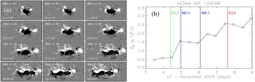
Figure 1: Photospheric evolution in NOAA AR 10696 over a period of 6 days in 2004 November. (a) Normal photospheric magnetic field in the AR. Notice the gradual enhancement of the PIL’s strength and spatial extent. Tic mark separation in all images is $10$” ($\sim 7250\;km$ in the solar photosphere). Solar north is up; west is to the right. (b) Timeseries of the respective $B_{eff}$-values. Notice the repeated flaring activity (onset times indicated by the color lines) as $B_{eff}$ increases.

Georgoulis and Rust (2007) calculated $B_{eff}$ for $\sim 2140$ SoHO/MDI magnetograms corresponding to 298 ARs. To avoid severe projection effects, each AR was required to be located within $41^{o}$ EW from solar disk center. Each AR needed 6-7 days to traverse this $82^{o}$-zone, and this determined the typical observing period. To further account for projection effects, we (i) estimated the normal AR magnetic field by dividing the line-of-sight field by $cos\theta$, where $\theta$ is the angular distance of each location from disk center, (ii) constructed the local, heliographic, plane, and (iii) interpolated the normal field on the heliographic plane. We found that $B_{eff}$ efficiently distinguishes eruptive from non-eruptive ARs and that a well-defined probability for major (X- and M-class, although not their exact magnitudes) flares depends solely on $B_{eff}$. An example of how an increase in $B_{eff}$ translates to stronger PILs that, in turn, give rise to repeated flaring activity, is shown in Figure 1.

Zhang et al. (2007), on the other hand, identified the solar sources of 88 geoeffective ($D_{st}\leq-100\;nT$) solar eruptions. Each of these eruptions was traced from solar source to geomagnetic effect. An AR source could be identified for 54 of the above 88 events, with 23 different source ARs present.

Combining the above two works, we calculated the peak pre-eruption (12 hr, at most, before each flare’s onset) $B_{eff}$-values for these 23 source ARs. The AR and eruption data are summarized in Table 1.

3 Results

We seek a possible link between the peak AR photospheric complexity, quantified by the peak $B_{eff}$, and the flare magnitude or CME kinematics. The flare magnitudes are related to the peak preflare $B_{eff}$-values in Figure 2a. To calculate the logarithmic flare magnitude we arbitrarily assign a magnitude of 1 to a C1.0 flare. This implies a magnitude of 10, 100, and 1000, for a M1.0, X1.0, and X10, flares, respectively (dashed lines). Notice the significant correlation coefficients (cc) between the flare magnitude and $B_{eff}$, despite the scatter. The correlation clearly implies an increasing flare magnitude for an increasing preflare $B_{eff}$. However, predictions of the flare magnitude using the shown scaling are not recommended. This is because an AR may not yield its strongest flare within the typical 6-7 day observing period despite showing a high (close to peak) $B_{eff}$-value. The scatter in Figure 2a might also highlight the probabilistic (or even stochastic) nature of flare triggering, with the flare magnitude depending in part on the local magnetic conditions and their synergy. The goodness of fit in Figure 2a has a confidence level of $\sim 98.6$%. In brief, increasing $B_{eff}$ in an AR statistically implies stronger flares triggered in the AR.

In Figure 2b we correlate the plane-of-sky CME velocities $V_{CME}$ with the peak preflare $B_{eff}$-values. Although the small dynamical range of $V_{CME}$ gives rise to lower and more fragile correlation coefficients, the scatter around the least-squares best fit appears smaller in this case. This allows the introduction of a scaling relation between $V_{CME}$ and peak preflare $B_{eff}$ that reads

$$V_{CME}(km/s)\simeq 87.3\times B_{eff}^{0.38\pm 0.12}(G)\;\;.$$ (1)

Equation (1) is, again, not recommended for accurate predictions of $V_{CME}$ but it suggests that more complex ARs, with larger and more intense PILs, statistically give rise to faster CMEs. For the smallest considered $B_{eff}$-value ($\sim 500\;G$) we anticipate $V_{CME}\simeq 920\;km/s$, in good agreement with the slower end of AR CMEs ($\sim 750\;km/s$). For our largest $B_{eff}$ ($\sim 5000\;G$), we expect $V_{CME}\simeq 2200\;km/s$, that is relatively close to (but somewhat smaller than) the largest measured CME velocities ($\sim 2800\;km/s$). The difference between the two extreme velocities is $\sim 21$%, with a typical $\sim 10$%-uncertainty for the measured plane-of-sky CME speed (J. Zhang, private communication). The goodness of fit in Figure 2b has a confidence level of $\sim 91$%. Therefore, it is clear that increasing $B_{eff}$ in an AR statistically implies faster CMEs triggered in the AR.

In Figure 2c we correlate the CME acceleration magnitude $\gamma_{CME}$ with the peak preflare $B_{eff}$. We have estimated a constant $\gamma_{CME}$ by the ratio $(V_{CME}/T_{flare})$, i.e., by following the “flare-proxy” approach (Zhang and Dere 2006) implying that $T_{flare}$ also reflects the main CME acceleration phase. Although the trend in Figure 2c is to attain stronger $\gamma_{CME}$ with increasing $B_{eff}$, the correlation is not as appreciable as in Figures 2a, 2b. The goodness of the fit is also lower (confidence level $\sim 80$%). Besides numerical effects (e.g., discrepancies between plane-of-sky and true CME velocity), the weaker correlation between $\gamma_{CME}$ and $B_{eff}$ may be due to (i) the assumption of a constant CME acceleration magnitude, and/or (ii) the very weak anti-correlation between $T_{flare}$ and $B_{eff}$ (cc $\in(-0.14,-0.18)$ - not shown). The loose association between $T_{flare}$ and $B_{eff}$ means that the intensity of PILs in ARs correlates only weakly with the impulsiveness of the flares triggered in these ARs. Nevertheless, Figure 2c suggests that increasing $B_{eff}$ in an AR statistically implies more impulsively accelerated CMEs triggered in the AR.

We did not find significant correlations (maximum cc $\in(0.2,0.5)$ and maximum confidence levels $\sim 70$%) when correlating $B_{eff}$ with (i) the ICME transit time $T_{ICME}$ and (ii) the peak absolute $D_{st}$ index of the resulting geomagnetic storms. Neither result is surprising: Schwenn et al. (2005) and Manoharan (2006) report some correlation between $T_{ICME}$ and $V_{CME}$ but with substantial scatter. Other heliospheric effects may also impact the velocity profile , and hence the arrival time, of ICMEs (Chen 1996; Cargill 2004; Tappin 2006). Regarding $D_{st}$, many factors, besides the source AR’s complexity, affect the ICME geoeffectiveness. These factors include, but are not limited to, the CME’s source location in the solar disk, the orientation of the possible post-eruption flux rope, in-situ heliospheric distortions, turbulence, interactions with other heliospheric transients, and the ICME velocity profile.

4 Conclusions and Discussion

In a previous work (Georgoulis and Rust 2007) we quantified the photospheric magnetic complexity in solar ARs, where complexity reflects the strength of PILs in these ARs. In this work we combined our sample of ARs with the sample of AR sources that triggered major geomagnetic eruptions (Zhang et al. 2007). We identified 23 source ARs for which we have preflare AR magnetograms, and we correlated the peak pre-eruption AR complexity with various eruption parameters.

Significant correlations were uncovered when plotting the peak value of the AR complexity index, $B_{eff}$, vs. (from stronger to weaker correlation) (i) the flare magnitude, (ii) the CME velocity, and (iii) an assumed constant CME acceleration magnitude. Though not ideal for predictive purposes, these correlations clearly imply that more complex ARs, with intense PILs, can produce statistically stronger flares and faster, more impulsively accelerated, CMEs. Our finding goes a step further than the usual “big AR syndrome”: big (flux-massive) ARs are not necessarily ARs with intense PILs, and hence with large $B_{eff}$-values, although the opposite is almost always true.

At this point, we can only speculate on a possible interpretation of our results, making it clear that only further work can validate or rule out our scenario. Given that the main CME acceleration phase nearly coincides with the flare impulsive phase, the initial ascending structure evolving into a CME (hereafter CME precursor) should start expanding before the flare. As it expands, the CME precursor interacts with the surrounding PIL-supported magnetic structure causing magnetic reconnection. Reconnection in stronger magnetic fields organized along more intense PILs statistically leads to stronger flares (Figure 2a). Stronger flares imply larger amounts of released magnetic energy that, in turn, probably destabilize larger parts of the PIL-sustained structure and/or accelerate the unstable magnetic fields to higher speeds, thus giving rise to statistically faster (Figure 2b) and more impulsive (Figure 2c) CMEs. Again, the above indicate only statistical trends - the local field conditions at the flare location along the PIL as well as the overlaying solar magnetic fields (steep magnetic gradients [Török and Kliem 2007], coronal null points [Antiochos et al. 1999], etc.) affect both flare magnitudes and CME velocity profiles. Sometimes, fast CMEs are associated with relatively weak flares or vice-versa (Vršnak et al. 2005).

The above idea might also help understand the difference between (i) confined and eruptive flares and (ii) fast active-region CMEs and slow quiet-Sun CMEs. In case the PIL-supported structure, despite the reconnection, survives the perturbation applied by the CME precursor, a confined flare occurs. If there is no intense PIL, the CME precursor might easily destabilize the surrounding magnetic structure (especially in the presence of “open” overlaying fields, such as a streamer in the high corona) but, since only minor reconnection is expected, no major flare and a rather slow CME will occur. This might be the case for some quiet-Sun CMEs.

While our statistical results appear solid, only further work can validate the above physical scenario. It would be essential to (i) uncover the physical mechanism(s) responsible for the possible CME precursor (e.g., small-scale helical kink instability, magnetic flux cancellation on the PIL, etc.), and (ii) find the relation between the plane-of-sky velocity $V_{CME}$ and the true CME velocity and determine whether this improves the correlation with $B_{eff}$ or the source AR’s complexity in general. The Solar Terrestrial Relations Observatory (STEREO) can be instrumental in revealing the true CME velocities to be used for definitive conclusions in our quest to understand the erupting Sun.

Table 1: Summary of the 23 LWS/CDAW events used in our study, where the peak preflare $B_{eff}$-value of the source ARs and the corresponding eruptions are selected. Shown are the date and UT time of the flare onset, the flare class, the soft X-ray flare rise time ($T_{flare}$), the plane-of-sky CME velocity ($V_{CME}$), the CME acceleration magnitude ($\gamma_{CME})$, the ICME transit time ($T_{ICME}$ - n/a means that $T_{ICME}$ could not be calculated), the peak $D_{st}$ index, the NOAA AR number, and the peak $B_{eff}$-value.

	Flare				CME		ICME		Source
Event	Date	Onset	Class	$T_{flare}$	$V_{CME}$	$\gamma_{CME}$a	$T_{ICME}$b	$D_{st}$	NOAA	$B_{eff}$
		(UT)		($min$)	($km/s$)	($m/s^{2}$)	($hr$)	($nT$)	AR #	($G$)
1	11/04/97	06:10	X2.1	6	785	2181	45.8	-110	8100	1521.95
2	05/02/98	14:06	X1.1	11	938	1421	n/a	-205	8210	790.21
3	11/05/98	20:44	M8.4	55	523	158	79.3	-142	8375	958.02
4	02/10/00	02:30	C7.3	28	944	562	54.5	-133	8858	1323.7
5	07/14/00	10:54	X5.7	21	1674	1329	32.1	-301	9077	1741.6
6	09/16/00	05:18	M5.9	20	1215	1013	39.7	-201	9165	1108.7
7	10/09/00	23:50	C6.7	24	798	554	84.2	-107	9182	873.81
8	11/26/00	17:06	X4.0	14	980	1167	46.9	-119	9236	898.88
9	03/29/01	10:26	X1.7	18	942	872	42.6	-387	9393	3985.6
10	04/10/01	05:30	X2.3	20	2411	2009	40.5	-271	9415	1806.0
11	09/24/01	10:30	X2.6	66	2402	607	n/a	-102	9632	1265.2
12	10/19/01	16:50	X1.6	17	901	883	51.2	-187	9661	937.13
13	10/25/01	15:26	X1.3	20	1092	910	n/a	-157	9672	1289.4
14	11/04/01	16:35	X1.0	17	1810	1775	44.4	-292	9684	1324.1
15	04/17/02	08:26	M2.6	38	1240	544	63.6	-149	9906	774.56
16	08/16/02	12:30	M5.2	60	1585	440	98.5	-106	10069	2638.7
17	05/28/03	00:50	X3.6	10	1366	2277	36.2	-144	10365	2162.4
18	10/29/03	20:54	X10.	12	2029	2818	29.1	-383	10486	4338.1
19	11/18/03	08:50	M3.9	19	1660	1456	49.2	-422	10501	1183.5
20	07/20/04	13:31	M8.6	10	710	1183	52.5	-101	10652	1080.9
21	11/07/04	16:54	X2.0	24	1759	1222	51.1	-289	10696	2552.7
22	01/15/05	23:06	X2.6	37	2861	1289	n/a	-121	10720	2327.0
23	05/13/05	17:12	M8.0	44	1128	427	36.8	-263	10759	634.30

aThe CME acceleration magnitude is estimated by the ratio $(V_{CME}/T_{flare})$. bThe ICME transit time is calculated as the time difference between the ICME start time and the flare onset time

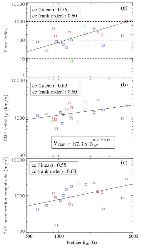
Figure 2: Correlation between the preflare $B_{eff}$-values and (a) the flare magnitude (the three dashed lines indicate, from low to high, M1.0, X1.0, and X10. flares), (b) the plane-of-sky CME velocity, and (c) the CME acceleration magnitude for the 23 events summarized in Table 1. In all plots, the straight lines indicate the least-squares best fit. C-, M-, and X-class flares are indicated by green, blue, and red squares, respectively. Both the Pearson (linear) and the Spearman (rank order) correlation coefficients (cc) are shown. For the correlation between $V_{CME}$ and $B_{eff}$ (b) the actual scaling formula is included in an inset.