Triaxial orbit based galaxy models with an application to the (apparent) decoupled core galaxy NGC 4365
Abstract
We present a flexible and efficient method to construct triaxial dynamical models of galaxies with a central black hole, using Schwarzschild’s orbital superposition approach. Our method is general and can deal with realistic luminosity distributions, which project to surface brightness distributions that may show position angle twists and ellipticity variations. The models are fit to measurements of the full line-of-sight velocity distribution (wherever available). We verify that our method is able to reproduce theoretical predictions of a three-integral triaxial Abel model. In a companion paper (van de Ven, de Zeeuw & van den Bosch), we demonstrate that the method recovers the phase-space distribution function. We apply our method to two-dimensional observations of the E3 galaxy NGC 4365, obtained with the integral-field spectrograph SAURON, and study its internal structure, showing that the observed kinematically decoupled core is not physically distinct from the main body and the inner region is close to oblate axisymmetric.
keywords:
galaxies: elliptical and lenticular, cD - galaxies: kinematics and dynamics - galaxies: structure1 Introduction
Binney (1976, 1978) argued convincingly that elliptical galaxies may well have triaxial intrinsic shapes, based on the observed slow rotation of the stars (Bertola & Capaccioli 1975; Illingworth 1977), the presence of isophote twists in the surface brightness distribution (e.g., Williams & Schwarzschild 1979), the presence of velocity gradients along the apparent minor axis (‘minor-axis rotation’, Schechter & Gunn 1978), and evidence from N-body simulations (Aarseth & Binney 1978). Schwarzschild’s (1979, 1982) numerical models demonstrated that such systems can be in dynamical equilibrium, and suggested that their observed kinematics can be rich (see also, e.g., Statler 1991). This is supported by the discovery of kinematically decoupled cores in the late nineteen-eighties (Bender 1988; Franx & Illingworth 1988) and, more recently, by observations with integral-field spectrographs such as SAURON, which reveal that some ellipticals have point-symmetric rather than bi-symmetric velocity fields, and often contain kinematically decoupled components (e.g., Emsellem et al. 2004). This means that these galaxies are not axisymmetric.
Subsequent work on triaxial dynamical models focused mostly on models with a cusp in the central density profile, on the effect of a central black hole, and on the range of shapes for which triaxial models could be in dynamical equilibrium (e.g., Gerhard & Binney 1985; Levison & Richstone 1987; Statler 1987; Hunter & de Zeeuw 1992; Schwarzschild 1993; Merritt & Fridman 1996; Siopis 1998; Terzić 2002). With the exception of studies of the Galactic Bulge (Zhao 1996; Häfner et al. 2000), most of this work was restricted to finding (numerical) distribution functions consistent with a given triaxial density. This showed that many different distribution functions may reproduce the same triaxial density, and that these dynamical models all have different observable kinematic properties, but detailed comparison to observations received little attention (Arnold, de Zeeuw & Hunter 1994; Mathieu & Dejonghe 1999). Ad-hoc kinematic models were used to constrain the distribution of intrinsic shapes (Binney 1985; Franx, Illingworth & de Zeeuw 1991) or of individual objects (Tenjes et al. 1993; Statler 1994b, 2001; Statler, Dejonghe & Smecker-Hane 1999; Statler et al. 2004).
The possibility to measure accurate line-of-sight velocity distributions (LOSVDs) in elliptical galaxies from observations of the stellar absorption lines (e.g., Bender 1990; van der Marel & Franx 1993), and the realization that these are the only way to distinguish radial variations in mass-to-light-ratio from radial variations in the anisotropy of the orbital structure (Dejonghe 1987; Gerhard 1993), led to the development of detailed spherical, and subsequently axisymmetric, numerical dynamical models aimed to fit all these kinematic measurements. These are generally constructed with a variant of Schwarzschild’s (1979) orbit superposition method, in which occupation numbers are found for a representative library of orbits calculated in the gravitational potential of the galaxy. The aim is to measure the mass of the central black holes (van der Marel et al. 1998; Gebhardt et al. 2003; Valluri, Merritt & Emsellem 2004; Valluri et al. 2005; van den Bosch et al. 2006; Shapiro et al. 2006), to deduce the properties of dark halos (e.g., Rix et al. 1997; Cretton et al. 1999; Gerhard et al. 2001; Thomas et al. 2005), and to derive the internal orbital structure and intrinsic shape (Verolme et al. 2002; Cappellari et al. 2002, 2006; Krajnović et al. 2005; van de Ven et al. 2006). Some galaxies display significant signatures of non-axisymmetry, suggesting they are intrinsically triaxial.
The logical next step is to construct realistic triaxial models, which fit the details of the observed surface brightness, including isophote twists, nuclear stellar disks and a central cusp, as well as the two-dimensional kinematic measurements. This is a non-trivial undertaking, as the parameter range to be explored for a given model is significantly larger than in axisymmetric geometry, and the internal dynamical structure is more complicated, as it includes four major orbit families, a host of minor families and chaotic orbits. However, the ability to construct such models will make it possible to derive reliable intrinsic parameters for giant elliptical galaxies, and opens the way for a systematic exploration of their properties. In this paper, we describe a practical method for doing this, and report an application which accurately reproduces the two-dimensional kinematic measurements of the triaxial E3 galaxy NGC 4365, obtained with SAURON. In the companion paper (van de Ven et al. 2007, hereafter vdV07) we apply the method to analytical triaxial three-integral models and show that it reliably recovers the input three-integral distribution function.
We start with a short section on Schwarzschild’s method (§2), which includes a brief overview of our implementation. We then give a step-by-step description of the main properties of our formalism (§3–5). In §6 we test the method, including the ability to recover the global input parameters. We construct a triaxial model for NGC 4365 in §7, and we summarize our conclusions in §8.
2 Schwarzschild’s method
2.1 Brief historical overview
Schwarzschild’s (1979) orbit superposition method is a flexible method to build dynamical models of early-type galaxies. The original implementation was aimed at reproducing a given triaxial density distribution. Subsequently, it was applied to a large variety of density distributions, from spherically and axially symmetric (Richstone 1980, 1982, 1984; Richstone & Tremaine 1984; Levison & Richstone 1985; Valluri et al. 2004) to triaxial shapes (e.g., Schwarzschild 1982, 1993; Vietri 1986; Levison & Richstone 1987; Statler 1987; Merritt & Fridman 1996; Siopis & Kandrup 2000; Häfner et al. 2000).
Pfenniger (1984) showed that it is possible to include measurements of the mean line-of-sight velocity and the second velocity moment, provided that the true second velocity moment is used and not the velocity dispersion . The reason for this requirement is that the dispersion depends quadratically on the first velocity moment and can therefore not be included in a linear orbit superposition method (but see Dejonghe 1989). Zhao (1996) used this principle to build triaxial models of the Galactic Bulge. At the same time, theoretical (Dejonghe 1987) and observational (Franx & Illingworth 1988) investigations showed that LOSVDs are generally not Gaussian-shaped and higher-order velocity moments are required to describe the true profile. This stimulated the use of the so-called Gauss-Hermite (GH) moments (van der Marel & Franx 1993; Gerhard 1993).
The first implementations of Schwarzschild’s method that used additional kinematic information were designed for the modeling of spherical galaxies (Richstone & Tremaine 1984; Rix et al. 1997). Orbits in these models obey four integrals of motion: the energy and all three components of the angular momentum . While useful, this software was still of limited applicability, as most galaxies are not round, but axisymmetric or triaxial. Orbits in oblate axisymmetric galaxies conserve at least the two classical integrals and (which is the component of the angular momentum along the short axis), while it has been known for a long time that most orbits in our Galaxy conserve an additional non-classical third integral of motion (e.g., Contopoulos 1960; Ollongren 1962). A more general version of the Schwarzschild software was therefore developed to model axisymmetric galaxies with three-integral distribution functions (van der Marel et al. 1998; Cretton et al. 1999; Thomas et al. 2005). Results that were obtained with the extended Schwarzschild method indeed showed that the third integral is an essential ingredient of realistic axisymmetric galaxy models (van der Marel et al. 1998; Verolme et al. 2002), that we can derive information on the phase-space structure of galaxies (Cappellari et al. 2002; Krajnović et al. 2005), that we can use the method to measure the mass of the central black hole in galaxies (Gebhardt et al. 2003) and that proper motion kinematic observations can be used (van de Ven et al. 2006), provided that the models have sufficient internal freedom, e.g., the total number of orbits is large enough (Valluri et al. 2004; Thomas et al. 2004; Cretton & Emsellem 2004; Richstone et al. 2004; Magorrian 2006).
2.2 Generalization to triaxial geometry
The method described here uses many of the ideas and algorithms described in Rix et al. (1997), van der Marel et al. (1998), (), () and (). The computer program for triaxial geometry was written largely from scratch.
The standard implementation of the extended Schwarzschild method starts from a surface brightness distribution, which we parametrise with a sum of Gaussians (§3.1). The intrinsic mass distribution and potential are then obtained by deprojecting the surface density, which requires a choice for the viewing angle(s) along which the object is observed (§3.3). The potential calculation is outlined in §3.8.
In the potential, the initial conditions for a representative orbit library are found (§4). These orbital components must include all types of orbits that the potential supports, to avoid any bias (e.g., Thomas et al. 2004).
Schwarzschild’s method tries to find a steady-state model of a galaxy, requiring orbital building blocks to be time-independent. We integrate the orbits for a fixed time of 200 times the period of a closed elliptical orbit with the same energy.
During orbit integration, the intrinsic and projected properties are stored on grids, in order to allow for comparison with the data (§4.5). The quantities that will be compared to observations are spatially convolved with the same point spread function (PSF) as the observations.
After orbit integration, the superposition of orbits whose properties best match the observational data is determined. The superposition can be constructed by using linear or quadratic programming (Schwarzschild 1979, 1982, 1993; Vandervoort 1984; Dejonghe 1989), maximum entropy methods (Richstone & Tremaine 1988; Gebhardt et al. 2003; Thomas et al. 2004) or with a least-squares solver as was used in many of the axisymmetric three-integral implementations (Rix et al. 1997; van der Marel et al. 1998; Cappellari et al. 2006). Here we use the a quadratic programming solver as it finds the best-fitting superposition in a least squares sense, while allowing for additional contraints (§5.1).
3 Mass parameterization, potential and accelerations
In this section, we describe the method that we use to obtain a triaxial mass model from the observed surface brightness. We describe a convenient mass parametrisation and derive the corresponding potential and accelerations. A summary of symbols introduced in this section is given in Table 1.
3.1 The MGE parameterization
In order to derive the intrinsic luminosity density from the observed galaxy surface brightness, a deprojection is required. For a spherical galaxy, this leads to a unique solution (Binney & Tremaine 1987). This is not the case for an axisymmetric object, unless it is seen edge-on (Rybicki 1987). This non-uniqueness is even stronger for triaxial shapes, where the deprojection is not unique from any viewing direction (e.g., Gerhard 1996). For this reason, the assumption that an object is triaxial is not sufficient to uniquely recover the intrinsic luminosity density from an observed image, and additional assumptions have to be made.
The simplest option is to assume that the intrinsic density is stratified on similar triaxial ellipsoids. The isophotes that are produced by such a mass model are similar coaxial ellipses (Contopoulos 1956; Stark 1977), which is approximately consistent with observations of some galaxies. However, many objects display position angle twists and ellipticity variations, which cannot be reproduced by these simple models. More flexible mass models are therefore required to reproduce these observed features.
A general approach to the triaxial deprojection problem would be to use fully non-parametric methods (e.g., Scott 1992). This has already been done in the axisymmetric case by Romanowsky & Kochanek (1997) and in the triaxial case by Bissantz & Gerhard (2002). Unfortunately, these methods are complicated, require a significant amount of time before convergence is reached, and do not always provide a global solution.
We therefore decided to parameterize the mass distribution by using a Multi-Gaussian Expansion (MGE; Monnet, Bacon & Emsellem 1992; Emsellem, Monnet, & Bacon 1994; Cappellari 2002). We assume that the intrinsic density can be described as a sum of coaxial triaxial Gaussian distributions. The Gaussians do not constitute a complete basis of functions and therefore cannot reproduce any arbitrary positive density distribution. However, MGE models can reproduce a large variety of densities, which appears realistic when projected along any viewing direction, including mass models with radially varying triaxiality, multiple photometric components and disks.
Accordingly, we write the triaxial MGE luminosity density as
| (1) |
where is the number of required Gaussian components, is the luminosity of the th Gaussian, and are the axial ratios, and is the corresponding dispersion along the -axis. Moreover, is the mass-to-light ratio, and is a system of coordinates centered on the common origin of the Gaussians and aligned with the common principal axes of the Gaussians.
3.2 Transformation from intrinsic to projected coordinates
To be able to compute the projection of the density in eq. (1) on the sky-plane, we introduce a new coordinate system, as defined in Binney (1985). Here, is located along the line-of-sight and is in the -plane.
To go between these coordinate systems two transformatons are needed. First, a projection to the sky-plane given by a projection matrix
| (2) |
where the two usual spherical coordinates define the orientation of the line-of-sight with respect to the principal axes of the object. For example, (90∘,0∘), (90∘,90∘), (0∘,0∘…90∘) are the views down the long, intermediate and short axis, respectively. Secondly, a rotation on the sky-plane is given by the matrix
| (3) |
The angle is required to specify the rotation of the object around the line-of-sight. The rotation is chosen to align the major axis of the projected ellipse (of the innermost MGE component, see eq. (6) below) with the -axis. For an oblate axisymmetric intrinsic shape equals ∘.
3.3 The observed surface brightness of an MGE
The projected surface brightness (SB) that corresponds to the density of eq. (1) can be written as a sum of two-dimensional Gaussians of the form:
| (4) |
with
| (5) |
where are polar coordinates on the sky-plane. The Gaussian components have axial ratio , dispersion along the major axis, and position angle , measured counterclockwise from the -axis to the major axis of each Gaussian. The misalignment angle cannot be measured directly as the position of the intrinsic -axis is not observable. We define
| (6) |
where is the isophotal twist of each Gaussian, which can be measured directly.
3.4 From projected to intrinsic shape
To determine the parameters of the Gaussians in eq. (1), we fit the two-dimensional MGE model of eq. (4) to the observed surface brightness. After assuming the space orientation () of the galaxy, the relations between the observed quantities and the intrinsic ones are given by Cappellari et al. ( 2002; for a different formalism see Monnet et al. 1992)
| (7) | |||||
| (8) | |||||
| (9) |
where , and , the scale-length projection compression factor, which together with the dimensionaless parameters and define the intrinsic shape. The mathematical constraint and (or the stronger and more physical constraint and , which gives the range of reasonable axis ratios for an elliptical galaxy, Binney & de Vaucouleurs 1981) implies that each Gaussian can be deprojected only for a limited range of orientations (see also Monnet et al. 1992). The orientations for which the whole MGE model can be deprojected are located in the intersection of the regions that are allowed by the individual Gaussian components.
3.5 Constructing a realistic triaxial MGE
The individual Gaussian components have no direct physical significance, but their parameters provide constraints on other, more important, quantities. We must therefore be careful that the MGE-model does not result in spurious conditions on the physical properties of the galaxy. The allowed intrinsic orientation of the galaxy depends on the axis ratios of the Gaussians in the superposition. It can be easily verified numerically that the region in the space of the rotation angles for which a Gaussian with a given observed flattening can be deprojected increases with : a round Gaussian () can be deprojected for any assumed intrinsic orientation, while an extremely flat one () can only be deprojected when the object is observed along one of its principal planes. Moreover, when a Gaussian has an photometric twist with respect to the other Gaussians in the MGE, than the allowed deprojection region becomes even smaller.
The Gaussians in a given MGE-superposition generally have different values of and . This means that the MGE-model as a whole can only be deprojected for angles that appear in the intersection of the allowed individual regions of the deprojection of the individual Gaussians. The largest deprojectable volume is obtained by maximizing and minimizing , while still fitting the photometry within a certain accuracy (see also Cappellari 2002). This is verified numerically in Fig. 1 which shows contours of the allowed volume available for deprojection, for given minimum flattening and isophotal twist of an MGE model.

The MGE models that are obtained in this way have, by construction, the largest set of orientations for which a triaxial deprojection is possible. For any given orientation, the roundest projection on the sky corresponds to the roundest triaxial intrinsic density. This means that this MGE model will be the roundest one that fits the observations for any given intrinsic orientation of the galaxy. Very boxy or very disky models are therefore excluded.
3.6 Light to Mass
At this stage it is possible to add the contribution of invisible mass to the gravitational potential of the model. This can be done by creating two MGE models for the galaxy. One for the gravitating matter and one for the visible light. The matter MGE is then used for the calculation of the potential and the light MGE is used to reproduce the intrinsic and observed light distribution. To simulate a radial profile one can construct a matter MGE by multiplying the luminosity of each Gaussian of the light distribution with the desired at that radius, see for example van den Bosch et al. (2006). In this way, it is possible to construct a large range of potentials or surface brightness distributions, as long as the matter and light distributions can be represented by Gaussians. Alternatively one could make in eq. (1) a function of .
3.7 Deprojection
The parameter range that has to be explored when fitting general triaxial models to observations of elliptical galaxies is large. Two axis ratios and three angles are needed to specify the intrinsic shape and orientation of a triaxial ellipsoid, while only the projected flattening and the relative position angle of the projected major axis can be deduced from photometric observations. As there is a relation between , the viewing angles and the intrinsic shape parameters of the galaxy, the allowed range of intrinsic shapes can be constrained to some degree, but a large freedom remains. In some cases, additional information, such as the value of the kinematic offset angle or the relative position of a gas disk or dust lane, can provide further constraints (e.g., Bertola et al. 1991). However, unless two perpendicular gas disks are observed, no unique intrinsic shape can be deduced directly from the observations. The method to obtain triaxial MGE mass models from surface brightness data that was described in the above does not solve these problems. However, it produces a range of regular, searchable and well-behaved triaxial density distributions that are consistent with the observed surface brightness, while being easy to handle computationally.
The shape of the reconstructed potential used in our models is directly related to the viewing angles by eqs. (7)-(9). By changing the viewing angles the potential of the model changes with it. However, the intrinsic shape parameters are much more natural parameters than the viewing angles (), as they influence the appearance of the orbits, and thus the kinematics they represent, much more directly. For example, for an axisymmetric deprojection of the surface brightness the angle has no meaning, as rotating along the symmetry axis does not change anything. Therefore we choose to study the effects of the deprojection in terms of the intrinsic shape parameters , which can be computed from the viewing angles () given the averaged flattening of the galaxy. The conversion from the intrinsic shape parameters to viewing angles (which is the input for the models) is given by111The quantities and are recognized as the conical coordinates and , with which the projected properties of a triaxial ellipsoid of axis ratios and can be evaluated in an elegant manner (e.g., Franx 1988).
| (10) | |||||
valid for , and . Four of the eight possible solutions are unphysical or have . The valid solutions are
| (11) |
They represent the same intrinsic shape only seen from the opposite side and mirror images. They are thus identical and need not be modelled separately. However for Gaussians in the MGE with isophotal twist () the intrinsic shape of the models with viewing angle and are not the same, since the offset deprojects (eqs. (7)-(9)) them to a different (), and thus a different intrinsic shape. Hence, in the case of isophotal twist we have to consider one solution from the first two lines in (11), and one from the last two lines.
To convert from () to () one uses eq.( 3.7) and the averaged flattening to go to , and then eq. (6) (and the observed isophotal twists) to go to . From there one uses and eqs. (7)-(9) to go to ().
To find the best-fit intrinsic shape and corresponding viewing angles for an observed galaxy the parameter space has to be searched effectively. Since the models are computationally expensive the number of models cannot be too large. The MGE parameterisation of the surface brightness already excludes some viewing angles since their deprojection is unphysical ( or ). Especially an isophotal twist reduces the allowed viewing angles. But also the sampling in the intrinsic shape, instead of viewing angles, helps reduce the number of models required, as this will avoid having models with (nearly) the same intrinsic shape. Overall, for galaxies which are mildly flattened approximately 100 distinct models are needed when sampling in steps of 0.05.
| Symbol | Definition |
|---|---|
| Intrinsic coordinate system | |
| Projected coordinate system | |
| ) | Viewing angles |
| Intrinsic shape parameters | |
| Averaged projected flattening | |
| Projected luminosity, dispersion, flattening | |
| of individual Gaussians | |
| shape parameters of individual Gaussians | |
| Intrinsic dispersion of individual Gaussians | |
| Misalignment angle of individual Gaussians | |
| Isophotal twist of individual Gaussians |
3.8 Potential and accelerations
The next step is to calculate the potential that corresponds to the mass distribution of eq. (1). This is done by using the classical Chandrasekhar (1969) formula for the potential that corresponds to a density stratified on similar concentric ellipsoids. This results in (Emsellem et al. 1994)
| (12) |
with
| (13) |
and
| (14) |
where
| (15) |
Here, is the gravitational constant and is the mass-to-light ratio. Eq. (12) has no simple analytic expression and must be evaluated numerically. The integrand is badly behaved in the central and outermost regions. It is therefore more efficient to replace eq. (12) by analytical approximations in those regions.
The central density of each Gaussian can be expanded as
| (16) |
with and
| (17) |
This expansion generates a potential [e.g. eq. (29) of de Zeeuw & Lynden-Bell 1985]
| (18) |
The index symbols and are given in Chandrasekhar (1969). For a moderately triaxial model, the expression (18) differs less than from the exact potential for , with . A higher-order Taylor expansion does not extend this limiting radius significantly.
The potential outside can be approximated to within by the monopole term in a multipole expansion, which corresponds to the potential of a central point mass with mass equal to that of the Gaussian
| (19) |
Higher-order multipole terms hardly extend the range of applicability. Using equations (18) and (19), numerical integrations only have to be performed over the range , which speeds up the orbit integration significantly.
The contribution of a central supermassive black hole is represented by a Plummer potential
| (20) |
in which is the mass of the black hole and is a softening length, which can be set to a non-zero value to prevent the central potential to be infinite. In most applications, this smoothing is used, and is chosen to be significantly smaller than the smallest kinematic aperture. The black hole potential is added to from eq. (12) to obtain the total galaxy potential. A separate dark halo potential can also be added at this stage, either using the MGE (see § 3.6) or another, specific, expression.
The orbit integration is performed in Cartesian coordinates. The stellar accelerations are given by the derivatives of equation (12) with respect to and . Similar to what is done for the potential, the numerical calculation of the accelerations in the central and outer regions of the model are replaced by, respectively, a Taylor expansion and the dipole approximation. If we differentiate the terms in eq. (18), we obtain as first-order approximations
| (21) | |||||
where we have suppressed the dependence of the left side of the equations on . These expressions differ less than a factor from the exact accelerations inside . As before, outside the accelerations can be approximated to within via the monopole term
| (22) |
Similarly, the accelerations due to the black hole are given by
| (23) |
To make accurate and fast orbit integration possible, we interpolate the total accelerations onto a three-dimensional polar grid linearly in . For each grid point we store . We can then compute the accelerations at point with trilinear interpolation. After the interpolation grid has been computed we ensure that the minimum relative accuracy is better than .
4 Orbits
Schwarzschild’s method tries to find a numerical representation of the distribution function of a galaxy by assigning weights to a set of orbits. To avoid any bias and to allow for the maximum degree of freedom, the sample of orbits that the fitting routine can choose from must be as general as possible and ‘representative’ of the potential. In this section, we describe how this is achieved. We first introduce a triaxial Abel model from the companion paper (vdV07) that we use to test our method. We then discuss the orbit structure in separable and more general triaxial potentials. We continue with a description of the orbital initial conditions, orbit integration and storage grids that are used in our method.
4.1 Separable test models
The Abel models with a separable potential from the companion paper are a generalisation of the spherical Osipkov-Merritt models, introduced by Dejonghe & Laurent (1991) and extended by Mathieu & Dejonghe (1999). These models have a distribution function (DF) that depends on three integrals of motions, contain a central core, and allow for a large range of (triaxial) shapes. The observables of these models, including the LOSVD, can be calculated efficiently and they can be used to generate test models that simulate realistic wide-field imaging and integral-field spectrograph kinematics of galaxies. These mock observations serve as input for the triaxial Schwarzschild method presented in this paper.
We use the triaxial test model from §4.3 of vdV07, which has an isochrone Stäckel potential. This model resembles a triaxial galaxy at 20 Mpc with a kinematically decoupled component. We infer the potential from the MGE fit to the projected (total) surface mass density. To obtain the luminous mass density, we use a separate MGE that fits the surface brightness (assuming a constant (stellar) mass-to-light ratio of M⊙/L⊙). The kinematics are constructed in such a way that they resemble SAURON observations (Bacon et al. 2001).
We will use this test model to demonstrate our method. More details and tests of the recovery of global parameters are given in section §6 of this paper, whereas tests of the recovery of the internal structure and the DF can be found in the companion paper.
4.2 Orbit structure
In a separable triaxial potential, all orbits are regular and conserve three integrals of motion , and , which can be calculated analytically. Four different orbit families exist: three types of tube orbits, which avoid the center and are therefore sometimes referred to as ‘centrophobic’, and a set of orbits that can cross the center, usually referred to as boxes or ‘centrophilic’ orbits e.g., Kuzmin (1973); de Zeeuw (1985); Statler (1987). These different orbit families conserve unique combinations of these integrals and can therefore be linked to distinct volumes in phase-space. Maybe even more remarkably, all four orbit families in a separable potential cross the ()-plane perpendicularly in well-defined regions (Fig. 2; Schwarzschild 1993). Similar to axisymmetry, all tubes except the so-called thin orbits (in which the inner and outer radial turning points coincide) cross the -plane perpendicularly twice. At a given energy, these points are located in two distinct areas, separated by the line that connects the points of the thin orbits. This line can be parameterized analytically in a separable potential.
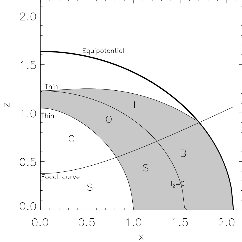
These properties are summarized in Fig. 2, where we have used the isochrone separable potential of the triaxial Abel model. The figure shows the -plane for a value of the energy that is large enough that all orbit families are populated. The thick outermost curve is the equipotential at this energy, the inner- and outermost decreasing curves inside the equipotential connect the points where the thin orbits cross the -plane perpendicularly, the intermediate decreasing curve corresponds to , and the rising curve is the focal hyperbola. The four areas corresponding to the different orbit families are also indicated (see §5.4 of vdV07 for further details).
This orbital structure depends crucially on the presence of a central core and is (partially) destroyed by the addition of a supermassive black hole and/or a central cusp (Gerhard & Binney 1985). Some orbits in these non-separable potentials do not conserve global integrals of motion other than the energy and may not all cross the -plane perpendicularly. The three types of tube orbits, including the thin tubes, are still supported cf. Schwarzschild (1993). Most box orbits are transformed into boxlets (Miralda-Escudé & Schwarzschild 1989) and orbits that occupy certain parts of phase space become chaotic. The amount of chaotic motion and the radial range inside which it is present depends on the central cusp slope (see §4.6).
4.3 Initial conditions
The orbits in our models are more complicated than those in a separable potential, as we use a more realistic MGE potential with a supermassive black hole. Still, we use the properties of separable models in our sampling of initial conditions. We sample the orbital energy implicitly through a logarithmic grid in radius. When the model has to reproduce observational data, it is important to sample the orbital energy on a grid with a minimum radius that is at least an order of magnitude smaller than the pixel size of the observations. In the case of Hubble Space Telescope data, this typically corresponds to arcsec. The outer grid radius is determined by our constraint that the grid must include per cent of the mass.
Each of the grid radii is linked to an energy by calculating the potential at . The orbital initial conditions are then sampled from a dense grid in the -plane. Since most orbits cross the -plane perpendiculary twice above it is not necessary to sample the whole plane. The double-countings are avoided by finding the location of the thin orbit curves iteratively: we launch orbits at different radii [keeping fixed] until the width of the orbit is minimal. This is similar to what was done in the axisymmetric three-integral models, where all orbits are short-axis tubes.
The starting points are selected from a linear open polar grid in between the thin orbit and the equipotential (the grey area in Fig. 2). The initial velocity in the direction is determined from and . This three-dimensional set of starting conditions is commonly referred to as the ‘ start space’ (Schwarzschild 1993). It is sufficient to launch orbits in only one direction when the density (or another quantity that is even in the velocity, such as the second moment) has to be reproduced. When the velocity (and odd higher-order velocity moments of the distribution function) is fitted in the model, the direction of the orbital motion is also important. This information could be taken into account directly by launching orbits in both the positive and negative -direction. However, the trajectories of the pro- and retrograde orbits are identical, which means it is much more efficient to include the counter-rotating orbits only at the fitting stage by reversing the velocity sign appropriately. This is only valid when figure rotation is ignored cf. Schwarzschild (1982).
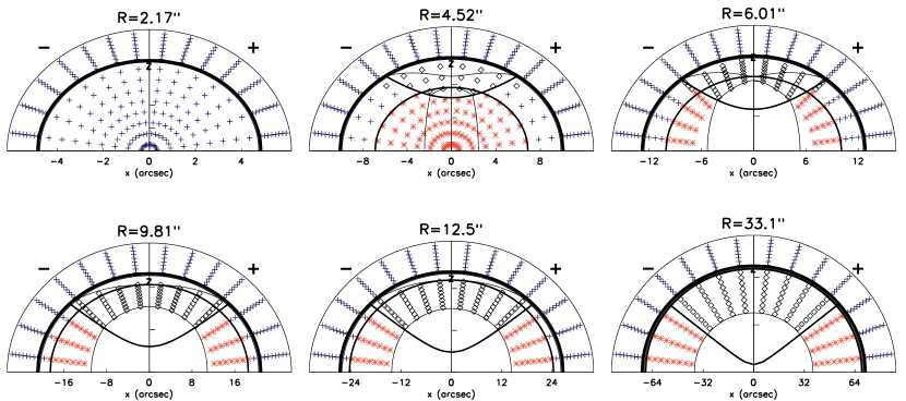
Since boxes are essential for the support of the triaxial shape (Schwarzschild 1979; Hunter & de Zeeuw 1992), a library with relatively few of them cannot be expected to reproduce a triaxial mass model. The () start space has few box orbits, especially at large radii (see Fig. 3). To make sure that the orbit library provides enough freedom in the outer parts of the model, we add additional box orbits, like Schwarzschild (1993). Box orbits always touch the equipotential (Schwarzschild 1979). We therefore sample start points on (successive) equipotential curves, using linear steps in the two spherical angles and . At each combination of () and , we use bisection to find the corresponding value of that is located on the equipotential. This three-dimensional set () of start conditions, the ‘stationary start space’ (Schwarzschild 1993), results in box orbits or boxlets only. Tube orbits always conserve the sign of at least one component of the angular momentum and therefore never reach zero velocity. Since the direction of the orbits in this start space is not important it is not necessary to add velocity mirrored copies of them during the fit.
By design the set of energies and angles in in both start spaces are identical, so that the orbits on the equipotential boundary of the start space have obvious neighbours in stationary start space. While not necessary, the size of the third dimension of the start spaces is chosen to be the same for consistency. Both sets of orbits can be represented in a single figure, by graphically connecting the corresponding starting spaces at the equipotential, as shown in Fig. 3, where selected energies of the triaxial Abel model (§ 4.1) are shown. In this figure we have overplotted the same lines from Fig. 2, which shows that our numerical scheme to locate the thin orbits indeed results in an orbit sampling from the correct region. The stationary start space intersects with the x-z start space at the equipotential. In the figure all the orbits in the stationary start space that are nearest to the equipotential are plotted just outside the equipotential. Subsequent rows in the stationary startspace are plotted radially outwards. A mirror image of the stationary start space is also plotted for symmetry.
4.4 Dithered orbit integration
The orbits in the start space are integrated numerically and their properties stored. The integration is done in Cartesian coordinates, using an explicit Runga-Kutta method of order 5(4) (DOPRI5 routine by Hairer, Norsett & Wanner 1993). With this method, the majority of the orbits can be integrated with energy accuracies of better than one part in . This routine is capable of dense output, which enables you to get a interpolated position and velocity at any time in current timestep during the integration.
To ensure numerical precision the Runga-Kutta integrator uses more steps where the orbital trajectory changes direction quickly. Since this usually happens when the ‘star’ is traveling with a high velocity, the integrated time steps do not represent the time-averaged path of the orbit. To make sure this is not a problem we use the dense output of the integrator, to sample the orbit on equal time intervals, ensuring that the orbits are properly time weighted.
Single orbits correspond to delta-functions in integral space, while the distribution function of a (partially) phase-mixed galaxy is expected to vary smoothly (Tremaine, Henon & Lynden-Bell 1986). This limitation may be reduced by combining nearby orbits (Richstone & Tremaine 1988; Rix et al. 1997). Here we extend this method by ‘dithering’ orbits in all three dimensions in the initial starting space. We do this by taking a bundle of orbits with different, but adjacent, initial conditions and sum their observables. This method is also used in the construction of axisymmetric models see Cappellari et al. (2006).
When calculating the starting spaces for the orbits we create more starting points for the dithering. We enlarge the sampling three-dimensional () start spaces five times in each direction. This leads to 125 orbits per bundle. The odd number five was chosen so that each bundle has a clearly defined central orbit (see figure 6 in Cappellari et al. 2006). The orbital properties of each of the orbits in each bundle are simpy co-added. As an alternative, it is be possible to apply some form of (Gaussian) weighting. In this way the orbit bundles could be made to overlap, but the effects of this have not been studied.
Effectively, the model thus contains 125 times more orbits. The dithering causes the orbital building blocks to be smoother, eliminating aliasing effects, especially when modeling spatially extended kinematic data. We found that this dithering is essential to obtain smooth orbital observables and remove numerical noise, using a limited amount of orbits.
4.5 Storage grids and symmetries
For spherical galaxies, it is in principle sufficient to store the orbital properties in one dimension, along a line. The three-dimensional model can be reconstructed afterwards by deprojecting the radial profile back onto the sphere. Similarly, axial symmetry allows one to carry out the calculations in the meridional plane only. Revolution of the model around the intrinsic short axis returns the three-dimensional intrinsic properties. As we restrict ourselves to stationary, non-rotating galaxies that are symmetric in the three principal planes, all orbital properties have to be calculated in only one octant. The properties in the other octants follow by symmetry.
The density of every orbit in the library is stored on a spherical grid in [ corresponds to the short axis and to the long axis]. The radial sampling is logarithmic with the inner and outer boundary set to zero and infinity. The angular grids and are sampled linearly between and . The grid has , and . This leads to 20 bins per radius and 300 bins in total, which is enough to ensure that the mass is reproduced well and the model is self-consistent. When fitting the model, the intrinsic mass grid is used as a constraint and is fitted everywhere with an accuracy of 2 % (see §5).
Similar to the intrinsic symmetries, the projected properties of spherical galaxies are one-dimensional and those of axisymmetric galaxies are symmetric in the projected axes. It is therefore sufficient to store the projected properties of spherical galaxies in one dimension and those of axisymmetric objects in one quadrant of the sky. The projected properties of triaxial galaxies are at most point-symmetric, with respect to the projected centre, which implies that the model-data comparison must be done in one half (or more) of the sky plane.
To convert the intrinsic coordinates (,,) to the projected coordinates (,,) we use eqs. (2) and (3). After this step the PSF is included by randomly perturbing the projected coordinates (,) with a probability described by the MGE PSF, before being included into the observational apertures (identical to Cappellari et al. 2006). We use a three-dimensional rectangular storage grid in the projected Cartesian coordinates and and the line-of-sight velocity in the the sky plane. The resolution and rotation of this grid is adapted to the kinematical data that have to be reproduced. Optionally, the observational apertures can be binned as a final step to match any obervational binning.
| Position | Box | L-tube | S-tube |
|---|---|---|---|
Only orbits with the correct degree of symmetry can be used to reproduce the density and potential. All orbits in a separable potential are indeed eightfold symmetric, but this need not be the case for resonant and irregular orbits in more general potentials. These orbits can therefore not be used directly in the reconstruction of the potential and density that we are interested in. This does not mean that they are useless, as we can enforce the required symmetries by apply a folding scheme to these orbits. Again, this scheme is similar to what is done for axisymmetric potentials, except that only orbits that are not symmetric with respect to the plane have to be corrected in that case [e.g. 1:1 () resonances, Richstone 1982].
The folding scheme is based on the fact that a given asymmetric orbit has up to seven mirror images that are obtained by reflection in the principal planes (see the first column of Table 2). These mirror images are also supported by the potential, but do not appear in the library because we sample orbital initial conditions only from one octant. All eight mirror orbits have identical properties and are equally useful for the model. We may therefore add these eight orbits to obtain an orbit that has three planes of symmetry. In practice, this is done as follows. During orbit integration, the orbital weight that corresponds to a given point is equally distributed over the eight mirror points. The contributions to both the intrinsic and projected density of all eight points are added up into one orbital building block. In this way, orbits that are asymmetric are included correctly, while orbits that already are eightfold symmetric are simply sampled more densely.
More attention is required when calculating the kinematical observables of the orbital building blocks. If we reflect the velocities in the same way as the coordinates, the total orbital building block has no net angular momentum. This is only correct for box orbits, while tube orbits, which are essential when fitting to the observed velocity field, conserve the sign of at least one component of the angular momentum vector. Therefore, the sign of the angular momentum of these orbits must be preserved also in the total orbital building block. This is ensured by classifying the orbits on the basis of their angular momentum properties. Box orbits oscillate in all three directions, so that no components of the angular momentum are conserved, while long-axis and short-axis tubes conserve the sign of the angular momentum parallel to the long and short axis, respectively. This allows us to distinguish orbits by checking for which angular momentum component(s), if any, the sign is conserved during orbit integration. In doing this, inner and outer long axis tubes cannot be recognized separately. This is, however, not a problem for the present application (cf. Schwarzschild 1979). As can be seen from Fig. 3, where we have plotted the different orbital types with different symbols, the numerical classification agrees with the analytical calculations.
We then apply the following scheme for reflections in the principal planes (see Table 2). Box orbits: the average angular momentum is zero, which allows us to reflect the velocity components in exactly the same manner as the coordinates. Long-axis tube orbits: the sign of the angular momentum around the long axis, , is conserved, which means that must be the same for all eight mirror points. Short-axis tube orbits: the sign of is conserved.
4.6 The influence of a central mass concentration
Central mass concentrations have considerable influence on the orbital structure of the galaxy as a whole and may induce chaotic behaviour. In an axisymmetric potential, the non-integrable regions of phase-space (usually referred to as the Arnold web) are not connected. This means that the diffusion of chaotic orbits is limited and their influence on the model is probably not significant, which justifies the fact that chaotic orbits are not treated in a special manner in axisymmetric models. Realistic triaxial potentials can support a much larger fraction of chaotic orbits. The overall amount of chaotic motion depends on the cusp slope and on the mass of the central mass concentration (Gerhard & Binney 1985; Merritt & Fridman 1996; Valluri & Merritt 1998), but the different orbit families experience fundamentally different effects, due to the central mass concentration
The box orbits that are started from the inner most equipotentials are very difficult to integrate numerically. The central accelerations are large and the time-steps that are required to conserve the integration accuracy are correspondingly small, resulting in prohibitively long orbital integration times. This effect can be reduced by using a nonzero value for the softening length that was introduced in §3.8. The DOPRI5 routine that we use to integrate the orbits varies the time steps to match the desired accuracy. We found that even orbits that pass close to the black hole can be integrated with an accuracy of in a reasonable time. The softening length that we used is typically two orders of magnitudes smaller than the radius of the sphere of influence of the black hole. This sphere of influence is defined as , which is the radius inside which the black hole potential dominates.
Test particles that are dropped from equipotentials at somewhat larger distances from the black hole are scattered off their original (box) orbits and may become chaotic (Gerhard & Binney 1985). The trajectories of such particles can be described by a series of regular segments and, given enough time, will fill most of the equipotential that corresponds to the orbital energy. Since equipotentials are rounder than equidensity curves and box orbits are the backbone of the triaxial shape, this process may destroy the triaxial shape from the inside out (e.g. Poon & Merritt 2002).
Chaotic orbits are not time-independent, since their orbital densities do not average out on physical time-scales. In principle, this means that a Schwarzschild model with an orbit library that includes irregular orbits is not stationary. However, evolutionary studies of models that include chaotic orbits (Schwarzschild 1993) and N-body simulations (Merritt & Fridman 1996; Holley-Bockelmann et al. 2002) display no dramatical shape-changes, even after very long times. This means that a model with chaotic orbits may be stationary for as long as a Hubble time and Schwarzschild solutions can be constructed also for models that contain chaotic orbits.
The use of dithered orbital components (§ 2.2) is critical to create nearly time-independent models. In fact orbits started from similar initial conditions can follow very different trajectories. Because of the dithering single ‘sticky’ chaotic orbits do not play a major role, since orbits are always bundled with nearby orbits.
The influence of a central mass concentration on tube orbits is radically different. Low-energy tubes, which orbit at large radii, never approach the central mass concentration close enough to be significantly disturbed. Tubes that are launched from the principal planes close to the radius of influence of the black hole turn into precessing ellipses. Depending on the shape of the volume that the ellipse eventually fills, they may be labeled as pyramid orbits (Poon & Merritt 2002) or lens orbits (Sridhar & Touma 1999; Sambhus & Sridhar 2000). The precession rate of the ellipse is determined by the ratio of the stellar mass that is enclosed by the orbit and the central black hole mass. The integration time that is required for convergence of the orbital properties is therefore inversely proportional to the orbital radius.
4.7 Number of orbits
To summarize, we use two start spaces with three dimensions and , which are connected at the equipotential boundary of every energy. The total number of orbits in the fit, excluding dithering, is three times the number of orbits in the one start space, as the start space is used twice and the stationary start space once. The number of orbits is denoted as . Because of the dithering each effective orbit consists of 125 orbits, significantly smoothing the orbital component. The total number of orbits necessary to make a model is dependent on several factors: the number and spatial distribution of the observed kinematics, the size of the galaxy model and the shape of the potential.
The effect of the number of orbits can be studied by determining the quality-of-fit of the model as a function of the number of orbits. With increasing orbit numbers the decreases. When enough orbits are present, the model does not improve any more and the does not decrease anymore. In our test cases we find that the model do not improve considerably when the orbit library consists of 2000 orbits or more. Self-consistent models with smaller orbit libraries have significantly larger , due to the fact that there are not enough orbits to reproduce the mass, especially at larger radii. We therefore decided to use an orbital sampling of 21 equipotential shells with starting points each, totaling 3528 orbits.
5 Superposition and regularisation
To make a model with the computed orbits we need to combine the orbits in such a way that they fit the observations, while reproducing the (intrinsic) mass distribution for self-consistency. Here we describe the construction of the orbital superposition and a way to ensure that our numerical solution is realistic.
5.1 Finding the orbital weights
The model has two components that need to be fitted: The kinematic observations and the (intrinsic and projected) mass distribution. The kinematics are fitted using linearly superposed mass-weighted Gauss-Hermite (GH) moments (Rix et al. 1997). The fit is done by combining the orbits linearly by assigning each orbit an orbital weight (). These orbital weigths directly represent the mass in each orbit and must therefore be positve (0).
The intrinsic mass grid (§4.5) and the aperture masses (the total amount of mass in each observed aperture: the zeroth GH moment) must be added to the fit to ensure that the model is self-consistent with the density in which the orbits were calculated. Often this is done by including them in the fit as an ‘observable’ (e.g., van der Marel et al. 1998; Valluri et al. 2004). However they are not actually observed and therefore it is difficult to assign an error. To include them into the fit they are usually assigned a hand-tuned fractional error so that the mass is reproduced well without influencing the fit of the kinematics. Here we use a different approach by including them as ‘constraints’ with bounds in the fit (similar to Richstone & Tremaine 1988). This means that the orbital superposition reproduces the intrinsic and aperture masses to within 2 % at all times, while finding the best-fitting kinematics. The total normalised mass of all the orbital weights is fixed using an equality constraint.
The reason for including constraints is that the mass can almost always be reproduced up to numerical percision (van der Marel et al. 1998; Poon & Merritt 2002) and is thus not relevant for finding the best-fit solution. We only want the mass to be reproduced to within 2 %, because this is the typical accuracy of (the MGE of) the observed surface brightness. Within these bounds the solver allows the mass to vary to find the best-fitting kinematics in the least squares sense.
We use the sparse quadratic progamming solver QPB from the GALAHAD library (Gould, Orban & Toint 2003) to make the superposition, as this algorithm is capable of fitting the kinematics in the least squares sense while satisfying mass constraints. This algorithm optimizes the orbital weight in the least squares sense:
| (24) |
subject to the positivity constraint
| (25) |
and the linear constraints,
| (26) |
Here is the projection matrix whose columns give the model contribution of every orbit to the kinematical observables . The matrix is a projection matrix giving the model contribution of the orbits to the mass in the various apertures and is the mass derived by integrating the MGE model over the projected apertures and intrinsic mass grid. The total number of constraints in the fit () is 300 (intrinsic mass grid) + 1 (total mass) + the number of apertures (aperture masses).
The quality of the model is determined by measuring the discrepancy between the model and the observations for different values of the input parameters. This is done by calculating the , defined as
| (27) |
in which is the number of observables (the number of apertures times the GH moments), is the observation for the th observable, is the model prediction and is the uncertainty that is associated with this value (the observational error).
5.2 Regularisation scheme
The quadratic programming problem to be solved is ill-conditioned in most applications, due to (close to) degenerate orbits. As a consequence, the orbital weight distribution for the solution with the smallest may be a rapidly varying function, which is not likely to be realistic (Merritt 1993; Verolme & de Zeeuw 2002). This effect can be reduced by adding linear regularisation equations to the problem (e.g., Zhao 1996; Rix et al. 1997), which is also known as ‘damping’ in the field of linear programming. Such regularisation terms can be added to force the orbital weights towards a smoother function by minimizing their higher-order derivatives.
Our two start spaces are sampled in three dimensions and and they are connected at the equipotential boundary. The three dimensions of the start space roughly correspond to the three integrals of motion (in a separable potential). We can thus enforce smoothness of our solution by adding regularisation terms to our minimisation routine in each of the three directions of our start space. We adopt the second order finite differencing (Press et al. 1992) regularisation from Cretton et al. (1999), so for each orbit we add three equations to the array A given above, and minimises them in a least squares sense
| (28) |
where represents the orbital weight at position in the start space grid. The weights are added to include the radial energy dependence of the model. It is estimated, a priori, as the normalised mass enclosed by each radial shell in the start space
| (29) |
where is the number of orbits. The regularisation error determines how much smoothing is perfomed. Increasing increases the amount of smoothing. The optimal value of this is usually time-consuming to determine (see, e.g., Cretton et al. 1999). However, it has been shown elsewhere that a theoretical axisymmetric galaxy with a two-integral distribution function can be accurately reproduced by using this approach (Verolme et al. 2002; Cretton & Emsellem 2004). Applications of the axisymmetric Schwarzschild method have often used a value of as regularisation (Cappellari et al. 2002; Krajnović et al. 2005). As we will show in the next section it is also acceptable for the triaxial method.
5.3 Testing the regularisation
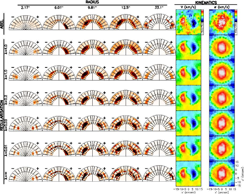
In the companion paper the DF of the triaxial test model is compared directly in terms of the integrals of motion (§ 5.4.3 in vdV07) and we find that the recovery of the DF is consistent with the quality of the input kinematics (Figs 12 and 13 in vdV07). The triaxial test model is ideally suited to test regularisation. To do this we compare the orbital mass weights directly. The top row in Fig. 4 displays the computed orbital weights and kinematics for the triaxial Abel model from vdV07. The other rows show the orbital weights and kinematics for the best-fit Schwarzschild model with decreasing regularisation from top to bottom. The orbits at the radius of and are outside the range where they are constrained by the kinematics, and as such the orbital weights for the Schwarzschild models are not expected to compare well with those of the Abel model.
The distribution of (analytical) orbital weights for the Abel model is smooth with some sharp peaks. The reconstructed orbital weights from the Schwarzschild agree well with the analytical orbital weights, except for high values of , which corresponds to strong regularisation. The orbital weights of strongly regularised models are distributed more smoothly, adjacent orbits receive similar weight and the kinematics start to change. From Fig. 4, we see that the kinematics is affected by the regularisation at , and thus the optimal regularisation in this case has to be chosen to be . This will give satisfactory orbital weights, and kinematics that are consistent with the observations. The comparison is best for a
There are many reasons why the reconstructed orbital weights do not exactly match the analytical orbital weights. Most of them are minor numerical and discretisation effects. For example: (i) The Schwarzschild method samples the galaxy with discrete orbits (computed in the reconstructed potential), which are related to the DF via their phase-space volume (Vandervoort 1984). The resulting orbital mass weights are evaluated in an approximated and numerical way (§5.4 in vdV07). (ii) Some symmetric orbits appear twice (or more often) in the orbit library. Without regularisation the (quadratic) solver ignores the second identical copy of this orbit, as they do not improve the fit. However these orbits do get assigned weight in the test case. A good example of this are the box orbits in the start space, as they are added twice to the fit [like all orbits]. These differences are only visible in this direct comparison of the orbital weights.
To estimate the effect of regularisation on the kinematical fit more quantitatively, we investigated the difference between the models with different values of the regularisation . For the best-fit model with 2370 kinematical observables the total is 2588. Adding regularisation does increase the of the model. With (little regularisation) it does not affect the fit to the kinematics (). When increasing furter to 0.2 or even 4 (very strong regularisation), the changes to and , respectively. These numbers reflect what one sees in Fig. 4: for the kinematical fit does not change visibly, whereas for higher (stronger regularisation) the kinematical fit becomes rapidly worse.
One other important question is whether the regularisation changes the recovered input parameters, including the viewing angles, mass-to-light raio, anisotropy and black hole mass. This is nearly impossible to test with real galaxies, as their properties are unknown. The Abel model has known parameters and was used to test the recovery. We found that there is no difference in the best-fit parameters when a regularisation of was chosen. The confidence intervals of the parameters do become smaller by using regularisation. This is expected, as the added regularisation terms decrease the freedom of the model and therefore increase the .
A notable exception, that we do not test here, is the recovery of the black hole mass. There are often few observables in the models near the sphere of influence. The number of mass bins near the black hole is extremely limited and the kinematical observations inside the sphere of influence of the black hole is very limited, usually less than 10 observables. In this scenario it is conceivable that regularisation is needed, as the model might otherwise adapt the orbital structure to be able to accomodate the black hole (see also e.g., Magorrian 2006). Recovery of the black hole mass using regularisation will be presented elsewhere.
6 Tests on the triaxial Abel model
We test our method on the triaxial Abel model from the companion paper vdV07, introduced in §4.1 and already used in § 5.3 above. Here, we outline further tests done on the Abel model.
6.1 Internal orbital structure and DF recovery
In vdV07 the best-fit triaxial Schwarzschild model to the input triaxial Abel is presented. The Schwarzschild method only uses the information that can be observed in real galaxies, i.e. the two-dimensional surface brightness and the two dimensional stellar kinematics. The resulting best-fit model is an excellent fit and has a (reduced) per degree-of-freedom of .
Since Schwarzschild models only fit the projected observables it is not obvious that these models can recover the three-integral DF and the internal structure of the test model. By comparing the mass weights of the Schwarzschild model to the DF of the test model, vdV07 demonstrate that both the internal orbital structure and DF are recovered, with an accuracy similar to the typical (simulated) errors on the kinematics.
6.2 Recovering the global parameters
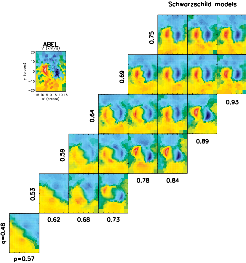
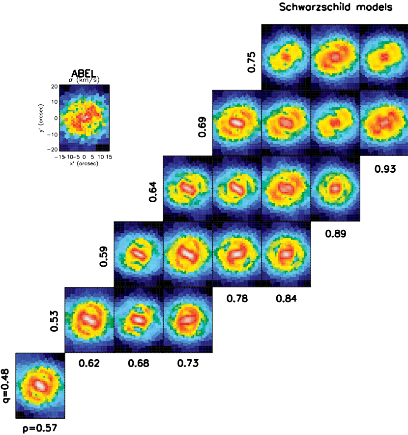
When constructing Schwarzschild models of the Abel model, we expect the kinematics of the Schwarzschild model to vary when changing intrinsic shape parameters , and thus the viewing angles . The most obvious are the change of the zero-velocity curve as the projected axes change on the sky. Also, the characteristics of the orbits in the model are dependent on the shape of the potential. These effects are shown in Fig. 5, by showing models of the analytic test data in linear steps of 0.05 in or . The models become significantly worse when changing the parameters away from the correct values. This shows that different intrinsic shapes support different orbits and that one cannot expect a model with the wrong potential to be able to fit the kinematics in all cases.
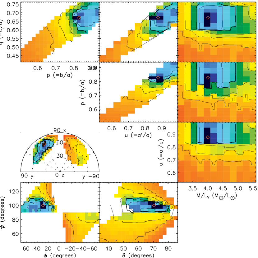
To search the global parameters we sample the parameter space, by making linear steps of 0.1 M⊙/L⊙ in , and 0.05 in , and (resulting in 100 different intrinsic shapes). For each corresponding Schwarzschild model, the changes are quantified by the goodness-of-fit parameter . To visualize this four-dimensional parameter space, we calculate for a pair of parameters, say and , the minimum as a function of the remaining parameters, and in this case. The contour plots of the resulting marginalized for all different parameters for the Schwarzschild models fitted to the observables of the Abel model are shown in Fig. 6. Since we sampled in intrinsic shape and not in viewing direction, the viewing angle sampling is not uniform. In particular the very round models, which are independent of are not represented properly. To this end, we create a dense grid in and interpolate the linearly over this dense grid, resulting in the contour plots of in Fig. 6.
The input parameters for which the simulated observables of the Abel model were obtained are M⊙/L⊙ and . As outlined in § 3.7, the latter viewing angles convert to the intrinsic shape parameters , given the average projected flattening of (the MGE model of) the surface brightness. These input parameters are denoted by a red diamond in the contour plots of Fig. 6. We find that the input and (and hence also the viewing angles) of the Abel model are accurately recovered, with a typical uncertainty of 10 % or less.
Krajnović et al. (2005) suggested that the recovery of the inclination for axisymmetric models is degenerate, which seems in conflict with our recovery of the intrinsic shape. However, the kinematics of the Abel model have a significant feature, namely a orthogonal decoupled core, and this makes it plausible that the viewing angles are constrained quite strongly. We verified that for galaxies with no such distinguished kinematic feature, e.g., in the case of a (nearly) zero mean velocity map like for M87, the intrinsic shape is not well constrained.
7 Application to NGC 4365
We now apply our method to NGC 4365, one of the prototypical galaxies with a kinematically decoupled core (KDC). It is a giant E3 elliptical and it was one of the first objects in which minor axis rotation was discovered (Wagner, Bender & Moellenhoff 1988; Bender, Saglia, & Gerhard 1994). The peculiar velocity structure of this galaxy was partially unraveled by multiple long-slit observations (Surma & Bender 1995), but the full two-dimensional kinematical structure was only revealed with the integral-field spectrograph SAURON (Davies et al. 2001).
Kinematically decoupled cores can be the result of a merger event, but can also occur when the galaxy is triaxial and supports different orbital types in the core and main body (Statler 1991). Davies et al. (2001) studied the first option and investigated the link between the kinematics and the line-strength distribution of NGC 4365. They found that the core and the main body are of similar age and that any mergers that led to the formation of the KDC must have occurred at least 12 Gyr ago, as otherwise younger stellar populations would have been detected. The orbital structure that supports the KDC and the main body cannot be observed directly and must be inferred from dynamical models. Statler et al. (2004) studied the viewing angles and triaxiality of the system using an approach developed by Statler (1994a), which uses bayesian analysis to fit analytic solutions of the continuity equation to an observed velocity field. They found NGC 4365 to be strongly triaxial and seen almost along the long axis. The triaxial Schwarzschild method that was presented in the previous sections allows us to build comprehensive dynamical models of this galaxy and investigate its intrinsic structure.
7.1 Observations
NGC 4365 was observed with SAURON on the nights of March 29 and 30, 2000, for two different pointings, with an overlap in the central region. The exposures were combined and rebinned into a map with a slightly better spatial sampling (0.8 arcsec, compared to 0.94 arcsec for the individual lenslets) and a coverage of 33 63 arcsec. Davies et al. (2001) give a full description of the observations.
To increase the signal-to-noise () ratio to sufficient levels for accurate determination of the kinematics, the datacube was spatially binned into 964 non-overlapping bins using the two-dimensional Voronoi binning of Cappellari & Copin (2003). A minimum of 100 per spectral element was imposed. However, many of the spectra have a much higher value (up to ), and more than one quarter of the spectral elements remain unbinned. The stellar kinematics where extracted using the penalised pixel-fitting method (pPXF) of Cappellari & Emsellem (2004). For every Voronoi bin we extracted the velocity , velocity dispersion and the higher-order GH moments and of the stellar LOSVD.
The SAURON spectra have very high so that the LOSVD can be reliably extracted from the data, however care has to be taken to minimize the effect of template mismatch, which dominates the error budget in the bright, high- central regions of the galaxy. To this end an accurate template was determined during the pPXF fit using the stars of the MILES library (Sánchez-Blázquez et al. 2006), which span a large range of stellar atmospheric parameters. Out of the MILES stars, only 14 are selected by pPXF to provide an accurate match to the observed average galaxy spectrum, with an rms scatter in the residuals of only 0.17 %. From the observed residuals and Fig. B3 of Emsellem et al. (2004), we infer an upper limit of on the systematic error of the GH moments, due to any remaining template mismatch.
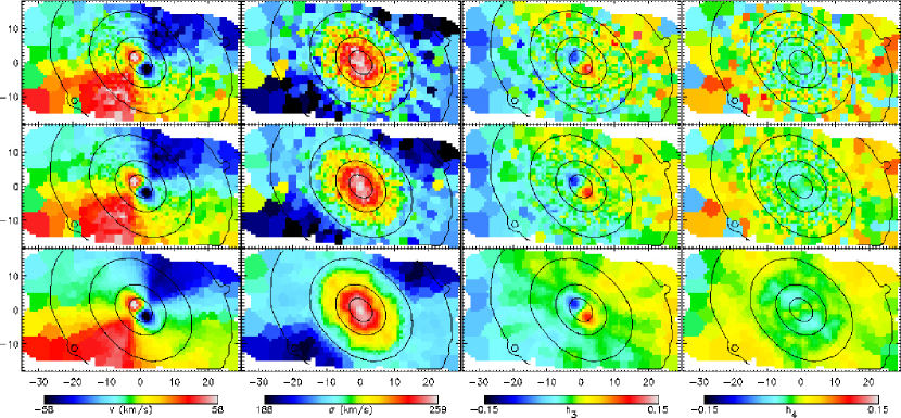
The re-reduced kinematics, shown in Fig. 7, are a significant improvement over the kinematics shown in Davies et al. (2001). They show a core in the inner arcsec that rotates around the minor axis. At larger radii the stars rotate around an axis offset by 82∘, which is evidence that the system is intrinsically triaxial. The peak mean streaming velocities are 55 km s-1. The dispersion peaks at a value of km s-1.
7.2 Mass model
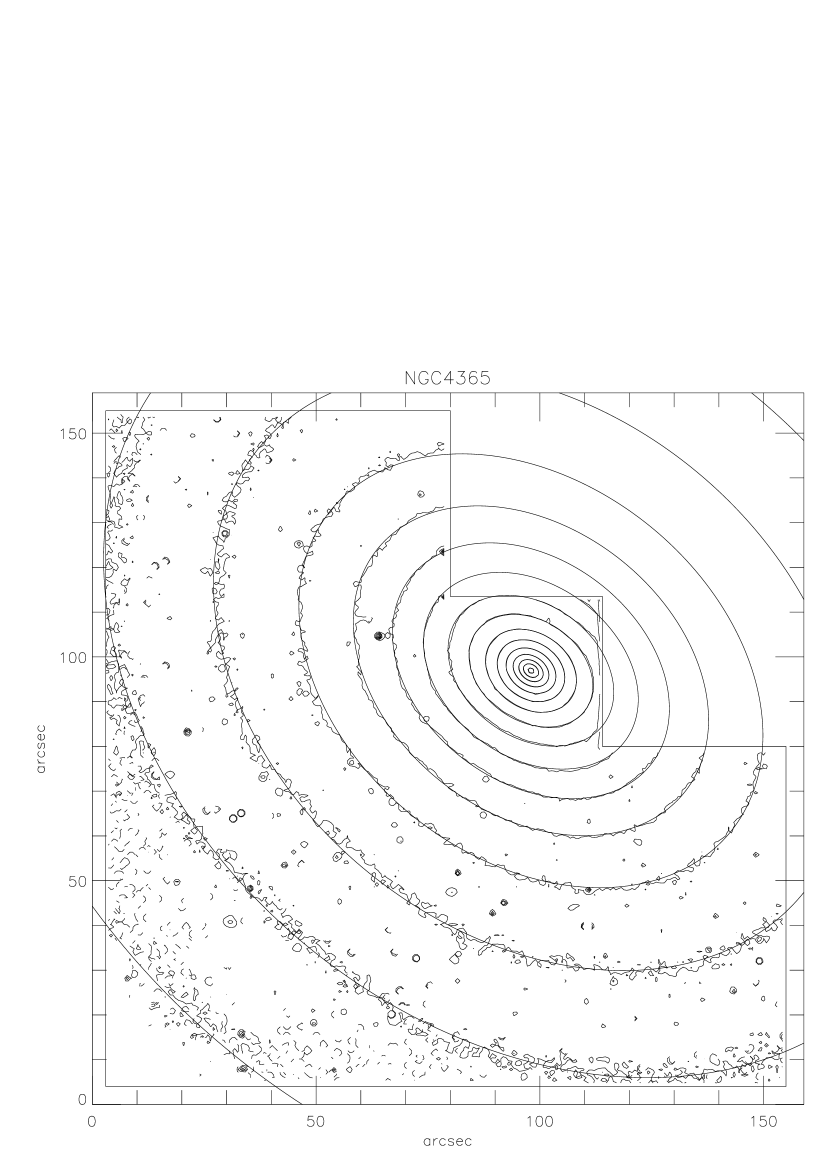

We used an HST/WFPC2/F814W image and a ground based image of NGC 4365 obtained with the 1.3m McGraw-Hill at the MDM observatory (from Falcón-Barroso et al., in prep.) to make an MGE (mass) model, using the software by Cappellari (2002). We ensure that the model is the roundest that is consistent with the observations. This is done by setting a lower limit to the allowed projected flattening of 0.67 and an upper limit of 4.5∘ on the difference in position angle between the individual Gaussians. The modest difference between the RMS-error of the free model (0.99 per cent) and the constrained MGE-model (1.02 per cent) suggests that these constraints do not lead to systematic errors in the mass model. The parameters of the MGE-model are given in Table 3, the surface brightness map and the MGE model fit are shown in Fig. 8.
| j | (L⊙,I pc-2) | (arcsec) | (∘) | |
|---|---|---|---|---|
| 1 | 3.424 | -1.024 | 0.800 | 0.0 |
| 2 | 3.319 | -0.727 | 0.800 | 0.0 |
| 3 | 3.238 | -0.320 | 0.800 | 0.0 |
| 4 | 3.435 | -0.027 | 0.670 | 0.0 |
| 5 | 3.820 | 0.138 | 0.709 | 0.5 |
| 6 | 3.740 | 0.402 | 0.698 | 0.8 |
| 7 | 3.576 | 0.648 | 0.798 | 0.0 |
| 8 | 3.106 | 0.955 | 0.737 | 0.0 |
| 9 | 2.874 | 1.224 | 0.739 | 0.0 |
| 10 | 2.400 | 1.499 | 0.741 | 3.5 |
| 11 | 2.122 | 1.833 | 0.775 | 3.6 |
| 12 | 1.329 | 2.362 | 0.670 | 4.5 |
7.3 Dynamical models
We calculate triaxial Schwarzschild models using orbit libraries of orbits, 2352 of which are started in the -plane, the remaining are dropped from the equipotential. We assume a distance of 23 Mpc for NGC 4365 (Mei et al. 2005). The assumed distance does not influence our conclusions about the internal structure of the galaxy, but lengths and masses scale linearly with the distance, while mass-to-light ratios are inversely proportional to the distance.
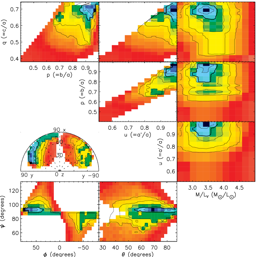
A given triaxial model is determined by the mass-to-light ratio , the shape parameters — or equivalently, the viewing angles — and the mass of the central black hole. We fix the latter to M⊙, consistent with the black hole-sigma relation (Tremaine et al. 2002), as the SAURON observations do not have enough spatial resolution to resolve the radius of influence of the black hole and therefore can not constrain the mass directly. Given a typical flattening of of the Gaussians in the MGE model (Table 3), we sample linearly in steps of 0.06. This results in 96 different intrinsic shapes which we combine with values sampled linearly in 11 steps, from 3.0 to 5.0 in solar units. This results in a total of 1056 Schwarzschild models, for each of which we compute the goodness-of-fit to the observations via . The resulting models show a smooth gradient in as can be seen in the contours in Fig. 10. As before (see § 6.2), to avoid an incomplete sampling in viewing angle space, we oversample in before computing the correspinding contours in .
7.4 Best-fit model
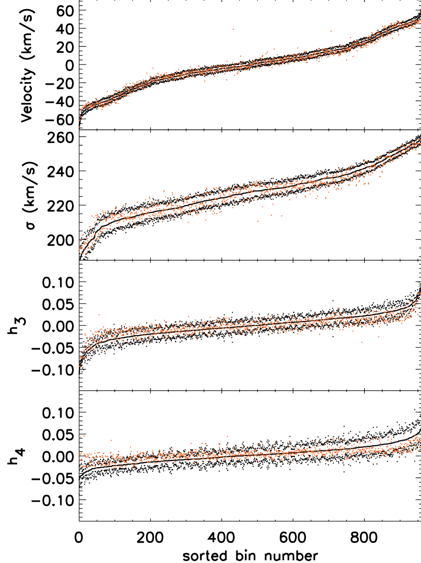
The best-fit model (the model with the lowest ) is shown in Fig. 7. To be able to estimate the quality of the fit, Fig. 9 shows the residuals per velocity moment. Each panel shows a moment sorted in order of increasing value. The observed moment is indicated by the black line, with errors shown as black dots. The red dots represent the corresponding values from the best-fit model, which is in good agreement with the data. The corresponding , which implies a per degree-of-freedom (DOF) of 1.1. Statistically the standard deviation of the is . Given that we have 3856 observables in our model and less than 10 parameters (), the expected scatter in the is much larger than the customary criterion. We therefore treat as a one sigma (68%) result. The best-fit parameters are then M⊙/L⊙ (in -band) and the intrinsic shape parameters .
The best-fit is just consistent with the value of M⊙/L⊙ predicted by the - relation derived from axisymmetric models by Cappellari et al. (2006), using a km s-1 for this galaxy222The velocity dispersion is derived from the SAURON kinematics by luminosity-weighting all the spectra within one effective (half-light) radius and fitting a single Gaussian LOSVD.. It is interesting to see that the best-fitting does not vary significantly with any of the other model parameters as can be seen in the contour plots in Figs. 10. For example, even for models with a non-optimal value of or , still the best-fit M⊙/L⊙. The total mass of the model, obtained by converting the total luminosity to mass using the best-fit value is M⊙.
7.5 Intrinsic shape
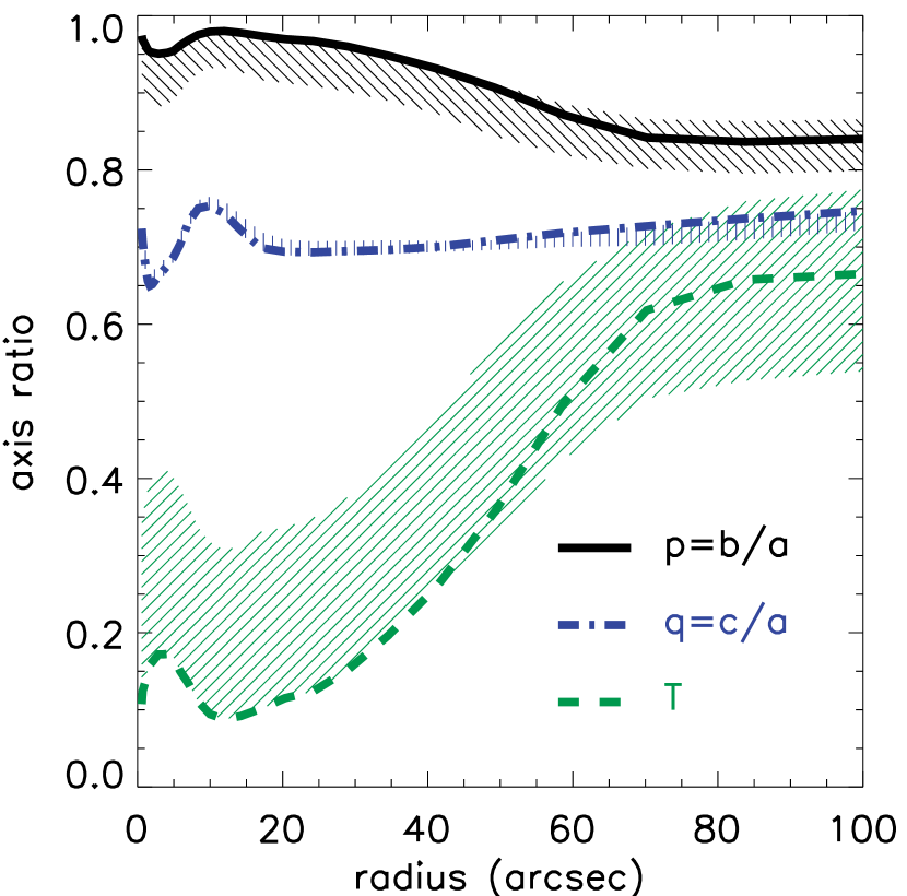
In Fig. 11, we show the intrinsic shape parameters as a function of radius of our best-fit model. Inside the central 35′′, where we have the kinematic observations, the shape of NGC 4365 is fairly oblate, with , and the triaxiality parameter . Further out – outside of the area where observed kinematics are available – the reconstructed density becomes more prolate. This is caused by the drop in to , while stays approximately the same. As a result the triaxiality rises with increasing radius to .
The axis ratios found by Statler et al. (2004) using velocity field fitting of the SAURON data are , which are just outside our 99 % confidence, and do not agree with their claim of strong triaxiality () inside 35′′ of the galaxy. Their lower limit on the triaxiality is not consistent with our measurement in the center. We return to this below.
The corresponding best-fit viewing angles are . To give an indication of the uncertainty of these values we show a Lambert azimuthal equal area projection of and in Fig. 10. This is comparable to a similar projection in Statler et al. (2004, their Fig. 4). Our best-fit viewing angle is also not consistent with theirs. The velocity field fitting (VF) method does not include the dispersion and other higher-order velocity moments and assumes a plausible solution of the continuity equation, while our Schwarzschild method does fit higher moments up to al least and does not enforce any constraints on the DF.
The effect of the higher moments on the inferred shape can be studied by making models without them. We find that excluding has no significant effect on the recovered shape. Removing and/or lower moments and (representing the dispersion and mean velocity) changes the best-fit shape significantly and the reconstructed LOSVD of these models show significant deviations from Gaussian. These models are therefore not a good representation of the observed LOSVD. This tests show that the Schwarzschild models need at least to accurately recover the inferred shape and observed LOSVD.
To compare our modeling to the VF method directly, we made models where we only fit the mean velocity. We find that these models are completely degenerate and no minimum could be found. Instead of our least squares approach a likelihood method could be used to find a solution in the probabilistic sense, however such methods are unpractical for Schwarzschild models, because of the many iterations required. The VF method does use Bayesian analysis, with a prior on the dispersion.
For NGC 4365 to be a pure long-axis rotator with a KDC that consists purely of short-axis tubes, we expect a best-fitting misalignment angle that coincides with the observed kinematic misalignment of (or the symmetric 98∘). In fact, all the models with ∘are strongly ruled out and we conclude that NGC 4365 is not consistent with a pure long-axis rotator.
7.6 The orbital structure
The observed kinematics that go out to ′′ show that NGC 4365 must be intrinsically triaxial, due to the kinematically decoupled core and the misaligned large scale rotation. This seems to be in conflict with the (nearly) oblate axisymmetric shape inside 30′′of our best-fit model (Fig. 11), as this shape does not support the rotation around the major axis seen in the observed kinematics.
Fig. 12 shows the cumulative mass per orbit-type as a function of intrinsic radius. As expected from the shape in the inner region the stars on short axis tube orbits are dominant, accounting for 75% of the mass inside . The stars on long axis tubes become significant in the model only outside .
To understand the rotation seen in the observations we look at the balance of stars on prograde and retrograde orbits, shown in Fig. 12. It shows that the stars in the KDC are on prograde short axis orbits inside , while up to the stars on short axis orbits do not have a preferred rotation direction. Only 15% procent of the stars inside move on long axis orbits, but nearly all of them move in the retrograde direction, and thus contribute to the observed mean velocity.
To make the link between the orbital structure and the observations, we show the unbinned kinematics of the stars on each type of orbit individually, extrapolated over a region larger than the orginal observations in Fig. 13. The mass fraction, velocity and dispersion field are shown for () all stars, () stars on prograde short axis orbits, () stars on retrograde short axis orbits, () stars on prograde and retrograde short axis orbits combined, and () stars on long axis and box orbits combined.
In the decomposition of Fig. 13 the stars on prograde and retrogrode short axis orbits have large velocities ( km s-1, km s-1) in opposite directions and the combination of them lead to a velocity field with very little rotation ( km s-1) and a high dispersion field ( km s-1). The stars on long axis orbits also rotate quickly ( km s-1) and although they contribute only % of the mass, the large velocity adds significantly to the large scale rotation seen in the observations.
Two other galaxies NGC 4550 and NGC 4473 show very similar features to NGC 4365, both have unusually high sigma along the major axis (Emsellem et al. 2004). They both consist of two counterrotating disks, similar to the two main components in NGC 4365: the prograde and retrograde short axis orbits (Rix et al. 1992; Cappellari et al. 2007).
The KDC is not very distinct in the decomposition (Fig. 13) and is perhaps only an appearance. The only way to really disentangle the KDC is through the unbalance of the central stars on prograde short axis orbits (Fig. 12). However, in the orbital weights (Fig. 14) the KDC seems an integral part of all the stars on prograde short axis tube orbits as these stars are continuously distributed in orbital weights. It is therefore difficult to see the KDC as a distinct kinematic component.
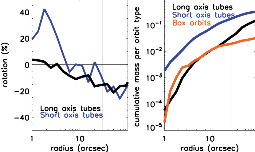
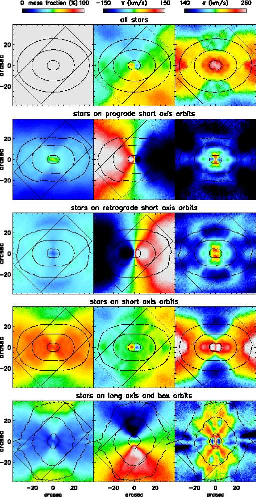
8 Discussion and Conclusion
We have presented a flexible method to build dynamical models of triaxial early-type galaxies, allowing for position angle twist and ellipticity variation in their surface brightness, as well as a central supermassive black hole. The method is based on Schwarzschild’s orbit superposition technique and uses the observed surface brightness distribution and observed kinematics to make a triaxial model of the observed galaxy. Our models can be constrained by observations of the full line-of-sight velocity distribution.
We discussed tests of our method on the triaxial Abel model with a separable potential from vdV07, which illustrates the accuracy of our orbit classification method and the effect of regularisation. Tests with the viewing angles showed that we can constrain the intrinsic shape of galaxies with significant structure in their velocity field.
We also presented results of an application on two-dimensional data of the E3 galaxy NGC 4365, obtained with the integral-field spectrograph SAURON. We showed that our method is capable of reproducing the main observational features to within the errors. We found a best-fitting (-band) stellar mass-to-light ratio of in solar units and best-fitting viewing angles of ()= (). The characteristic axis ratios are , inside . By applying a simple regularisation scheme, we were able to determine the distribution of orbital weights, which provided us with a view on the orbit structure of this galaxy. We find the inner part to be nearly oblate axisymmetric, with most of the stars equally divided on prograde and retrograde short axis tube orbits. Further out the galaxy becomes more triaxial, and the stars orbit on both long axis and short axis tubes. The KDC seen in the observations is not dynamically distinct from the main body of the galaxy. More evidence for the idea that the ‘decoupled core’ is part of the main body of the galaxy, comes from the stellar ages determined by Davies et al. (2001). The ages of the stars where determined to be at least 12 Gyr and they do not show a strong dependence which radius. Overall our orbital structure is consistent with the results from Statler (1991) and Arnold et al. (1994).
An important consideration is the stability of triaxial galaxies. A significant fraction of the centrophilic box orbits can become chaotic in the presence of a central cusp or a supermassive black hole (Gerhard & Binney 1985; Valluri & Merritt 1998). As box orbits are crucial for supporting the triaxial shape, it is not evident whether a triaxial object with a central black hole can retain its shape over a Hubble time (Lake & Norman 1983). Earlier -body simulations of triaxial galaxies in which a central mass concentration is grown indeed show a fairly rapid evolution towards a rounder shape in the inner parts (e.g. Merritt & Quinlan 1998; Valluri & Merritt 1998), but these results were challenged recently (Holley-Bockelmann et al. 2002; Poon & Merritt 2002). The intrinsic shape of our best-fit model is nearly oblate axisymmetric in the centre, and more triaxial further out. This might be a sign of evolution towards a axisymmetric shape, induced by the central massive black hole from the inside out. Clearly, we need to obtain a better understanding of whether triaxial galaxies can reach stationary equilibrium and if not, what the time-scale of the transition toward a nearly spheroidal shape is.
The extension from an axisymmetric to a triaxial implementation of Schwarzschild’s method opens up a wide range of applications. For example, while the mass of the central black hole seems to be correlated with other properties of the galaxy (Ferrarese & Merritt 2000; Gebhardt et al. 2000; Tremaine et al. 2002), nearly all black hole estimates were derived with dynamical models of (edge-on) axisymmetric models. In such models, the increase in line-of-sight motion towards the center that is seen in high-resolution observations of many nearby galaxies can indeed only be explained by a black hole. In triaxial systems, box orbits provide an alternative way of creating motion along the line-of-sight (depending on the viewing angles, see e.g., Gerhard 1988). As a result, a given observed velocity profile may require a different black hole mass when the galaxy is allowed to be triaxial, which in turn may influence the black hole mass correlations if the intrinsic shape correlates with luminosity, as has been suggested.
Another area of interest is the validation of predictions on the halo shapes from galaxy merger (e.g., Wechsler et al. 2002) and CDM cosmology simulations (e.g., Navarro & Steinmetz 2000). They predict the existence of strongly triaxial halos as a result of merging. To confirm these simulations, our method can be used to measure the halo shapes of a representative sample of galaxies, using kinematical observation at large radii, where the halo mass dominates.
Our method can be further extended in a number of aspects. For example, we assumed that the galaxy as a whole is non-rotating. The reason for this is that inclusion of figure rotation further complicates matters (Schwarzschild 1982; Heisler, Merritt & Schwarzschild 1982), while it may not be crucial for the modeling of existing observations of giant elliptical galaxies. The fitting of kinematics can be improved by fitting the LOSVD directly or by using eigen-velocity profiles (Houghton et al. 2006). Additionally, the method can be enhanced to include line strength information and multiple stellar populations, to study the distribution of stellar ages and metallicities within galaxies. Even without additional extensions, the triaxial Schwarzschild method allows us to investigate the intrinsic structure and orbital make-up of early-type galaxies.
Acknowledgements
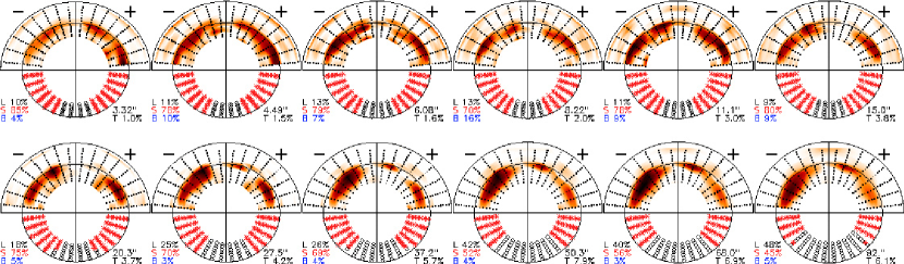
It is a pleasure to thank Eric Emsellem, Karl Gebhardt and Roeland van der Marel for a critical reading of an earlier version of the manuscript. We also like to thank Jesús Falcón-Barroso for the image of NGC 4365.
The SAURON project is made possible through grants 614.13.003, 781.74.203, 614.000.301 and 614.031.015 from NWO and financial contributions from the Institut National des Sciences de l’Univers, the Université Claude Bernard Lyon I, the Universities of Durham, Leiden, and Oxford, the British Council, PPARC grant ‘Extragalactic Astronomy & Cosmology at Durham 1998–2002’, and the Netherlands Research School for Astronomy NOVA. GvdV acknowledges support provided by NASA through grant NNG04GL47G and through Hubble Fellowship grant HST-HF-01202.01-A awarded by the Space Telescope Science Institute, which is operated by the Association of Universities for Research in Astronomy, Inc., for NASA, under contract NAS 5-26555. MC acknowledges support from a VENI grant 639.041.203 awarded by the Netherlands Organization for Scientific Research (NWO). Part of this work is based on data obtained from the ESO/ST-ECF Science Archive Facility.
References
- Aarseth & Binney (1978) Aarseth S. J., Binney J., 1978, MNRAS, 185, 227
- Arnold, de Zeeuw, & Hunter (1994) Arnold R., de Zeeuw P. T., Hunter C., 1994, MNRAS, 271, 924
- Bacon, Copin, Monnet, Miller, Allington-Smith, Bureau, Carollo, Davies, Emsellem, Kuntschner, Peletier, Verolme, & de Zeeuw (2001) Bacon R., Copin Y., Monnet G., Miller B. W., Allington-Smith J. R., Bureau M., Carollo C. M., Davies R. L., et al., 2001, MNRAS, 326, 23
- Bender (1988) Bender R., 1988, A&A, 202, L5
- Bender (1990) —, 1990, A&A, 229, 441
- Bender, Saglia, & Gerhard (1994) Bender R., Saglia R. P., Gerhard O. E., 1994, MNRAS, 269, 785
- Bertola, Bettoni, Danziger, Sadler, Sparke, & de Zeeuw (1991) Bertola F., Bettoni D., Danziger J., Sadler E., Sparke L., de Zeeuw T., 1991, ApJ, 373, 369
- Bertola & Capaccioli (1975) Bertola F., Capaccioli M., 1975, ApJ, 200, 439
- Binney (1976) Binney J., 1976, MNRAS, 177, 19
- Binney (1978) —, 1978, MNRAS, 183, 501
- Binney (1985) —, 1985, MNRAS, 212, 767
- Binney & de Vaucouleurs (1981) Binney J., de Vaucouleurs G., 1981, MNRAS, 194, 679
- Binney & Tremaine (1987) Binney J., Tremaine S., 1987, Galactic dynamics. Princeton, NJ, Princeton University Press, 1987, 747 p.
- Bissantz & Gerhard (2002) Bissantz N., Gerhard O., 2002, MNRAS, 330, 591
- Cappellari (2002) Cappellari M., 2002, MNRAS, 333, 400
- Cappellari, Bacon, Bureau, Damen, Davies, de Zeeuw, Emsellem, Falcón-Barroso, Krajnović, Kuntschner, McDermid, Peletier, Sarzi, van den Bosch, & van de Ven (2006) Cappellari M., Bacon R., Bureau M., Damen M. C., Davies R. L., de Zeeuw P. T., Emsellem E., Falcón-Barroso J., et al., 2006, MNRAS, 366, 1126
- Cappellari & Copin (2003) Cappellari M., Copin Y., 2003, MNRAS, 342, 345
- Cappellari & Emsellem (2004) Cappellari M., Emsellem E., 2004, PASP, 116, 138
- Cappellari, Emsellem, Bacon, Bureau, Davies, de Zeeuw, Falcón-Barroso, Krajnović, Kuntschner, McDermid, Peletier, Sarzi, van den Bosch, & van de Ven (2007) Cappellari M., Emsellem E., Bacon R., Bureau M., Davies R. L., de Zeeuw P. T., Falcón-Barroso J., Krajnović D., et al., 2007, MNRAS, 379, 418
- Cappellari, Verolme, van der Marel, Kleijn, Illingworth, Franx, Carollo, & de Zeeuw (2002) Cappellari M., Verolme E. K., van der Marel R. P., Kleijn G. A. V., Illingworth G. D., Franx M., Carollo C. M., de Zeeuw P. T., 2002, ApJ, 578, 787
- Chandrasekhar (1969) Chandrasekhar S., 1969, Ellipsoidal figures of equilibrium. The Silliman Foundation Lectures, New Haven: Yale University Press, 1969
- Contopoulos (1956) Contopoulos G., 1956, ApJ, 124, 643
- Contopoulos (1960) —, 1960, Zeitschrift für Astrophysik, 49, 273
- Cretton, de Zeeuw, van der Marel, & Rix (1999) Cretton N., de Zeeuw P. T., van der Marel R. P., Rix H., 1999, ApJS, 124, 383
- Cretton & Emsellem (2004) Cretton N., Emsellem E., 2004, MNRAS, 347, L31
- Davies, Kuntschner, Emsellem, Bacon, Bureau, Carollo, Copin, Miller, Monnet, Peletier, Verolme, & de Zeeuw (2001) Davies R. L., Kuntschner H., Emsellem E., Bacon R., Bureau M., Carollo C. M., Copin Y., Miller B. W., et al., 2001, ApJ, 548, L33
- de Zeeuw (1985) de Zeeuw P. T., 1985, MNRAS, 216, 273
- de Zeeuw & Lynden-Bell (1985) de Zeeuw P. T., Lynden-Bell D., 1985, MNRAS, 215, 713
- Dejonghe (1987) Dejonghe H., 1987, MNRAS, 224, 13
- Dejonghe (1989) —, 1989, ApJ, 343, 113
- Dejonghe & Laurent (1991) Dejonghe H., Laurent D., 1991, MNRAS, 252, 606
- Emsellem, Cappellari, Peletier, McDermid, Bacon, Bureau, Copin, Davies, Krajnović, Kuntschner, Miller, & de Zeeuw (2004) Emsellem E., Cappellari M., Peletier R. F., McDermid R. M., Bacon R., Bureau M., Copin Y., Davies R. L., et al., 2004, MNRAS, 352, 721
- Emsellem, Monnet, & Bacon (1994) Emsellem E., Monnet G., Bacon R., 1994, A&A, 285, 723
- Ferrarese & Merritt (2000) Ferrarese L., Merritt D., 2000, ApJ, 539, L9
- Franx (1988) Franx M., 1988, MNRAS, 231, 285
- Franx, Illingworth, & de Zeeuw (1991) Franx M., Illingworth G., de Zeeuw P. T., 1991, ApJ, 383, 112
- Franx & Illingworth (1988) Franx M., Illingworth G. D., 1988, ApJ, 327, L55
- Gebhardt, Bender, Bower, Dressler, Faber, Filippenko, Green, Grillmair, Ho, Kormendy, Lauer, Magorrian, Pinkney, Richstone, & Tremaine (2000) Gebhardt K., Bender R., Bower G., Dressler A., Faber S. M., Filippenko A. V., Green R., Grillmair C., et al., 2000, ApJ, 539, L13
- Gebhardt, Richstone, Tremaine, Lauer, Bender, Bower, Dressler, Faber, Filippenko, Green, Grillmair, Ho, Kormendy, Magorrian, & Pinkney (2003) Gebhardt K., Richstone D., Tremaine S., Lauer T. R., Bender R., Bower G., Dressler A., Faber S. M., et al., 2003, ApJ, 583, 92
- Gerhard (1996) Gerhard O., 1996, in Spiral Galaxies in the Near-IR, Proceedings of the ESO/MPA Workshop Held at Garching, Germany, 7-9 June 1995 edited by Dante Minniti and Hans-Walter Rix. Springer-Verlag Berlin Heidelberg New York. Also ESO Astrophysics Symposia (European Southern Observatory), 1996., p.138, Minniti D., Rix H.-W., eds., pp. 138–+
- Gerhard, Kronawitter, Saglia, & Bender (2001) Gerhard O., Kronawitter A., Saglia R. P., Bender R., 2001, AJ, 121, 1936
- Gerhard (1988) Gerhard O. E., 1988, MNRAS, 232, 13P
- Gerhard (1993) —, 1993, MNRAS, 265, 213
- Gerhard & Binney (1985) Gerhard O. E., Binney J., 1985, MNRAS, 216, 467
- Gould, Orban, & Toint (2003) Gould N. I. M., Orban D., Toint P. L., 2003, ACM Transactions on Mathematical Software, 29(4), 353
- Häfner, Evans, Dehnen, & Binney (2000) Häfner R., Evans N. W., Dehnen W., Binney J., 2000, MNRAS, 314, 433
- Hairer, Norsett, & Wanner (1993) Hairer E., Norsett S. P., Wanner G., 1993, Solving ordinary differential equations I. Nonstiff problems. 2nd edition. Springer series in computational mathematics. Springer-Verlag
- Heisler, Merritt, & Schwarzschild (1982) Heisler J., Merritt D., Schwarzschild M., 1982, ApJ, 258, 490
- Holley-Bockelmann, Mihos, Sigurdsson, Hernquist, & Norman (2002) Holley-Bockelmann K., Mihos J. C., Sigurdsson S., Hernquist L., Norman C., 2002, ApJ, 567, 817
- Houghton, Magorrian, Sarzi, Thatte, Davies, & Krajnović (2006) Houghton R. C. W., Magorrian J., Sarzi M., Thatte N., Davies R. L., Krajnović D., 2006, MNRAS, 367, 2
- Hunter & de Zeeuw (1992) Hunter C., de Zeeuw P. T., 1992, ApJ, 389, 79
- Illingworth (1977) Illingworth G., 1977, ApJ, 218, L43
- Krajnović, Cappellari, Emsellem, McDermid, & de Zeeuw (2005) Krajnović D., Cappellari M., Emsellem E., McDermid R. M., de Zeeuw P. T., 2005, MNRAS, 357, 1113
- Kuzmin (1973) Kuzmin G. G., 1973, in Proc. All-Union Conf., Dynamics of Galaxies and Clusters. ed. T. B. Omarov (Alma Ata: Akad. Nauk Kazakhskoj SSR), 71 (English transl. in IAU Symp. 127, Structure and Dynamics of Ell. Galaxies, ed. P.T. de Zeeuw [Dordrecht: Reidel], 553)
- Lake & Norman (1983) Lake G., Norman C., 1983, ApJ, 270, 51
- Levison & Richstone (1985) Levison H. F., Richstone D. O., 1985, ApJ, 295, 340
- Levison & Richstone (1987) —, 1987, ApJ, 314, 476
- Magorrian (2006) Magorrian J., 2006, MNRAS, 373, 425
- Mathieu & Dejonghe (1999) Mathieu A., Dejonghe H., 1999, MNRAS, 303, 455
- Mei, Blakeslee, Tonry, Jordán, Peng, Côté, Ferrarese, West, Merritt, & Milosavljević (2005) Mei S., Blakeslee J. P., Tonry J. L., Jordán A., Peng E. W., Côté P., Ferrarese L., West M. J., et al., 2005, ApJ, 625, 121
- Merritt (1993) Merritt D., 1993, ApJ, 413, 79
- Merritt & Fridman (1996) Merritt D., Fridman T., 1996, ApJ, 460, 136
- Merritt & Quinlan (1998) Merritt D., Quinlan G. D., 1998, ApJ, 498, 625
- Miralda-Escudé & Schwarzschild (1989) Miralda-Escudé J., Schwarzschild M., 1989, ApJ, 339, 752
- Monnet, Bacon, & Emsellem (1992) Monnet G., Bacon R., Emsellem E., 1992, A&A, 253, 366
- Navarro & Steinmetz (2000) Navarro J. F., Steinmetz M., 2000, ApJ, 538, 477
- Ollongren (1962) Ollongren A., 1962, Bull. Astron. Inst. Netherlands, 16, 241
- Pfenniger (1984) Pfenniger D., 1984, A&A, 141, 171
- Poon & Merritt (2002) Poon M. Y., Merritt D., 2002, ApJ, 568, L89
- Richstone, Gebhardt, Aller, Bender, Bower, Dressler, Faber, Filippenko, Green, Ho, Kormendy, Lauer, Magorrian, Pinkney, Siopis, & Tremaine (2004) Richstone D., Gebhardt K., Aller M., Bender R., Bower G., Dressler A., Faber S. M., Filippenko A. V., et al., 2004, ArXiv Astrophysics e-prints: astro-ph/0403257
- Richstone (1980) Richstone D. O., 1980, ApJ, 238, 103
- Richstone (1982) —, 1982, ApJ, 252, 496
- Richstone (1984) —, 1984, ApJ, 281, 100
- Richstone & Tremaine (1984) Richstone D. O., Tremaine S., 1984, ApJ, 286, 27
- Richstone & Tremaine (1988) —, 1988, ApJ, 327, 82
- Rix, de Zeeuw, Cretton, van der Marel, & Carollo (1997) Rix H., de Zeeuw P. T., Cretton N., van der Marel R. P., Carollo C. M., 1997, ApJ, 488, 702
- Rix, Franx, Fisher, & Illingworth (1992) Rix H.-W., Franx M., Fisher D., Illingworth G., 1992, ApJ, 400, L5
- Romanowsky & Kochanek (1997) Romanowsky A. J., Kochanek C. S., 1997, MNRAS, 287, 35
- Rybicki (1987) Rybicki G. B., 1987, in IAU Symp. 127: Structure and Dynamics of Elliptical Galaxies, de Zeeuw P. T., ed., pp. 397–+
- Sambhus & Sridhar (2000) Sambhus N., Sridhar S., 2000, ApJ, 542, 143
- Sánchez-Blázquez, Peletier, Jiménez-Vicente, Cardiel, Cenarro, Falcón-Barroso, Gorgas, Selam, & Vazdekis (2006) Sánchez-Blázquez P., Peletier R. F., Jiménez-Vicente J., Cardiel N., Cenarro A. J., Falcón-Barroso J., Gorgas J., Selam S., et al., 2006, MNRAS, 371, 703
- Schechter & Gunn (1978) Schechter P. L., Gunn J. E., 1978, AJ, 83, 1360
- Schwarzschild (1979) Schwarzschild M., 1979, ApJ, 232, 236
- Schwarzschild (1982) —, 1982, ApJ, 263, 599
- Schwarzschild (1993) —, 1993, ApJ, 409, 563
- Scott (1992) Scott D. W., 1992, Multivariate Density Estimation. Multivariate Density Estimation, Wiley, New York, 1992
- Shapiro, Cappellari, de Zeeuw, McDermid, Gebhardt, van den Bosch, & Statler (2006) Shapiro K. L., Cappellari M., de Zeeuw P. T., McDermid R. M., Gebhardt K., van den Bosch R. C. E., Statler T. S., 2006, MNRAS, 370, 559
- Siopis (1998) Siopis C., 1998, Ph.D. Thesis, University of Florida
- Siopis & Kandrup (2000) Siopis C., Kandrup H. E., 2000, MNRAS, 319, 43
- Sridhar & Touma (1999) Sridhar S., Touma J., 1999, MNRAS, 303, 483
- Stark (1977) Stark A. A., 1977, ApJ, 213, 368
- Statler (1987) Statler T. S., 1987, ApJ, 321, 113
- Statler (1991) —, 1991, AJ, 102, 882
- (94) —, 1994a, ApJ, 425, 458
- (95) —, 1994b, ApJ, 425, 500
- Statler (2001) —, 2001, AJ, 121, 244
- Statler, Dejonghe, & Smecker-Hane (1999) Statler T. S., Dejonghe H., Smecker-Hane T., 1999, AJ, 117, 126
- Statler, Emsellem, Peletier, & Bacon (2004) Statler T. S., Emsellem E., Peletier R. F., Bacon R., 2004, MNRAS, 353, 1
- Surma & Bender (1995) Surma P., Bender R., 1995, A&A, 298, 405
- Tenjes, Busarello, Longo, & Zaggia (1993) Tenjes P., Busarello G., Longo G., Zaggia S., 1993, A&A, 275, 61
- Terzić (2002) Terzić B., 2002, Ph.D. Thesis, The Florida State University
- Thomas, Saglia, Bender, Thomas, Gebhardt, Magorrian, Corsini, & Wegner (2005) Thomas J., Saglia R. P., Bender R., Thomas D., Gebhardt K., Magorrian J., Corsini E. M., Wegner G., 2005, MNRAS, 360, 1355
- Thomas, Saglia, Bender, Thomas, Gebhardt, Magorrian, & Richstone (2004) Thomas J., Saglia R. P., Bender R., Thomas D., Gebhardt K., Magorrian J., Richstone D., 2004, MNRAS, 353, 391
- Tremaine, Gebhardt, Bender, Bower, Dressler, Faber, Filippenko, Green, Grillmair, Ho, Kormendy, Lauer, Magorrian, Pinkney, & Richstone (2002) Tremaine S., Gebhardt K., Bender R., Bower G., Dressler A., Faber S. M., Filippenko A. V., Green R., et al., 2002, ApJ, 574, 740
- Tremaine, Henon, & Lynden-Bell (1986) Tremaine S., Henon M., Lynden-Bell D., 1986, MNRAS, 219, 285
- Valluri, Ferrarese, Merritt, & Joseph (2005) Valluri M., Ferrarese L., Merritt D., Joseph C. L., 2005, ApJ, 628, 137
- Valluri & Merritt (1998) Valluri M., Merritt D., 1998, ApJ, 506, 686
- Valluri, Merritt, & Emsellem (2004) Valluri M., Merritt D., Emsellem E., 2004, ApJ, 602, 66
- van de Ven, de Zeeuw, & van den Bosch (2007) van de Ven G., de Zeeuw P. T., van den Bosch R. C. E., 2007, MNRAS, accepted, astro-ph/0712.0309
- van de Ven, van den Bosch, Verolme, & de Zeeuw (2006) van de Ven G., van den Bosch R. C. E., Verolme E. K., de Zeeuw P. T., 2006, A&A, 445, 513
- van den Bosch, de Zeeuw, Gebhardt, Noyola, & van de Ven (2006) van den Bosch R., de Zeeuw T., Gebhardt K., Noyola E., van de Ven G., 2006, ApJ, 641, 852
- van der Marel, Cretton, de Zeeuw, & Rix (1998) van der Marel R. P., Cretton N., de Zeeuw P. T., Rix H., 1998, ApJ, 493, 613
- van der Marel & Franx (1993) van der Marel R. P., Franx M., 1993, ApJ, 407, 525
- Vandervoort (1984) Vandervoort P. O., 1984, ApJ, 287, 475
- Verolme, Cappellari, Copin, van der Marel, Bacon, Bureau, Davies, Miller, & de Zeeuw (2002) Verolme E. K., Cappellari M., Copin Y., van der Marel R. P., Bacon R., Bureau M., Davies R. L., Miller B. M., et al., 2002, MNRAS, 335, 517
- Verolme & de Zeeuw (2002) Verolme E. K., de Zeeuw P. T., 2002, MNRAS, 331, 959
- Vietri (1986) Vietri M., 1986, ApJ, 306, 48
- Wagner, Bender, & Moellenhoff (1988) Wagner S. J., Bender R., Moellenhoff C., 1988, A&A, 195, L5
- Wechsler, Bullock, Primack, Kravtsov, & Dekel (2002) Wechsler R. H., Bullock J. S., Primack J. R., Kravtsov A. V., Dekel A., 2002, ApJ, 568, 52
- Williams & Schwarzschild (1979) Williams T. B., Schwarzschild M., 1979, ApJ, 227, 56
- Zhao (1996) Zhao H. S., 1996, MNRAS, 283, 149