Antiferromagnetic spherical spin-glass model

Abstract

We study the thermodynamic properties and the phase diagrams of a multi-spin antiferromagnetic spherical spin-glass model using the replica method. It is a two-sublattice version of the ferromagnetic spherical $p$-spin glass model. We consider both the replica-symmetric and the one-step replica-symmetry-breaking solutions, the latter being the most general solution for this model. We find paramagnetic, spin-glass, antiferromagnetic and mixed or glassy antiferromagnetic phases. The phase transitions are always of second order in the thermodynamic sense, but the spin-glass order parameter may undergo a discontinuous change.

1 Introduction

Mean-field theories for spin glasses have not been limited to their original aim of explaining peculiar behaviours presented by some magnetic alloys, but have been applied to a large number of complex systems, ranging from biology and optimisation problems to information processing [1, 2]. The paradigmatic mean-field spin-glass model is the Sherrington-Kirkpatrick (SK) model [3]. By the application of the replica method, it was found that the low temperature spin-glass phase is described by a solution with an infinite number of stages of replica symmetry breaking ($\infty$RSB) according to a hierarchical scheme proposed by Parisi [4]. The difficulty posed by the analysis of this solution, analytically as well as numerically, encouraged the investigation of simpler models that retain some of the essential aspects of the SK model.

The generalisation from a spin-glass interaction between pairs of spins to an interaction among sets of $p>2$ spins has attracted considerable interest in this respect [5]. For instance, in the limit $p\rightarrow\infty$ this model becomes equivalent to the random energy model (REM)[6], which can be solved with or without the help of the replica method. Moreover, the first stage of replica symmetry breaking (1RSB) is shown to be exact for this model. Another instance in which the analysis becomes simpler is the spherical version of the model [7, 8]. This model can be exactly solved and exhibits a spin-glass phase described by a stable 1RSB solution for any $p$, even to the lowest temperatures.

Experimental works report evidences of a spin-glass behaviour and of coexistence of spin-glass and antiferromagnetic orders, both in diluted antiferromagnetic materials (e.g. Fe_xMg_1-xCl₂) [9, 10, 11] and in mixed antiferromagnetic compounds (e.g. Fe_xMn_1-xTiO₃) [12, 13]. As a theoretical approach to these systems, the two-sublattice SK model was introduced to describe re-entrant transitions from the antiferromagnetic to the spin-glass phase[14, 15]. An extended version of this model was investigated in an attempt to reproduce the experimental results observed in the experimental systems mentioned previously[16]. Needless to say, the solution of the two-sublattice SK model is hard to be analysed analytically as well as numerically. As a simpler model which retains some essential features of the two-sublattice SK model, a two-sublattice version of the REM was proposed recently [17] to explain some experimental results in the disordered antiferromagnetic system Fe_0.5Zn_0.5F₂ [18]. The foregoing experimental and theoretical investigations motivated us to consider a two-sublattice version of the spherical spin-glass model with multi-spin interactions. The relative simplicity of the model enables us to investigate the phase diagrams of the model for the full range of parameters.

2 The model

Let us consider a set of $2N$ continuous spins distributed in two sublattices, $A$ and $B$, each consisting of $N$ spins. The model is defined by the Hamiltonian

$$\mathcal{H}=-\sum_{1\leq i_{1}<\cdots<i_{r}\leq N\atop 1\leq j_{1}<\cdots<j_{r}\leq N}J_{i_{1}\cdots i_{r}j_{1}\cdots j_{r}}S_{i_{1}}\cdots S_{i_{r}}\sigma_{j_{1}}\cdots\sigma_{j_{r}}+\frac{J_{0}}{N}\sum_{i,j=1}^{N}S_{i}\sigma_{j}-H\sum_{i=1}^{N}\left(S_{i}+\sigma_{i}\right),$$ (1)

where $H$ is an applied magnetic field and $J_{0}>0$ is the antiferromagnetic interaction between different sublattices. The interactions $J_{i_{1}\cdots i_{r}j_{1}\cdots j_{r}}$ among the set of $r$ spins on different sublattices are independent Gaussian random variables with zero mean and variance

$$\left<J_{i_{1}\cdots i_{r}j_{1}\cdots j_{r}}^{2}\right>_{J}=\frac{J^{2}(r!)^{2}}{N^{2r-1}},$$ (2)

where the factor $(r!)^{2}$ is a matter of convention while the dependence on $N$ is needed to ensure an extensive free energy. The spins, $S_{i}$ in the $A$ sublattice and $\sigma_{i}$ in the $B$ sublattice, are real continuous variables ranging from $-\infty$ to $\infty$. The partition function is given by

$$Z=\int_{-\infty}^{\infty}\prod_{i=1}^{N}\rmd S_{i}\,\rmd\sigma_{i}\;\delta\left(N-\sum_{i=1}^{N}S_{i}^{\,2}\right)\delta\left(N-\sum_{i=1}^{N}\sigma_{i}^{\,2}\right)\rme^{-\beta\mathcal{H}},$$ (3)

where $\beta$ is the inverse temperature and the delta functions impose spherical constraints to ensure the existence of a well-defined limit at low temperatures.

3 The replica approach

In the replica method the self-averaged free energy per spin is computed by means of

$$-\beta f=\lim_{n\rightarrow 0}\lim_{N\rightarrow\infty}\frac{1}{nN}\ln\left<Z^{n}\right>_{J},$$ (4)

where $\left<\cdots\right>_{J}$ denotes the average over the Gaussian random variables $J_{i_{1}\cdots i_{r}j_{1}\cdots j_{r}}$ [1]. A standard calculation leads to the following expression for the free energy per spin,

$$\beta f=\lim_{n\rightarrow 0}\frac{1}{2n}\left\{\sum_{I}\left[\sum_{\alpha,\beta}\left(\mathbf{q}^{-1}_{I}\right)^{\alpha\beta}m^{\alpha}_{I}m^{\beta}_{I}-2\beta H\sum_{\alpha}m_{I}^{\alpha}-\ln\det\mathbf{q}_{I}\right]\right.$$

$$\left.-2\,n\ln 2\pi-\beta^{2}J^{2}\sum_{\alpha,\beta}\left(q^{\alpha\beta}_{A}\right)^{r}\left(q^{\alpha\beta}_{B}\right)^{r}+2\beta J_{0}\sum_{\alpha}m^{\alpha}_{A}m^{\alpha}_{B}\right\},$$ (5)

where $I=A,B$ is the sublattice index, $\alpha,\beta=1,2,\ldots,n$ are replica indices and $(\mathbf{q}_{I})^{\alpha\beta}=q_{I}^{\alpha\beta}$ with $q_{I}^{\alpha\alpha}=1$. The saddle-point equations for $q_{I}^{\alpha\beta}$ and $m_{I}^{\alpha}$ are given by

$$\sum_{\beta}\left(\mathbf{q}_{A}^{-1}\right)^{\alpha\beta}m_{A}^{\beta}-\beta H+\beta J_{0}m_{B}^{\alpha}=0,$$ (6)

$$\left(\mathbf{q}_{A}^{\prime\,-1}\right)^{\alpha\beta}+\beta^{2}J^{2}r\left(q_{A}^{\alpha\beta}\right)^{r-1}\left(q_{B}^{\alpha\beta}\right)^{r}=0,$$ (7)

where

$$\left(\mathbf{q}_{A}^{\prime}\right)^{\alpha\beta}=q_{A}^{\alpha\beta}-m_{A}^{\alpha}m_{A}^{\beta},$$ (8)

which are coupled to similar equations obtained by the interchange $A\leftrightarrow B$. Here, $q_{A}^{\alpha\beta}$ and $q_{B}^{\alpha\beta}$ denote the overlap between replicas,

$$q_{A}^{\alpha\beta}=\frac{1}{N}\sum_{i}S_{i}^{\alpha}S_{i}^{\beta},\qquad q_{B}^{\alpha\beta}=\frac{1}{N}\sum_{i}\sigma_{i}^{\alpha}\sigma_{i}^{\beta},$$ (9)

and $m_{A}^{\alpha}$ and $m_{B}^{\alpha}$ are the sublattice magnetisations,

$$m_{A}^{\alpha}=\frac{1}{N}\sum_{i}S_{i}^{\alpha},\qquad m_{B}^{\alpha}=\frac{1}{N}\sum_{i}\sigma_{i}^{\alpha}.$$ (10)

To evaluate the free energy explicitly, it is necessary to impose some structure on $\mathbf{q}_{I}$ and $m_{I}^{\alpha}$. In this work we consider the replica-symmetric (RS) and 1RSB Ansätze, the latter being the most general solution for this model [7].

3.1 The RS solution

Usually the RS form of the overlap matrix is appropriate for the description of systems when there is only a single equilibrium state. We therefore expect this Ansatz to be valid in the regions of high temperatures and high magnetic fields. Assuming for each sublattice $I=A,B$,

$$q_{I}^{\alpha\beta}=\left(1-q_{I}\right)\delta^{\alpha\beta}+q_{I},\qquad m_{I}^{\alpha}=m_{I},$$ (11)

the free energy per spin becomes

$$\beta f=\frac{1}{2}\sum_{I}\Bigg{[}\frac{m_{I}^{2}}{1-q_{I}}-2\beta Hm_{I}-\ln\left(1-q_{I}\right)-\frac{q_{I}}{1-q_{I}}\Bigg{]}-\ln 2\pi+\beta J_{0}m_{A}m_{B}$$

$$-\frac{\beta^{2}J^{2}}{2}\left(1-q^{r}_{A}q^{r}_{B}\right),$$ (12)

where $m_{I}$ and $q_{I}$ satisfy the saddle-point equations,

$$\frac{m_{A}}{1-q_{A}}-\beta H+\beta J_{0}m_{B}=0,$$ (13)

$$\frac{m_{A}^{2}-q_{A}}{\left(1-q_{A}\right)^{2}}+\beta^{2}J^{2}rq_{A}^{r-1}q_{B}^{r}=0,$$ (14)

coupled to two similar equations obtained by the interchange $A\leftrightarrow B$.

3.2 The 1RSB solution

At low temperatures the glassy behaviour is signalled by ergodicity breaking, with the emergence of many inequivalent pure states that are described by the breaking of replica symmetry [1]. For the two-sublattice model the 1RSB Ansatz takes the form

$$q_{I}^{\alpha\beta}=\left(1-q_{1I}\right)\delta^{\alpha\beta}+\left(q_{1I}-q_{0I}\right)\epsilon^{\alpha\beta}+q_{0I},\qquad m_{I}^{\alpha}=m_{I},$$ (15)

for $I=A,B$ where,

$$\epsilon^{\alpha\beta}=\left\{\begin{array}[]{ll}1&\textrm{if $\alpha$ and $\beta$ belong to the same diagonal block},\\ 0&\textrm{otherwise},\end{array}\right.$$ (18)

which results in the following expression for the free energy per spin

$$\beta f=\frac{1}{2}\sum_{I}\Bigg{\{}\frac{m_{I}^{2}}{1-\overline{q}_{I}}-2\beta Hm_{I}-\frac{q_{0I}}{1-\overline{q}_{I}}-\ln\left(1-q_{1I}\right)-\frac{1}{x}\ln\left(\frac{1-\overline{q}_{I}}{1-q_{1I}}\right)\Bigg{\}}$$

$$-\ln 2\pi+\beta J_{0}m_{A}m_{B}-\frac{\beta^{2}J^{2}}{2}\left[1-\left(1-x\right)\,q_{1A}^{r}\,q_{1B}^{r}-x\,q_{0A}^{r}\,q_{0B}^{r}\right],$$ (19)

where the saddle-point equations are given by,

$$\frac{m_{A}}{1-\overline{q}_{A}}-\beta H+\beta J_{0}m_{B}=0,$$ (20)

$$\beta^{2}J^{2}rq_{1A}^{r-1}q_{1B}^{r}+\frac{q_{0A}-q_{1A}}{\left(1-q_{1A}\right)\left(1-\overline{q}_{A}\right)}-\frac{q_{0A}-m_{A}^{2}}{\left(1-\overline{q}_{A}\right)^{2}}=0,$$ (21)

$$\beta^{2}J^{2}rq_{0A}^{r-1}q_{0B}^{r}-\frac{q_{0A}-m_{A}^{2}}{\left(1-\overline{q}_{A}\right)^{2}}=0,$$ (22)

with,

$$\overline{q_{I}^{p}}=xq_{0I}^{p}+\left(1-x\right)q_{1I}^{p},$$ (23)

coupled to similar equations given by the interchange $A\leftrightarrow B$. Moreover, the dimension of the diagonal blocks $x$ also contribute the additional equation

$$\frac{1}{2}\sum_{I}\left[\frac{\left(m_{I}^{2}-q_{0I}\right)\left(q_{0I}-q_{1I}\right)}{\left(1-\overline{q}_{I}\right)^{2}}+\frac{1}{x^{2}}\ln\left(\frac{1-\overline{q}_{I}}{1-q_{1I}}\right)+\frac{1}{x}\left(\frac{q_{0I}-q_{1I}}{1-\overline{q}_{I}}\right)\right]$$

$$+\frac{\beta^{2}J^{2}}{2}\bigg{(}q_{0A}^{r}q_{0B}^{r}-q_{1A}^{r}q_{1B}^{r}\bigg{)}=0.$$ (24)

Note that we have assumed the same $x$ for the diagonal blocks in both sublattices, because the assumption $x_{A}\neq x_{B}$ leads to the RS solutions described by (14-14).

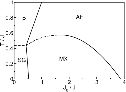
Figure 1: The zero-field phase diagram for $r=3$ showing the paramagnetic (P), antiferromagnetic (AF), spin-glass (SG) and mixed (MX) or glassy antiferromagnetic phases. Solid lines indicate continuous transitions and the dashed lines D1RSB transitions.

4 The phase diagrams

We present the results only for $r=3$ since the the general features of the phase diagrams do not depend sensitively on $r$.

4.1 Results for $H=0$

The zero-field phase diagram is shown in Figure 1. We found four phases which meet at a multicritical point: the paramagnetic (P) phase, antiferromagnetic (AF) phase, spin glass (SG) phase and mixed (MX) phase (or glassy antiferromagnetic phase). The P and AF phases show no replica symmetry breaking and are described by the RS solution. The P phase is characterised by the order parameters

$$m_{A}=m_{B}=0,\qquad q_{A}=q_{B}=0,$$ (25)

and the AF phase by

$$m_{A}=-m_{B}\neq 0,\qquad q_{A}=q_{B}.$$ (26)

The SG and MX phases present replica symmetry breaking and are described by 1RSB solution. The SG phase is characterised by the order parameters

$$m_{A}=m_{B}=0,\qquad q_{0A}=q_{0B}<q_{1A}=q_{1B},\qquad 0<x<1,$$ (27)

and the MX phase by

$$m_{A}=-m_{B}\neq 0,\qquad q_{0A}=q_{0B}<q_{1A}=q_{1B},\qquad 0<x<1.$$ (28)

If we make the substitutions $m_{A}\rightarrow m$, $m_{B}\rightarrow-m$, $q_{0A},q_{0B}\rightarrow q_{0}$ and $q_{1A},q_{1B}\rightarrow q_{1}$ in (19-24), these equations become identical to those of one-sublattice $p$-spin spherical model with ferromagnetic interactions $-J_{0}$ and $p=2r$ [8]. Thus in the absence of an external field the results of the one-sublattice model can be translated to the two-sublattice model simply by exchanging the ferromagnetic and antiferromagnetic orderings. The P-AF and the SG-MX transitions are continuous and are characterised by the appearance of spontaneous sublattice magnetisations $m_{A}=-m_{B}\neq 0$ in the AF and MX phases. The P-SG and the AF-MX transitions are characterised by the emergence of 1RSB solution with higher free energy than the RS solution in the SG and MX phases. In the SG to the P transition $x\rightarrow 1$ and $q_{1I}-q_{0I}$ vanishes discontinuously. Thus there is a discontinuous one-step replica-symmetry-breaking (D1RSB) transition. The AF-MX transition is also a D1RSB transition to the left of the maximum in the boundary of MX phase, but to the right of the maximum $q_{0A}=q_{0B}$ and $q_{1A}=q_{1B}$ merge continuously at the transition with $x<1$. Thus there is a continuous one-step replica-symmetry-breaking (C1RSB) transition. We observe that although the spin-glass order parameters change discontinuously across the D1RSB transition, thermodynamically it is a continuous transition [5, 7].

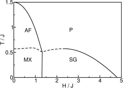
Figure 2: The field-temperature phase diagram of the model for $J_{0}/J=1.5$ and $r=3$. The solid lines represent continuous transitions and the dashed lines D1RSB transitions.

4.2 Results for $H>0$

The phase diagram of the model in a uniform external field is shown in Figure 2 for $J_{0}/J=1.5$ and $r=3$. We again found four phases that meet at a multicritical point. The P and AF phases show no replica symmetry breaking and are described by the RS solution. The P phase is characterised by the order parameters

$$m_{A}=m_{B}\neq 0,\qquad q_{A}=q_{B},$$ (29)

and the AF phase by

$$m_{A}\neq m_{B},\qquad q_{A}\neq q_{B}.$$ (30)

The SG and MX phases present replica symmetry breaking and are described by 1RSB solution. The SG phase is characterised by the order parameters

$$m_{A}=m_{B}\neq 0,\qquad q_{0A}=q_{0B},\qquad q_{1A}=q_{1B},\qquad 0<x<1,$$ (31)

and the MX phase by

$$m_{A}\neq m_{B},\qquad q_{0A}\neq q_{0B},\qquad q_{1A}\neq q_{1B},\qquad 0<x<1.$$ (32)

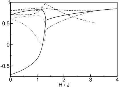
Figure 3: The order parameters as functions of the magnetic field for $r=3$, $J_{0}/J=1.5$ and $T/J=0.5$. The full lines represent $m_{A}$ and $m_{B}$, the dotted lines $q_{0A}$ and $q_{0B}$, the dashed lines $q_{1A}$ and $q_{1B}$, and the dash-dotted line represents $x$.

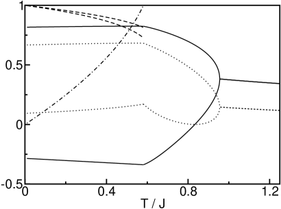
Figure 4: The order parameters as functions of the temperature for $r=3$, $J_{0}/J=1.5$ and $H/J=1$. The full lines represent $m_{A}$ and $m_{B}$, the dotted lines $q_{0A}$ and $q_{0B}$, the dashed lines $q_{1A}$ and $q_{1B}$, and the dash-dotted line represents $x$.

The order parameters as functions of the external field is plotted in Figure 3 for $r=3$, $J_{0}/J=1.5$ and $T/J=0.5$, when the system undergoes transitions from MX to SG and from SG to P phases for increasing fields. The MX-SG transition takes place at $H/J=1.32$. At this transition the sublattice order parameters $m_{A}$ and $m_{B}$, $q_{0A}$ and $q_{0B}$, and $q_{1A}$ and $q_{1B}$ become identical with $x<1$, implying a continuous transition between RSB phases. At the SG-P transition at $H/J=3.15$ the order parameters $q_{0A}=q_{0B}$ and $q_{1A}=q_{1B}$ merge continuously with $x<1$, indicating a C1RSB transition.

Figure 4 shows the order parameters as functions of the temperature for $r=3$, $J_{0}/J=1.5$ and $H/J=1$, when the system undergoes transitions from MX to AF and from AF to P phases for increasing temperatures. The MX-AF transition takes place at $T/J=0.58$. At this transition the sublattice magnetisations $m_{A}$ and $m_{B}$ meet continuously. However $q_{0B}$ and $q_{1B}$ do not merge continuously with $q_{1A}$ and $q_{1B}$. Also $x\rightarrow 1$ at the transition, which indicates a D1RSB transition. The AF-P transition at $T/J=0.95$ is a conventional continuous transition between RS phases.

Figure 5: Free energy per spin as a function of temperature for $H/J=1.0$, $J_{0}/J=1.5$ and $r=3$. The solid and dashed lines represent the 1RSB and RS solutions respectively.

The free energies of the RS and 1RSB solutions for $r=3$, $J_{0}/J=1.5$ and $H/J=1$ are shown in Figure 5 across the MX-AF transition. We observe that in the MX phase the free energy of the 1RSB solution is higher than the RS solution. A similar behaviour was also found in the one-sublattice model [7]. In the replica approach this indicates that we must choose the 1RSB rather than the RS solution [1].

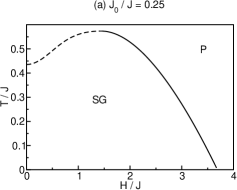
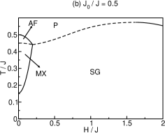
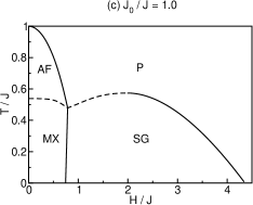
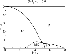
Figure 6: The field-temperature phase diagrams for various values of $J_{0}$. The full line represent continuous transitions while the dashed and dotted lines represent D1RSB transitions.

Figures 6(a)-(f) show the evolution of the field-temperature phase diagrams for increasing values of the antiferromagnetic coupling $J_{0}$. In Figure 6(a) for $J_{0}/J=0.25$ only the SG and the P phases are present. The P-SG boundary has a maximum. It is a D1RSB transition to the left of maximum and C1RSB transition to the right. This feature of P-SG transition is common to all the subsequent phase diagrams. In Figure 6(b) for $J_{0}/J=0.5$ the AF and MX phases are present for small magnetic fields. The P-AF and MX-SG transitions are always continuous. The MX-AF transition is of D1RSB type. In Figure 6(c) for $J_{0}/J=1.0$ the MX phase extends to zero temperature. In Figure 6(d) the AF-MX boundary exhibits a C1RSB transition in the low field side. This feature of the AF-MX transition which starts at $J_{0}/J=1.72$ is common to all subsequent phase diagrams. In Figure 6(e) for $J_{0}/J=3.5$ the MX phase is no longer present at zero field. Finally, in Figure 6(f) the D1RSB transition line has disappeared in the P-SG boundary, and only the C1RSB transition line remains. Also the the D1RSB transition in the MX-AF boundary becomes again a C1RSB transition before reaching the multicritical point.

5 Conclusions

We have studied the thermodynamic properties and phase diagrams of a $r$-spin antiferromagnetic spherical spin-glass model using the replica method. For this class of models the first step in the replica symmetry breaking is sufficient [7]. The model is a two-sublattice version of the $p$-spin ferromagnetic spherical spin-glass model [8]. The two models become essentially identical in their properties in the absence of an external field if the roles of the ferromagnetic and the antiferromagnetic orderings are exchanged. The model can also be considered as a spherical version of the antiferromagnetic SK model [14, 15, 16] and the antiferromagnetic REM model [17].

We have presented a detailed numerical study for the representative case $r=3$. The phase diagrams comprise the paramagnetic (P) phase, the antiferromagnetic (AF) phase, the spin-glass (SG) phase and mixed (MX) or glassy antiferromagnetic phases. All the transitions between these phases are continuous in the thermodynamic sense. However the spin-glass order parameters may change continuously (C1RSB) or discontinuously (D1RSB) in the SG-P and MX-AF transitions.

Previous studies of the same problem in antiferromagnetic SK model [14, 15, 16] and the antiferromagnetic REM model [17] have yielded qualitatively similar phase diagrams. However the P-SG and AF-MX transitions are of continuous $\infty$RSB type in the antiferromagnetic SK model [14, 15, 16] and of continuous C1RSB type in the REM model [17].

References

References

- [1] Mezard M, Parisi G and Virasoro M A 1987 Spin Glass Theory and Beyond (Singapore: World Scientific)
- [2] Nishimori H 2001 Statistical Physics of Spin Glasses and Information Processing (Oxford: Oxford University Press)
- [3] Sherrington D and Kirkpatrick S 1975 Phys. Rev. Lett. 26, 1792-6
- [4] Parisi G 1980 J. Phys. A: Math. Gen. 13, 1887-95
- [5] Gross D J and Mezard M 1984 Nucl. Phys. B 240, 431-52
- [6] Derrida B 1980 Phys. Rev. Lett. 45, 79-82
- [7] Crisanti A and Sommers H-J 1992 Z. Phys. B 87, 341-54
- [8] Hertz J A, Sherrington D and Nieuwenhuizen T M 1999 Phys. Rev. E 60, R2460-3
- [9] Bertrand D, Fert A R, Schmidt M C, Bensamka F and Legrand S 1982 J. Phys. C: Solid State Phys. 15, L883-8
- [10] Wong P Z, Vonmolnar S, Palstra T T M, Mydosh J A, Yoshizawa H, Shapiro S M and Ito A 1985 Phys. Rev. Lett. 55, 2043-6
- [11] Wong P Z, Yoshizawa H and Shapiro S M 1985 J. Applied Phys. 57, 3462-4
- [12] Yoshizawa H, Mitsuda S, Aruga H and Ito A 1987 Phys. Rev. Lett. 59, 2364-7
- [13] Yoshizawa H, Mori H, Kawano H, Aruga-Katori H, Mitsuda S and Ito A 1994 J. Phys. Soc. Japan 63, 3145-57
- [14] Korenblit I Y and Shender E F 1985 Sov. Phys. JETP 62, 1785-95
- [15] Fyodorov Y V, Korenblit I Y and Shender E F 1987 J. Phys. C: Solid State Phys. 20, 1835-9
- [16] Takayama H 1988 Prog. Theor. Phys. 80, 827-39
- [17] de Almeida J R L 1998 Phys. Stat. Sol. (b) 209, 153-9
- [18] Montenegro F C, Lima K A, Torkachvili M S and Lacerda A 1998 J. Magn. Magn. Mater. 145, 177-81