Scalar, vectorial and tensorial damage parameters from the mesoscopic background

Abstract.

In the mesoscopic theory a distribution of different crack sizes and crack orientations is introduced. A scalar damage parameter, a second order damage tensor and a vectorial damage parameter are defined in terms of this distribution function. As an example of a constitutive quantity the free energy density is given as a function of the damage tensor. This equation is reduced in the uniaxial case to a function of the damage vector and in case of a special geometry to a function of the scalar damage parameter.

1. Introduction

1.1. Phenomenological definitions of damage parameters

Numerous damage models have incorporated scalar, vectorial or tensorial damage variables that can be characterized at the macro-scale, for example, by the change in compliance. A scalar damage parameter has been introduced [1, 2, 3, 4] to account for the decrease in the stiffness of the material with progressing damage. Two scalar damage parameters have been proposed [5] to account independently for the change in hydrostatic energy and the remaining part of the elastic energy with increasing damage. A different reason for introducing two scalar damage parameters was in [6] to account for healing of cracks under compression. In composites and fiber reinforced materials it is reasonable to introduce independent scalar order parameters for the prescribed directions, given by the fiber orientation.

A second order damage tensor has been defined [7], accounting for the reduction of the effective surface area, which transmits forces. The resulting effective stress is expressed in terms of the damage tensor [7]. For definitions of a second order damage tensor see also [3, 8, 9, 10, 11]. For parallel microcracks a second order damage tensor has been associated with the dyadic product of crack orientation with itself times a scalar parameter [12]. This definition coincides with our definition from the mesoscopic point of view in the special case of parallel microcracks.

A fourth order damage tensor has been introduced. It can be understood as mapping the elastic tensor of the virgin material to the elastic tensor of the damaged material, or as mapping the respective stress tensors. For a summary of damage parameters of different orders see also [13, 14].

For a constitutive theory of damaged materials with a thermodynamic background see [15, 16]. A thermodynamic theory of damage, including the interpretation of failure as loss of thermodynamic stability, can be found in [17]. For a comparison to experimental results see [18].

An alternative choice of damage variable is one that incorporates salient aspects of damage morphology in its definition. Such “micro-mechanically- inspired” damage models involving scalar, tensor, or “Fabric tensor” representations of damage have been introduced in the study of heterogeneous materials containing voids or various crack-like surface discontinuities [19, 20, 21, 22, 23, 24].

Our aim here is to show how damage parameters of different tensor order can be defined from the mesoscopic background. The different damage parameters correspond to different levels of macroscopic approximation of the mesoscopic distribution of crack sizes and orientations. As it has been shown in [25, 26] in the case of a scalar damage parameter, the mesoscopic theory leads not only to the definition of damage parameters, but also to equations of motion for them. On the example of the free energy density we will show the general form of a constitutive equation for the different choices of a damage parameter. In the case of a rotation symmetry of crack orientations, the different forms of constitutive equation can be reduced to a form with two scalar parameters: the average crack size and a scalar orientational order parameter.

1.2. Mesoscopic theory of complex materials and application to material damage

The mesoscopic theory has been developed in order to deal with complex materials within continuum mechanics [27]. The idea is to enlarge the domain of the field quantities by an additional variable, characterizing the internal degree of freedom connected with the internal structure of the material. In a simple model the micro-crack is described as a flat, rotation symmetric surface, a so called penny shaped crack. In addition we make here the following simplifying assumptions:

1. The diameter of the cracks is much smaller than the linear dimension of the continuum element. Under this assumption the cracks can be treated as an internal structure of the continuum element. The cracks are assumed small enough that there is a whole distribution of crack sizes and orientations in the volume element.

2. The cracks are fixed to the material. Therefore their motion is coupled to the motion of representative volume elements.

3. The cracks cannot rotate independently of the material, i. e. the rotation velocity is determined by the antisymmetric part of the time derivative of the deformation gradient of the surrounding material.

4. The number of cracks is fixed, there is no production of cracks, but very short cracks are preexisting in the virgin material.

5. The cracks cannot decrease area, but can only enlarge, meaning that cracks cannot heal.

To summarize our model the micro-crack is characterized by a unit vector $n$ representing the orientation of the surface normal and by the radius $l$ of the spherical crack surface. These parameters will be taken as the additional variables in the mesoscopic theory.

Beyond the use of additional variables the mesoscopic concept introduces a statistical element, the so-called mesoscopic distribution function. In our case this is a distribution of crack lengths and orientations in the continuum element at position $x$ and time $t$, called here crack distribution function (CDF). The distribution function is the probability density of finding a crack of length $l$ and orientation $n$ in the continuum element. The elements are material elements, including the same material and the same cracks for all times. Macroscopic quantities are calculated from mesoscopic ones as averages over crack sizes and crack orientations.

1.3. Mesoscopic balance equations

Field quantities such as mass density, momentum density, angular momentum density, and energy density are defined on the mesoscopic space. For distinguishing these fields from the macroscopic ones we add the word “mesoscopic“. In addition to mass density we introduce the crack number density $N$ as the density of an extensive quantity. The mesoscopic crack number density $N(l,\mbox{\boldmath{$n$}},\mbox{\boldmath{$x$}},t)$ is the number density, counting only cracks of length $l$ and orientation $n$.

Balance of crack number
In our model the cracks move together with the material element. Therefore their flux is the convective flux, having a part in position space, a part in orientation space, and a part in the length interval. There is no production and no supply of crack number. Therefore we have for the crack number density $N$:

(1.1) $$\frac{\partial}{\partial t}N(\cdot)+\nabla_{x}\cdot\{N(\cdot)\mbox{\boldmath{$v$}}(\mbox{\boldmath{$x$}},t)\}+\nabla_{n}\cdot\{N(\cdot)\mbox{\boldmath{$u$}}(\cdot)\}+\frac{1}{l^{2}}\frac{\partial}{\partial l}\left(l^{2}\dot{l}N(\cdot)\right)\ =\ 0.$$

We have used spherical coordinates for the mesoscopic variables crack length $l\in[0,\infty]$ and crack orientation $\mbox{\boldmath{$n$}}\in S^{2}$, and we represent the divergence with respect to the mesoscopic variables in spherical coordinates. $\nabla_{n}$ denotes the covariant derivative on the unit sphere. $v$ is the material velocity. In our model all cracks within the continuum element move with this velocity. $\mbox{\boldmath{$u$}}(\cdot)=\dot{\mbox{\boldmath{$n$}}}$ is the orientation change velocity, which is not the same for all cracks in the continuum element. It is related to the angular velocity $\mbox{\boldmath{$\omega$}}(\mbox{\boldmath{$x$}},t)$ by the relation

(1.2) $$\mbox{\boldmath{$u$}}(\cdot)=\mbox{\boldmath{$\omega$}}\times\mbox{\boldmath{$n$}}$$

This angular velocity is the same for all cracks in the element. It is determined by the rotation of the surrounding material.

1.4. Definition of the distribution function and equation of motion

Due to its definition as probability density the distribution function is the number fraction

(1.3) $$f(l,\mbox{\boldmath{$n$}},\mbox{\boldmath{$x$}},t)=\frac{N(l,\mbox{\boldmath{$n$}},\mbox{\boldmath{$x$}},t)}{N(\mbox{\boldmath$x$},t)}\quad,$$

in volume elements, where the number density $N(\mbox{\boldmath{$x$}},t)$ is non-zero. Here $N(\mbox{\boldmath$x$},t)$ is the macroscopic number density of cracks of any length and orientation. As the distribution function in equation (1.3) is not well defined if $N(\mbox{\boldmath$x$},t)=0$, we define in addition that in this case $f(l,\mbox{\boldmath{$n$}},\mbox{\boldmath{$x$}},t)=0$. As there is no creation of cracks in our model the distribution function will be zero for all times in these volume elements. In all other volume elements with a nonzero crack number it is normalized

(1.4) $$\int_{0}^{\infty}\int_{S^{2}}f(l,\mbox{\boldmath{$n$}},\mbox{\boldmath{$x$}},t)l^{2}d^{2}ndl=1\quad.$$

With respect to crack length it is supposed that the distribution function has a compact support, meaning that in a sample there cannot exist cracks larger than the sample size.

We obtain from the mesoscopic balance of crack number density a balance of the CDF $f(l,\mbox{\boldmath{$n$}},\mbox{\boldmath{$x$}},t)$, by inserting its definition:

$$\frac{\partial}{\partial t}f(l,\mbox{\boldmath{$n$}},\mbox{\boldmath{$x$}},t)+\nabla_{x}\cdot\left(\mbox{\boldmath{$v$}}(\mbox{\boldmath{$x$}},t)f(l,\mbox{\boldmath{$n$}},\mbox{\boldmath{$x$}},t)\right)+$$

(1.5) $$\nabla_{n}\cdot\left(\mbox{\boldmath{$u$}}(\mbox{\boldmath{$x$}},t)f(l,\mbox{\boldmath{$n$}},\mbox{\boldmath{$x$}},t)\right)+\frac{1}{l^{2}}\frac{\partial}{\partial l}\left(l^{2}\dot{l}f(l,\mbox{\boldmath{$n$}},\mbox{\boldmath{$x$}},t)\right)=0.$$

The right hand side is equal to zero, as for the co-moving observer the total number of cracks in a volume element does not change in time.

A growth law for the single crack $\dot{l}$ is needed in equation (1.5). For example the Rice-Griffith dynamics, which is motivated from macroscopic thermodynamic considerations, has been applied.

In [28] the mesoscopic theory has been specialized to damaged material with penny shaped cracks. The balance equations and the differential equation for the crack size distribution function have been derived. With Rice-Griffith differential equation for the size of a single crack, the time evolution of the whole distribution of cracks under load has been investigated, as well as the evolution of the average crack size [29]. In [30] two different growth laws for the single crack under load have been considered. Finally, the dynamics of a second order damage tensor has been derived in [26] under the assumption of a simplified single crack growth law under an effective stress.

2. Mesoscopic definitions of damage parameters of different orders

Definitions of a scalar damage parameter, a vectorial parameter and a damage tensor are given, based on the mesoscopic distribution function. A scalar damage parameter is the average crack length. The crack growth introduces an anisotropy into the material. In order to describe this anisotropy, it is necessary to define a vectorial or a tensorial damage parameter. Starting from the mesoscopic distribution function, the more natural way is to define a damage tensor of second order. The tensor character is introduced by the second moment of the distribution function with the crack orientation vector. A case of special interest is a distribution with a rotation symmetry, the uniaxial case. In this case the damage tensor can be expressed in terms of a scalar and a unit vector, which is the orientation of the rotation symmetry axis. In this case we can define easily a damage vector from the second order damage tensor. This damage vector has the orientation of the rotation symmetry axis. A representation of the second order damage tensor in the general case without rotation symmetry is also given. It is shown how a vectorial damage parameter can be defined in general without rotation symmetry in terms of eigenvectors of the damage tensor.

2.1. Damage parameter of second order

We define the second order damage tensor as the second orientational moment of the distribution function:

$$\mbox{\boldmath{$D$}}(\mbox{\boldmath{$x$}},t)=<l\hskip 1.99997pt\stackrel{{\scriptstyle\vrule width=0.2411pt,height=0.2411pt,depth=1.43161pt\hbox{\vrule width=9.24326pt,height=0.2411pt,depth=0.0pt}\vrule width=0.2411pt,height=0.2411pt,depth=1.43161pt}}{{\mbox{\boldmath{$n$}}\mbox{\boldmath{$n$}}}}\hskip 1.99997pt>=\int_{0}^{\infty}l\int_{S^{2}}f(l,\mbox{\boldmath{$n$}},\mbox{\boldmath{$x$}},t)\hskip 1.99997pt\stackrel{{\scriptstyle\vrule width=0.2411pt,height=0.2411pt,depth=1.43161pt\hbox{\vrule width=9.24326pt,height=0.2411pt,depth=0.0pt}\vrule width=0.2411pt,height=0.2411pt,depth=1.43161pt}}{{\mbox{\boldmath{$n$}}\mbox{\boldmath{$n$}}}}\hskip 1.99997ptd^{2}nl^{2}{\rm d}l$$

(2.6) $$=\int_{0}^{\infty}\int_{S^{2}}l^{3}\hskip 1.99997pt\stackrel{{\scriptstyle\vrule width=0.2411pt,height=0.2411pt,depth=1.43161pt\hbox{\vrule width=9.24326pt,height=0.2411pt,depth=0.0pt}\vrule width=0.2411pt,height=0.2411pt,depth=1.43161pt}}{{\mbox{\boldmath{$n$}}\mbox{\boldmath{$n$}}}}\hskip 1.99997ptf(l,\mbox{\boldmath{$n$}},\mbox{\boldmath{$x$}},t)d^{2}n{\rm d}l$$

$\hskip 1.99997pt\stackrel{{\scriptstyle\vrule width=0.2411pt,height=0.2411pt,depth=1.43161pt\hbox{\vrule width=9.24326pt,height=0.2411pt,depth=0.0pt}\vrule width=0.2411pt,height=0.2411pt,depth=1.43161pt}}{{\mbox{\boldmath{$n$}}\mbox{\boldmath{$n$}}}}\hskip 1.99997pt$ denotes the symmetric traceless part of the dyadic product, and $D$ is a second order symmetric traceless tensor.

This definition of the second order damage parameter accounts for the crack length distribution as well as for the orientation distribution. With an applied load the length distribution evolves in time. This shows up in the evolution of the scalar damage parameter as well as in the evolution of the tensor damage parameter. As in our model all cracks rotate together with the surrounding material, the time evolution of the orientation distribution is a rigid rotation on the unit sphere.

2.2. Vectorial damage parameter defined from the second order tensor

Due to the symmetry the second order tensor damage parameter $D$ has a spectral decomposition with orthogonal eigenvectors (unit vectors) $d$, $e$ and $f$, and eigenvalues $\delta$, $\epsilon$ and $\phi$:

(2.7) $$\mbox{\boldmath{$D$}}=\delta\mbox{\boldmath{$d$}}\mbox{\boldmath{$d$}}+\epsilon\mbox{\boldmath{$e$}}\mbox{\boldmath{$e$}}+\phi\mbox{\boldmath{$f$}}\mbox{\boldmath{$f$}}\ .$$

Because $D$ is traceless we have

(2.8) $$\delta+\epsilon+\phi=0\ .$$

Therefore, not all eigenvalues can have the same sign. The following cases concerning the signs of the eigenvalues are possible

1. One eigenvalue is positive and two eigenvalues are negative, for instance

   (2.9) $$\delta>0,\quad\epsilon<0,\quad\Phi<0\ .$$

   In this case we chose the eigenvector (here $d$) corresponding to the single positive eigenvalue as the unit vector defining the orientation of the vector damage parameter.

2. One eigenvalue is negative and two eigenvalues are positive, for instance

   (2.10) $$\delta>0,\quad\epsilon>0,\quad\Phi<0\ .$$

   In this case we chose the eigenvector (here $f$) corresponding to the single negative eigenvalue as the unit vector defining the orientation of the vector damage parameter.

3. All eigenvalues are zero:

   (2.11) $$\delta=0,\quad\epsilon=0,\quad\phi=0\ .$$

   In this case $\mbox{\boldmath{$D$}}=0$ and we have an isotropic orientation distribution. In this case no vector damage parameter can be defined.

4. One eigenvalue is zero, and the two others have opposite sign, for instance:

   (2.12) $$\delta=0,\quad\epsilon>0,\quad\phi=-\epsilon<0\ .$$

   In this very special case we could define a vector damage parameter, having the orientation of the wedge-product of the two eigenvectors.

The length of the damage vector can be defined as the absolute value of the corresponding eigenvalue.

The definition of the damage vector in terms of an eigenvector naturally leads to the symmetry of an orientation, namely the damage vector and the reversed one cannot be distinguished.

2.3. Special case of uniaxial distribution function

If there exists a rotation symmetry axis of the distribution function, two eigenvalues coincide, either the two positive ones, or the two negative ones. In both cases the tensor damage parameter is of the form:

$$\mbox{\boldmath{$D$}}=\langle lS(l)\rangle\hskip 1.99997pt\stackrel{{\scriptstyle\vrule width=0.2411pt,height=0.2411pt,depth=1.43161pt\hbox{\vrule width=8.12677pt,height=0.2411pt,depth=0.0pt}\vrule width=0.2411pt,height=0.2411pt,depth=1.43161pt}}{{\mbox{\boldmath{$d$}}\mbox{\boldmath{$d$}}}}\hskip 1.99997pt=\langle lS(l)\rangle\left(\mbox{\boldmath{$d$}}\mbox{\boldmath{$d$}}-\frac{1}{3}\mbox{\boldmath{$1$}}\right)$$

(2.13) $$=\langle lS(l)\rangle\left(\mbox{\boldmath{$d$}}\mbox{\boldmath{$d$}}-\frac{1}{3}\left(\mbox{\boldmath{$d$}}\mbox{\boldmath{$d$}}+\mbox{\boldmath{$e$}}\mbox{\boldmath{$e$}}+\mbox{\boldmath{$f$}}\mbox{\boldmath{$f$}}\right)\right)$$

with the unit tensor $1$ and a scalar parameter $S$, denoted as scalar orientational order parameter. The unit vector $d$ is the orientation of the rotation symmetry axis. $S(l)$ is a measure of the degree of parallel order of the cracks. It is zero if the orientations are distributed isotropically and has the value 1 in the case that all cracks are oriented parallel. The orientational order can be different for different crack sizes, therefore $S$ is a function of crack radius $l$. The average $\langle\quad\rangle$ here is the average over all crack lengths:

(2.14) $$\langle lS(l)\rangle=\int_{0}^{\infty}f(l,\mbox{\boldmath{$x$}},t)lS(l)l^{2}dl\ .$$

For the eigenvalues this corresponds to

(2.15) $$\delta=\langle lS(l)\rangle\left(1-\frac{1}{3}\right)=\frac{2}{3}\langle lS(l)\rangle$$

(2.16) $$\epsilon=-\frac{1}{3}\langle lS(l)\rangle$$

(2.17) $$\phi=-\frac{1}{3}\langle lS(l)\rangle\ .$$

For positive values of $S$ we have one positive eigenvalue and two negative ones. For negative values of $S$ two eigenvalues are positive and one is negative. In both cases the definition of the vector damage parameter given in the section above leads to the eigenvector $d$ as the orientation of the damage vector. In case of rotation symmetric orientation distributions this is the orientation of the rotation symmetry axis. The case of positive values of $S$ corresponds to a distribution, where the crack-normals are more or less parallel to the rotation symmetry axis. For negative values of $S$ crack orientations are concentrated in a plane perpendicular to the rotation symmetry axis (see figure 1).

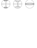
Figure 1. Different cases of rotation symmetric crack orientation distributions, corresponding to different values of the orientational order parameter.

For the damage vector we find in the uniaxial case:

(2.18) $$\vec{D}=\frac{2}{3}\langle lS(l)\rangle\mbox{\boldmath{$d$}}\ .$$

It depends on the degree of orientational order and on the average crack length.

2.4. Case of small deviation of the distribution function from rotation symmetry

If the deviation of the orientation distribution from rotation symmetry is small, the two eigenvalues of equal sign differ only by a small amount $s$, and the damage tensor is of the form:

(2.19) $$\mbox{\boldmath{$D$}}=\left(\frac{2}{3}\langle S(l)l\rangle\mbox{\boldmath{$d$}}\mbox{\boldmath{$d$}}+\left(-\frac{1}{3}\langle(S(l)-s(l))l\rangle\right)\mbox{\boldmath{$e$}}\mbox{\boldmath{$e$}}+\left(-\frac{1}{3}\langle(S(l)-s(l))l\rangle\right)\mbox{\boldmath{$f$}}\mbox{\boldmath{$f$}}\right)\ .$$

In this case we can still define the damage vector the same way as in the uniaxial case:

(2.20) $$\vec{D}=\frac{2}{3}\langle lS(l)\rangle\mbox{\boldmath{$d$}}\ .$$

The scalar order parameter $S$ is a measure of the degree of order and the biaxiality parameter $s$ is a measure of the deviation of the orientation distribution from rotation symmetry.

2.5. Scalar damage parameters

One possible definition of a scalar damage parameter is the average crack length:

(2.21) $$D=\int_{0}^{\infty}lf(l,\mbox{\boldmath{$x$}},t)l^{2}dl\ .$$

In the rotation symmetric case another scalar measure of damage is

(2.22) $$D_{S}=\langle lS(l)\rangle=\int_{0}^{\infty}lS(l)f(l,\mbox{\boldmath{$x$}},t)l^{2}dl\ .$$

It is the average crack radius, projected onto the plane perpendicular to the rotation symmetry axis. This is the quantity relevant for describing the progressive damage under external load in case of an anisotropic crack distribution.

3. Examples of constitutive functions for the different damage descriptions

In this section we will show on the example of the free energy density, how the constitutive equation reduces from a representation in terms of the second order damage tensor to one in terms of a vector, or a scalar, respectively.

We will assume, that constitutive quantities depend on the equilibrium variables strain and temperature and in addition on the damage parameter. The temperature dependence will not be denoted explicitly, as it is a scalar quantity. All material coefficients may depend on temperature.

3.1. Free energy as a function of strain and damage in case of a second order damage tensor

The most general polynomial form of the energy density up to second order in each variable is given by a representation theorem [31, 32]:

$$F(\mbox{\boldmath{$\epsilon$}},\mbox{\boldmath{$D$}},D)=a_{2}D+\frac{b_{1}}{2}D^{2}+b_{2}tr(\mbox{\boldmath{$D$}}\cdot\mbox{\boldmath{$D$}})$$

$$+\left(a_{1}+b_{4}D+c_{2}D^{2}+c_{5}tr(\mbox{\boldmath{$D$}}\cdot\mbox{\boldmath{$D$}})\right)tr(\mbox{\boldmath{$\epsilon$}})$$

$$\left(b_{3}+c_{4}D\right)tr(\mbox{\boldmath{$\epsilon$}}\cdot\mbox{\boldmath{$D$}})+c_{8}tr(\mbox{\boldmath{$D$}}\cdot\mbox{\boldmath{$D$}}\cdot\mbox{\boldmath{$\epsilon$}})$$

$$+\left(\frac{\lambda}{2}+c_{1}D+d_{1}D^{2}+d_{3}tr(\mbox{\boldmath{$D$}}\cdot\mbox{\boldmath{$D$}})\right)\left(tr(\mbox{\boldmath{$\epsilon$}})\right)^{2}$$

$$+\left(\mu+c_{6}D+d_{2}D^{2}+d_{4}tr(\mbox{\boldmath{$D$}}\cdot\mbox{\boldmath{$D$}})\right)tr(\mbox{\boldmath{$\epsilon$}}\cdot\mbox{\boldmath{$\epsilon$}})$$

$$+\left(c_{3}tr(\mbox{\boldmath{$\epsilon$}})+d_{5}tr(\mbox{\boldmath{$\epsilon$}}\cdot\mbox{\boldmath{$D$}})+d_{6}tr(\mbox{\boldmath{$\epsilon$}})D\right)tr(\mbox{\boldmath{$\epsilon$}}\cdot\mbox{\boldmath{$D$}})$$

$$+\left(c_{7}+d_{8}D\right)tr(\mbox{\boldmath{$\epsilon$}}\cdot\mbox{\boldmath{$\epsilon$}}\cdot\mbox{\boldmath{$D$}})+d_{7}tr(\mbox{\boldmath{$\epsilon$}})tr(\mbox{\boldmath{$D$}}\cdot\mbox{\boldmath{$D$}}\cdot\mbox{\boldmath{$\epsilon$}})$$

(3.23) $$+d_{9}tr(\mbox{\boldmath{$D$}}\cdot\mbox{\boldmath{$D$}}\cdot\mbox{\boldmath{$\epsilon$}}\cdot\mbox{\boldmath{$\epsilon$}})$$

This form is the simplest and natural extension of linear elasticity considering the damage. The coefficients still can be arbitrary functions of temperature.

In the case of rotation symmetry we have:

(3.24) $$\mbox{\boldmath{$D$}}=D_{S}\hskip 1.99997pt\stackrel{{\scriptstyle\vrule width=0.2411pt,height=0.2411pt,depth=1.43161pt\hbox{\vrule width=8.12677pt,height=0.2411pt,depth=0.0pt}\vrule width=0.2411pt,height=0.2411pt,depth=1.43161pt}}{{\mbox{\boldmath{$d$}}\mbox{\boldmath{$d$}}}}\hskip 1.99997pt$$

and the scalar products can be calculated as:

$$\mbox{\boldmath{$D$}}\cdot\mbox{\boldmath{$D$}}=D_{S}^{2}\hskip 1.99997pt\stackrel{{\scriptstyle\vrule width=0.2411pt,height=0.2411pt,depth=1.43161pt\hbox{\vrule width=8.12677pt,height=0.2411pt,depth=0.0pt}\vrule width=0.2411pt,height=0.2411pt,depth=1.43161pt}}{{\mbox{\boldmath{$d$}}\mbox{\boldmath{$d$}}}}\hskip 1.99997pt\cdot\hskip 1.99997pt\stackrel{{\scriptstyle\vrule width=0.2411pt,height=0.2411pt,depth=1.43161pt\hbox{\vrule width=8.12677pt,height=0.2411pt,depth=0.0pt}\vrule width=0.2411pt,height=0.2411pt,depth=1.43161pt}}{{\mbox{\boldmath{$d$}}\mbox{\boldmath{$d$}}}}\hskip 1.99997pt$$

(3.25) $$=D_{S}^{2}\left(\mbox{\boldmath{$d$}}\mbox{\boldmath{$d$}}-\frac{1}{3}\mbox{\boldmath{$1$}}\right)\cdot\left(\mbox{\boldmath{$d$}}\mbox{\boldmath{$d$}}-\frac{1}{3}\mbox{\boldmath{$1$}}\right)=D_{S}^{2}\left(\frac{1}{3}\mbox{\boldmath{$d$}}\mbox{\boldmath{$d$}}+\frac{1}{9}\mbox{\boldmath{$1$}}\right)$$

and

(3.26) $$tr(\mbox{\boldmath{$D$}}\cdot\mbox{\boldmath{$D$}})=\frac{2}{3}D_{S}^{2}$$

The expression for the free energy simplifies to:

$$F(\mbox{\boldmath{$\epsilon$}},D_{S},\mbox{\boldmath{$d$}},D)=a_{2}D+\frac{b_{1}}{2}D^{2}+\frac{2}{3}b_{2}D_{S}^{2}+$$

$$tr(\mbox{\boldmath{$\epsilon$}})\left(a_{1}+b_{4}D+c_{2}D^{2}-\frac{1}{3}b_{3}D_{S}-\frac{1}{3}c_{4}DD_{S}+(\frac{2}{3}c_{5}+\frac{1}{9}c_{8})^{2}D_{S}^{2}\right)$$

$$+(tr\mbox{\boldmath{$\epsilon$}})^{2}\left(\frac{1}{2}\lambda+c_{1}D+d_{1}D^{2}-\frac{1}{3}c_{3}D_{S}-\frac{1}{3}d_{6}DD_{S}\right.$$

$$\left.+(\frac{2}{3}d_{3}+\frac{1}{9}d_{5}+\frac{1}{9}d_{7})D_{S}^{2}\right)+$$

$$tr(\mbox{\boldmath{$\epsilon$}}\cdot\mbox{\boldmath{$\epsilon$}})\left(\mu+c_{6}D+d_{2}D^{2}-\frac{1}{3}c_{7}D_{S}-\frac{1}{3}c_{8}DD_{S}+(\frac{2}{3}d_{4}+\frac{1}{9}d_{9})D_{S}^{2}\right)$$

$$+\mbox{\boldmath{$\epsilon$}}:\mbox{\boldmath{$d$}}\mbox{\boldmath{$d$}}\left(b_{3}D_{S}+c_{4}DD_{S}+\frac{1}{3}c_{8}D_{S}^{2}\right)+\left(\mbox{\boldmath{$\epsilon$}}:\mbox{\boldmath{$d$}}\mbox{\boldmath{$d$}}\right)^{2}d_{5}D_{S}$$

$$+(tr\mbox{\boldmath{$\epsilon$}})\mbox{\boldmath{$\epsilon$}}:\mbox{\boldmath{$d$}}\mbox{\boldmath{$d$}}\left((d_{5}+c_{3})D_{S}+d_{6}DD_{S}+\frac{1}{3}d_{7}tr\mbox{\boldmath{$\epsilon$}}D_{S}^{2}\right)$$

(3.27) $$+\mbox{\boldmath{$d$}}\cdot\mbox{\boldmath{$\epsilon$}}\cdot\mbox{\boldmath{$\epsilon$}}\cdot\mbox{\boldmath{$d$}}\left(c_{7}D_{S}+d_{8}DD_{S}+\frac{1}{3}d_{9}D_{S}^{2}\right)$$

The free energy density is expressed here in terms of the vector $d$ (the rotation symmetry axis) and the scalar damage parameter $D_{S}$.

3.2. Special case of uniaxial strain in the z-direction and symmetry axis of the distribution in the same direction

This situation occurs (approximately) in a uniaxial tension experiment (see figure 2).

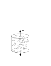
Figure 2. Schematic view of an experiment with uniaxial loading.

The assumption that in all volume elements the CDF is rotation symmetric with the $z$-direction as symmetry axis is an approximation, valid for small deformations. In case of large deformations, the rotation of the volume element cannot be neglected, and the cracks rotate with the material element. This leads to a rotation of the symmetry axis of the orientation distribution function in the volume element, which depends on the position of the volume element. The (local) symmetry axis of the CDF does not coincide with the direction of the applied strain anymore.

In the geometry with the global rotation symmetry around the z-axis the only interesting components of tensors are the z-z-components and traces. For the strain and the damage vector we have:

(3.28) $$\mbox{\boldmath{$\epsilon$}}=\epsilon_{zz}\mbox{\boldmath{$e$}}_{z}\mbox{\boldmath{$e$}}_{z}=:\epsilon\mbox{\boldmath{$e$}}_{z}\mbox{\boldmath{$e$}}_{z}$$

(3.29) $$\mbox{\boldmath{$d$}}=\mbox{\boldmath{$e$}}_{z}$$

and the free energy density reduces to a function of three scalar quantities $\epsilon,D,D_{S}$. $D$ is the average crack length (in any direction) and $D_{S}$ is a measure of the anisotropy of the average crack length distribution in the z-direction and orthogonal to it.

$$F(\epsilon,D_{S},D)=a_{2}D+\frac{b_{1}}{2}D^{2}+\frac{2}{3}b_{2}D_{S}^{2}$$

$$+\epsilon\left(a_{1}+b_{4}D+c_{2}D^{2}+\left(\frac{2}{3}b_{3}+\frac{2}{3}c_{4}D\right)D_{S}+\left(\frac{2}{3}c_{5}+\frac{4}{9}c_{8}\right)D_{S}^{2}\right)$$

$$\epsilon^{2}\left(\frac{\lambda}{2}+\mu+\left(c_{1}+c_{6}\right)D+\left(d_{1}+d_{2}\right)D^{2}\right.$$

$$D_{S}\left(\frac{2}{3}c_{3}+\frac{2}{3}c_{7}+D\left(\frac{2}{3}d_{6}+\frac{2}{3}d_{8}\right)\right)$$

(3.30) $$\left.+D_{S}^{2}\left(\frac{2}{3}d_{3}+\frac{2}{2}d_{4}+\frac{4}{9}d_{5}+\frac{4}{9}d_{7}+\frac{4}{9}d_{9}\right)\right)\epsilon^{2}$$

4. Acknowledgements

C. Papenfuss thanks the Deutsche Forschungsgemeinschaft (DFG), contract PA 410/5-1, for financial support. This research was supported by OTKA T048489, by the EU-I3HP project and the Bolyai scholarship of Peter Ván.

References

- [1] L. M. Kachanov. On the time to failure under creep conditions. Izv. AN SSSR, Otd. Tekhn. Nauk., (8):26–31, 1958.
- [2] J. Lemaitre. A Course on Damage Mechanics. Springer-Verlag, Berlin, New York, Heidelberg.
- [3] M. Kachanov. Continuum model of medium with microcracks. J. of the Engeneering Mechanics division, 106(EM5):1039–1051, 1980.
- [4] S. Murakami. Notion of Continuum Damage Mechanics and its Application to Anisotropic Creep Damage Theory. J. Engng. Mat. Technology, 105:99, 1983.
- [5] J.W. Ju. On energy-based coupled elastoplastic damage theories: Constitutive modelling and computational aspects. Int. J. Solid Structures, 25(7):803–833, 1989.
- [6] M. Frémond and B. Nedjar. Damage, gradient of damage and principle of virtual power. Intl. J. Solids Structures, 33(8):1083–1103, 1996.
- [7] S. Murakami and N. Ohno. A continuum theory of creep and creep damage. In D. R. Ponter, A. R. Hayhorst, editor, 3rd Creep in Structures Symposium, Leicester, pages 422–443, Berlin, New York, Heidelberg, 1980. IUTAM, Springer.
- [8] F. A. Lecki and E. T. Onat. Physical Nonlinearities in Structural Analysis. In Tensorial nature of damage measuring internal variables, Berlin, New York, Heidelberg, 1980. Springer-Verlag.
- [9] J.-L. Chaboche. Development of continuum damage mechanics for elastic solids sustaining anisotropic and unilateral damage. International Journal of Damage Mechanics, 2:311–329, 1993.
- [10] K.-I. Kanatani. Distribution of directional data and fabric tensors. International Journal of Engineering Science, 22(2):149–164, 1984.
- [11] E. Rizzi and I. Carol. A formulation of anisotropic elastic damage using compact tensor formalism. J. OF ELASTICITY, 64(2-3):85–109, 2001.
- [12] J. Betten, A. Sklepus, and A. Zolochevsky. A constitutive theory for creep behavior of initially isotropic materials sustaining unilateral damage. Mechanics Research Communications, 30:251 256, 2003.
- [13] J. F. Maire and J. L. Chaboche. A new formulation of continuum damage mechanics (cdm) for composite materials. Aerospace Science and Technology, 4:247–257, 1997.
- [14] A. Cauvin and Testa R.B. Damage mechanics: basic variables in continuum theories. INT. J. SOLIDS AND STRUCTURES, 36(5):747–761, 1999.
- [15] S. Murakami and K. Kamiya. Constitutive and damage evolution equations. Int. J. Mech. Sci., 39(4):473–486, 1997.
- [16] J. Lemaitre. A Course on Damage Mechanics. Springer Verlag, Berlin-etc., 1996.
- [17] P. Ván. Internal thermodynamic variables and the failure of microcracked materials. Journal of Non-Equilibrium Thermodynamics, 26(2):167–189, 2001.
- [18] P. Ván and B. Vásárhelyi. Second law of thermodynamics and the failure of rock materials. In J. P. Tinucci D. Elsworth and K. A. Heasley, editors, Rock Mechanics in the National Interest V1, pages 767–773, Lisse-Abingdon- Exton(PA)-Tokyo, 2001. Balkema Publishers. Proceedings of the 9th North American Rock Mechanics Symposium, Washington, USA, 2001.
- [19] S. Nemat-Nasser and M. Hori. Micromechanics: Overall Properties of Heterogeneous Materials. North-Holland, Amsterdam, 1993.
- [20] D. Krajcinovic and G. U. Fonseka. The continuous damage theory of brittle materials, Part 1: General theory. Journal of Applied Mechanics, 48:809–815, 1981.
- [21] D. Krajcinovic. Damage mechanics. Elsevier, Amsterdam-etc., 1996. North-Holland Series in Applied Mathematics and Mechanics.
- [22] D. Krajcinovic and M. A. G. Silva. Statistical aspects of the continuous damage mechanics. International Journal Solids Structures, 18:551–562, 1982.
- [23] D.M. Luo and K. Takezono, S.and Tao. The mechanical behavior analysis of cfcc with overall anisotropic damage by the micro-macro scale method. Int. J. Damage Mechanics, 12(2):141–162, 2003.
- [24] E. Rizzi and I. Carol. Dual orthotropic damage-effect tensors with complementary structures. Int. J. Engn. Sci., 41(13-14):1445–1495, 2003.
- [25] C. Papenfuss. Damage evolution in micro-cracked materials under load. In B.T. Maruszewski, W. Muschik, and A. Radowicz, editors, Trends in Continuum Physics. World Scientific, 2004.
- [26] C. Papenfuss, T. Böhme, H. Herrmann, W. Muschik, and J. Verhás. Dynamics of the Size and Orientation Distribution of Microcracks and Evolution of Macroscopic Damage Parameters. J. Non-Equilib. Thermodyn. , 32(2): 129–143, 2007.
- [27] C. Papenfuss. Theory of liquid crystals as an example of mesoscopic continuum mechanics. Computational Materials Science, 19:45 – 52, 2000.
- [28] P. Ván, C. Papenfuss, and W. Muschik. Mesoscopic dynamics of microcracks. Phys. Rev. E, 62(5):6206–6215, 2000.
- [29] P. Ván, C. Papenfuss, and W. Muschik. Griffith cracks in the mesoscopic microcrack theory. J. Phys. A, 37(20):5315–5328, 2004. published online: Condensed Matter, abstract, cond-mat/0211207; 2002.
- [30] C. Papenfuss, P. Ván, and W. Muschik. Mesoscopic theory of microcracks. Archive of Mechanics, 55(5-6):481–499, 2003.
- [31] G. F. Smith. On isotropic integrity bases. Archive for Rational Mechanics and Analysis, 17:282–292, 1964.
- [32] A. C. Pipkin and R. S. Rivlin. The formulation of constitutive equations in continuum physics 1. Archive for Rational Mechanics and Analysis, 4:129–144, 1959.