Dark Energy Constraints from Galaxy Cluster Peculiar Velocities

Abstract

Future multifrequency microwave background experiments with arcminute resolution and micro-Kelvin temperature sensitivity will be able to detect the kinetic Sunyaev-Zeldovich effect, providing a way to measure radial peculiar velocities of massive galaxy clusters. We show that cluster peculiar velocities have the potential to constrain several dark energy parameters. We compare three velocity statistics (the distribution of radial velocities, the mean pairwise streaming velocity, and the velocity correlation function) and analyze the relative merits of these statistics in constraining dark energy parameters. Of the three statistics, mean pairwise streaming velocity provides constraints that are least sensitive to velocity errors: the constraints on parameters degrades only by a factor of two when the random error is increased from 100 to 500 km/s. We also compare cluster velocities with other dark energy probes proposed in the Dark Energy Task Force report. For cluster velocity measurements with realistic priors, the eventual constraints on the dark energy density, the dark energy equation of state and its evolution are comparable to constraints from supernovae measurements, and better than cluster counts and baryon acoustic oscillations; adding velocity to other dark energy probes improves constraints on the figure of merit by more than a factor of two. For upcoming Sunyaev-Zeldovich galaxy cluster surveys, even velocity measurements with errors as large as 1000 km/s will substantially improve the cosmological constraints compared to using the cluster number density alone.

I Introduction

Historically, the primary goal of cosmology has been determination of cosmological parameters describing the overall properties of the universe. This quest has advanced greatly in the past decade with the precise measurement of microwave background temperature fluctuations putting sharp constraints on many parameters Jungman et al. (1996); Spergel et al. (2007). Pushing cosmological parameter determination to ever-greater precision might have been an academic pursuit, except for the surprising discovery of the universe’s accelerating expansion Perlmutter et al. (1999); Riess et al. (1998), coupled with the discrepancy between the geometry of the universe Miller et al. (1999); de Bernardis et al. (2000) and its mass density Shaya et al. (1995); Willick et al. (1997); Fan et al. (1997); Bahcall et al. (1997); Carlberg et al. (1997); Juszkiewicz et al. (2000). The likely implications of the inferred “dark energy” for fundamental physics are fueling a wide array of next-generation cosmological experiments. Current measurements can constrain the dark energy density and its current equation of state at around the $10\%$ level from a combination of WMAP 3-year data (Spergel et al., 2007) and the Supernova Legacy Survey 1-year data (Astier et al., 2006), for example. However, current experiments can only constrain dark energy density and its equation of state at the present epoch. We also need to quantify the evolution of dark energy with redshift, for this determines whether the dark energy is fundamentally a dynamic (evolving scalar field) or static (cosmological constant) entity. In recent years, a quartet of methods has emerged as the most discussed for constraining dark energy redshift evolution: weak lensing by large-scale structure, primordial baryon acoustic oscillations (BAO) observed as a feature in the matter power spectrum at low redshifts, the distance-redshift relation measured via SNIa standard candles, and the redshift evolution of galaxy cluster counts detected via the Sunyaev-Zeldovich Effect. The relative merits of these probes were considered in detail by the recent report from the Dark Energy Task Force (Albrecht et al., 2006). Each of these probes suffers from different sources of systematic error: cluster counts are subject to uncertainty in the mass-SZ relation(Francis et al., 2005); weak lensing and BAO suffer from uncertainty in modelling baryon physics and nonlinear effects (Rudd et al., 2008; Zentner et al., 2008; Smith et al., 2008); and SNIa distance mesurements require knowledge about the extent to which the supernovas serve as standardizable candles over a range of redshifts (James et al., 2006). It is clearly important to probe cosmology through multiple techniques to check consistency between individual probes.

This paper addresses another approach to constraining dark energy which so far has received comparatively little attention: the line-of-sight peculiar velocities of galaxy clusters. A moving galaxy cluster will induce a nearly-blackbody shift in the distribution of the microwave photons passing through the cluster, due to Compton upscattering of the photons by hot electrons in the cluster gas (Sunyaev and Zeldovich, 1980a). The temperature shift, known as the kinematic or kinetic Sunyaev-Zeldovich (kSZ) effect, is proportional to the line-of-sight momentum of the cluster gas (being linearly proportional to both the optical depth for Compton scattering and to the line-of-sight velocity of the cluster with respect to the microwave background rest frame), while being independent of the cluster gas temperature. It is substantially smaller than the more familiar thermal Sunyaev-Zeldovich effect Sunyaev and Zeldovich (1980b); a typical large cluster with a thermal SZ distortion of 100 $\mu$K at the frequency with the largest distortion may have a kSZ signal of 5 to 10 $\mu$K for typical cluster velocities. The kSZ effect can be thought of as essentially a Doppler shift due to cluster motion. Like the related thermal SZ effect, the kSZ effect has the remarkable property that its imprint in the microwave background which we observe today is independent of the cluster’s redshift, making it potentially an excellent probe of cosmology. If we can reliably measure the kSZ effect in galaxy clusters, we expect the line-of-sight velocity error for an individual cluster to be largely independent of the cluster redshift, in marked contrast to galaxy peculiar velocity surveys.

The cosmological velocity field on cluster scales, arising solely from the effects of gravitational instability in the universe, is a potent probe of structure formation. It is thus also potentially a strong probe of dark energy, whose properties affect the rate of structure growth. Here we study the feasibility of probing dark energy parameters using peculiar velocity of galaxy clusters obtainable through detection of kinematic Sunyaev-Zeldovich effect. The small amplitude of kSZ distortions, combined with the need to separate this small blackbody signal from several other larger signals with various spectra, makes detection challenging. Several studies have shown that in the absense of any foreground contamination, it would be possible to measure cluster velocities with reasonable accuracy ($\approx 100$ to 150 km/s) through multi-frequency SZ measurements with arcminute resolution, combined with X-ray followup (Sehgal et al., 2005; Diaferio et al., 2005a). Even in the presence of point source contamination, it is possible to measure velocities with an accuracy of perhaps 200 km/s through multifrequency measurements with arcminute resolution (Knox et al., 2004) and sufficient integration time. Internal motions of the intracluster medium give an irreducible random error of around 100 km/s (Nagai et al., 2003).

Upcoming SZ measurements like ACT (Kosowsky, 2006; Fowler et al., 2007) and SPT (Ruhl et al., 2004) are designed to detect large numbers of clusters through their SZ signatures. The ACT collaboration foresees maps of sufficient raw sensitivity to measure the kSZ effect in many clusters, making detailed studies of the cosmological impact of future kSZ measurements timely. Some recent work has shown that the kSZ correlation function will put significant constraints on the dark energy equation of state (Hernández-Monteagudo et al., 2006), and cross-correlation of the kSZ signal with the galaxy density can constrain the redshift evolution of the equation of state (DeDeo et al., 2005). Cluster velocities alone can be used to constrain the matter density of the universe (Peel and Knox, 2003; Bhattacharya and Kosowsky, 2007), the primordial power spectrum normalization Bhattacharya and Kosowsky (2007), and the dark energy equation of state (Bhattacharya and Kosowsky, 2007).

The goal of this paper is twofold. Following up on our initial study (Bhattacharya and Kosowsky, 2007), we study the accuracy of theoretical models of cluster velocity statistics by comparing with numerical simulations, address error analysis in greater detail, and compare the relative merits of various velocity statistics in constraining dark energy parameters; we also compare cluster velocities with the Dark Energy Task Force methods. We find that all three velocity statistics considered here can be computed using the halo model within likely measurement uncertainties. We then use a Fisher matrix calculation to compare the power of various velocity statistics as dark energy probes over a range of velocity errors. Remarkably, for a sufficiently large velocity catalog, the dark energy parameter constraints degrade only by a factor of two when the velocity errors increase by a factor of five. Comparing with other dark energy probes, cluster velocities from a large survey can provide dark energy constraints that are comparable to weak lensing and supernovae and a factor of two to three better than cluster counts and BAO. Combining cluster velocities with other dark energy probes improves the total constraint on the dark energy density by 10-15$\%$ and the Dark Energy Task Force Figure of Merit by a factor of 1.4 to 2.5. Cluster velocities can be competitive with other proposed techniques for probing dark energy, with completely different systematic errors.

Throughout this paper, we assume a cluster velocity catalog with some normal velocity error; we consider errors from 200 km/sec to 1000 km/sec, representing a range from optimistic to conservative based on current experimental sensitivities and anticipated astrophysical complications. Using this range of errors, we then evaluate the statistical constraints on dark energy parameters, assuming a cluster catalog with a given number of cluster velocities. In practice, constraints from cluster velocities may well be dominated by systematic, rather than statistical, errors, like all other methods of probing dark energy. When analyzing real data to constrain dark energy, understanding these systematic errors is obviously crucial to getting the right answers. For our purposes here, we only aim to evaluate the statistical power of cluster velocities to constrain dark energy; we thus ignore systematic errors, keeping in mind that any results here require an understanding of all relevant systematics to be realized in practice. Note that systematic errors will tend to bias parameter constraints but will not generally change the size of the statistical errors significantly. A discussion of various relevant systematics is given in the last section of the paper; we will address this issue in more detail elsewhere.

This paper is organized as follows. Section II gives theoretical approximations of various velocity statistics computed using the halo model; Section III studies the accuracy of the halo model expressions by comparing with simulations. Section IV discusses various sources of errors for each of the statistics and presents analytic expressions for the errors; detailed derivations of these expressions are given in three Appendices. Using these expressions for the values of the velocity statistics and their errors in hypothetical surveys of given sky area and velocity errors, Section V uses standard Fisher matrix techniques to compute constraints on dark energy parameters from the various velocity statistics. Section VI then compares the cosmological constraints obtainable from cluster velocities with those from the probes analyzed by the Dark Energy Task Force. Finally, Section VII discusses further refinement of the current calculations, including correlations between various velocity statistics, extraction of cluster velocities from microwave maps, and near-future prospects for kSZ velocity measurements. Throughout, we employ a standard spatially flat $\Lambda$CDM model with parameters given by the best-fit WMAP 3-year values as our fiducial cosmology unless otherwise noted.

II The Halo Model for Velocity Statistics

To study the potential of galaxy cluster velocity surveys to serve as a dark energy probe, we consider three different velocity statistics: the probability distribution function of the line-of-sight component of peculiar velocities $n_{v}$; the mean pairwise streaming velocity $v_{ij}(r)$, which is the relative velocity along the line of separation of cluster pairs averaged over all pairs at fixed separation $r$; and the two- point velocity correlation function $\langle v_{i}v_{j}\rangle(r)$ as a function of separation $r$. In the halo model picture of the dark matter distribution Cooray and Sheth (2002); Zentner (2007), these quantities can be written as the sum of the contribution from one-halo and two-halo terms. However, we are interested only in very massive clusters ($M>10^{14}M_{\odot}$), so the one-halo term can be neglected.

Here we summarize the halo model ingredients which go into computing the values of these velocity statistics for given cosmological models. Define moments of the initial mass distribution with power spectrum $P(k)$ by Bardeen et al. (1986)

$$\sigma_{j}^{2}(m)\equiv\frac{1}{2\pi^{2}}\int_{0}^{\infty}{dk(k^{2+2j})P(k)W^{2}(kR(m))}$$ (1)

when smoothed on the scale $R(m)=(3m/4\pi\rho_{0})^{1/3}$ with the top-hat filter $W(x)=3[\sin(x)-x\cos(x)]/x^{3}$, and $\rho_{0}$ the present mean matter density. The spherical top-hat halo profile is adopted for simplicity. It could be replaced by a more realistic NFW profile; however, we are interested in statistics only of the most massive clusters at large scales where details of halo profiles make no significant difference. We also write $H(a)$ for the Hubble parameter as a function of scale factor, $h\approx 0.7$ as the Hubble parameter today in units of 100 km/s Mpc^-1, and $R_{\rm local}$ for a smoothing scale with which the local background density $\delta$ is defined.

The number density of halos of a given mass $n(m)$ is taken as the Jenkins mass function Jenkins et al. (2001)

$$\frac{dn}{dm}(m,z)=0.315\frac{\rho_{0}}{m^{2}}\frac{d\ln\sigma_{0}(m)}{d\ln m}\exp\left[-\left|0.61-\ln(\sigma_{0}(m)D_{a})\right|^{3.8}\right].$$ (2)

This mass function is a fit to numerical simulations of cold dark matter gravitational clustering. The bias factor can be written as (Sheth et al., 2001a)

$$b(m,z)=1+\frac{\delta_{\rm crit}^{2}-\sigma_{0}^{2}(m)}{\sigma_{0}^{2}(m)\delta_{\rm crit}D_{a}}$$ (3)

where $D_{a}$ is the linear growth factor at scale factor $a$, normalized to $1$ today, and the critical overdensity $\delta_{\rm crit}\approx 1.686$. Since clusters preferentially form at points in space of larger overdensity, the number density of clusters for a given mass and formed in a given local overdensity can be written as (Sheth and Diaferio, 2001)

$$n(m|\delta)\approx\left[1+b(m)\delta\right]{\bar{n}}(m).$$ (4)

The matter power spectrum $P(k)$ at the present epoch can be well fit through a transfer function as

$$P(k)=\frac{Bk^{n}}{\left[1+[\alpha k+(\beta k)^{3/2}+(\gamma k)^{2}]^{\nu}\right]^{2/\nu}}$$ (5)

where $\alpha=(6.4/\Gamma)h^{-1}$ Mpc, $\beta=(3.0/\Gamma)h^{-1}$ Mpc, $\gamma=(1.7/\Gamma)h^{-1}$ Mpc, $\nu=1.13$ and $\Gamma=\Omega_{m}h$ (Bond and Efstathiou, 1984; Efstathiou et al., 1992). The normalization $B$ is fixed at large scales by normalizing to the microwave background fluctuation amplitude.

II.1 Probability Distribution Function

The probability $p(v\,|\,m,\delta,a)$ that a cluster of mass $m$ located in an overdensity $\delta$ moves with a line-of-sight velocity $v$ can be approximated by a normal distribution (Sheth and Diaferio, 2001),

$$p(v\,|\,m,\delta,a)=\left(\frac{3}{2\pi}\right)^{1/2}\frac{1}{\sigma_{v}(m,a)}\exp\left(-\frac{1}{2}\left[\frac{3v}{\sigma_{v}(m,a)}\right]^{2}\right)$$ (6)

with the three-dimensional velocity dispersion smoothed over a length scale $R(m)$ given by Hamana et al. (2003)

$$\sigma_{v}(m,a)=\left[1+\delta(R_{\rm local})\right]^{2\mu(R_{\rm local})}aH(a)D_{a}\frac{d\ln D_{a}}{d\ln a}\left(1-\frac{\sigma_{0}^{4}(m)}{\sigma^{2}_{1}(m)\sigma^{2}_{-1}(m)}\right)^{1/2}\sigma_{-1}(m,a)$$ (7)

and Sheth and Diaferio (2001)

$$\mu(R_{\rm{local}})\equiv 0.6\sigma^{2}_{0}(R_{\rm{local}})/\sigma^{2}_{0}(10\,{\rm Mpc}/{\rm h}).$$ (8)

Following Hamana et al. (2003), $R_{\rm local}$ is obtained empirically using N-body simulations via the condition $\sigma_{0}(R_{\rm{local}})=0.5(1+z)^{-0.5}$.

Then the probability density function of the line-of-sight peculiar velocity component at some redshift $z$ is given by Sheth and Diaferio (2001)

$$f(v,a)=\frac{\int dm\,mn(m|\delta)p(v|m,\delta,a)}{\int dm\,mn(m|\delta,a)}$$ (9)

where $n(m|\delta)dm$ is the number density of halos that have mass between $m$ and $m+dm$ in a region with overdensity $\delta$. The dependence of these quantities on redshift is left implicit.

Finally, in order to connect to a readily observable quantity, we write the fraction of clusters that have velocity between $v$ and $v+\delta v$ as

$$n_{v}(v,\delta v,a)=\int_{\delta v}dvf(v,a).$$ (10)

II.2 Mean Pairwise Velocity

The mean relative peculiar velocity $v_{ij}(r)$ between all pairs of halos at comoving separation $r$ and scale factor $a$ can be related to the linear two-point correlation function for dark matter using large-scale bias and the pair conservation equation Davis and Peebles (1977):

$$v_{ij}(r,a)=-\frac{2}{3}H(a)a\frac{d\ln D_{a}}{d\ln a}\frac{r\bar{\xi}^{\rm halo}(r,a)}{1+\xi^{\rm halo}(r,a)}.$$ (11)

The two-point correlation function can be computed via

$$\xi^{\rm halo}(r,a)=\frac{D_{a}^{2}}{2\pi^{2}r}\int_{0}^{\infty}dkk\sin krP(k)b_{\rm halo}^{(2)},$$ (12)

while the two-point correlation function averaged over a sphere of radius $r$ can be written as

$$\bar{\xi}^{\rm halo}(r,a)=\frac{D_{a}^{2}}{2\pi^{2}r^{2}}\int_{0}^{r}drr\int_{0}^{\infty}dkk\sin krP(k)b_{\rm halo}^{(1)}$$ (13)

where average halo bias factors are given by

$$b_{\rm halo}^{(q)}\equiv\frac{\int dm\,mn(m)b(m)^{q}W^{2}[kR(m)]}{\int dm\,mn(m)W^{2}[kR(m)]}.$$ (14)

Direct evaluation of the above expression for mean pairwise peculiar velocity requires knowledge of all three velocity components for both halos. In practice, it is only possible to determine the radial velocity components, so we need an estimator $v_{ij}^{\rm est}$ which depends only on the radial velocities. Consider two clusters at positions ${\bf r}_{i}$ and ${\bf r}_{j}$ moving with velocities ${\bf v}_{i}$ and ${\bf v}_{j}$. The radial components of velocities can be written as $v^{r}_{i}={\hat{\bf r}}_{i}\cdot{\bf v}_{i}$ and $v^{r}_{j}={\hat{\bf r}}_{j}\cdot{\bf v}_{j}$. Following (Ferreira et al., 1999), $\langle v^{r}_{i}-v^{r}_{j}\rangle=v_{ij}^{\rm est}{\hat{\bf r}}\cdot[{\hat{\bf r}}_{i}+{\hat{\bf r}}_{j}]/2$ where ${\bf r}$ is the unit vector along the line joining the two clusters and ${\bf\hat{r}}$ is the unit vector in the direction ${\bf r}$. Then minimizing $\chi^{2}$ gives

$$v_{ij}^{\rm est}=2\frac{\Sigma(v^{r}_{i}-v^{r}_{j})p_{ij}}{\Sigma p_{ij}^{2}}$$ (15)

where $p_{ij}\equiv{\bf r}\cdot({\bf r}_{i}+{\bf r}_{j})$ and the sums are over all pairs of clusters with separation $r$.

II.3 Velocity Correlation Function

In addition to the mean relative peculiar velocity between two halos, we can also consider correlations of these velocities. Assuming statistical isotropy, the only non-trivial correlations will be of the velocity components along the line connecting the clusters and of the velocity components perpendicular to the line connecting the clusters; furthermore, these correlations will only depend on the separation $r=|{\bf r}_{i}-{\bf r}_{j}|$. Geometrically, the correlation of radial velocities must be of the form (Peel, 2006)

$$\Psi_{ij}=\Psi_{\perp}\cos\theta+(\Psi_{\parallel}-\Psi_{\perp})\frac{(r_{i}^{2}+r_{j}^{2})\cos\theta-r_{i}r_{j}(1+\cos^{2}\theta)}{r_{i}^{2}+r_{j}^{2}-2r_{i}r_{j}\cos\theta}$$ (16)

where $\theta={\bf{\hat{r}}}_{i}\cdot{\bf{\hat{r}}}_{j}$ is the angle between the two cluster positions; $\Psi_{\perp}(r)$ and $\Psi_{\parallel}(r)$ denotes the correlations perpendicular to the line of separation ${\bf r}$ and parallel to it, respectively. Including the fact that high-density regions have lower rms velocities than random patches and allowing the two halos to have different masses, the expressions for correlations can be written as (Sheth et al., 2001b; Gorski, 1988)

$$\Psi_{\perp,\parallel}(m_{i},m_{j}|r)=\frac{\sigma_{0}(m_{i})\sigma_{0}(m_{j})}{\sigma_{-1}(m_{i})\sigma_{-1}(m_{j})}a^{2}\frac{H(a)^{2}}{2\pi^{2}}\left[\frac{d\ln D_{a}}{d\ln a}\right]^{2}D_{a}^{2}\int dkP(k)W[kR(m_{i})]W[kR(m_{j})]K_{\perp,\parallel}(kr)$$ (17)

where

$$K_{\perp}=\frac{j_{1}(kr)}{kr},\qquad\qquad K_{\parallel}=j_{0}(kr)-2\frac{j_{1}(kr)}{kr}$$ (18)

with $j_{0}(kr)$ and $j_{1}(kr)$ the spherical Bessel functions.

With all the above ingredients, the correlation function for the velocity components perpendicular to the line connecting the clusters can be written as

$$\langle v_{i}v_{j}\rangle_{\perp}(r,a)=\left[H(a)a\frac{d\ln D_{a}}{d\ln a}D_{a}\right]^{2}\int dm_{i}\frac{m_{i}n(m_{i})}{\bar{\rho}}\int dm_{j}\frac{m_{j}n(m_{j})}{\bar{\rho}}\frac{1+b(m_{i})b(m_{j})\xi(r)}{[1+\xi(r)]}\Psi_{\perp}(m_{i},m_{j}|r)$$ (19)

where ${\bar{\rho}}=\int dmmn(m)$. Note that the above expression is a slight modification from Eq. (23) of Ref. (Sheth et al., 2001b). The expression for the correlation of the parallel velocity components is obtained simply by replacing $\Psi_{\perp}$ with $\Psi_{\parallel}$. Performing the ensemble average yields

$$\langle v_{i}v_{j}\rangle_{\perp}(r,a)=a^{2}H(a)^{2}\left(\frac{d\ln D_{a}}{d\ln a}\right)^{2}D_{a}^{2}\frac{1}{1+\xi^{\rm halo}(r,a)^{2}}\frac{1}{\bar{\rho}^{2}}\left[I_{1}+\xi^{\rm halo}(r,a)I_{2}\right]$$ (20)

where

$$I_{1}=\int dkK_{\perp}(kr)P(k)\left[\int dmmn(m)\frac{\sigma_{0}(m)}{\sigma_{-1}(m)}W[kR(m)]\right]^{2},$$ (21)

$$I_{2}=\int dkK_{\perp}(kr)P(k)\left[\int dmmn(m)b(m)\frac{\sigma_{0}(m)}{\sigma_{-1}(m)}W[kR(m)]\right]^{2}.$$ (22)

Although the above expression holds for both the parallel and perpendicular components, in simulations $\Psi_{\parallel}$ is mostly negative or zero due to the heavy influence of infall at large separations (Peel, 2006). However, this anticorrelation is not seen in linear perturbation theory or in the halo model, which both predict positive correlation for pair comoving separations less than 40 Mpc; for separations larger than 40 Mpc, the theory and simulations are consistent, but the parallel component correlation is essentially zero. Given this discrepancy between known analytical models and simulations for the parallel correlation function in the region where the signal is non-negligible, we only consider $\langle v_{i}v_{j}\rangle_{\perp}(r,z)$ in the rest of this paper.

III Comparison with Simulations

The statistics computed in the previous section are based on the halo model of structure formation combined with linear perturbation theory. Since galaxy clusters are rare objects and their distribution can be described well in the quasi-linear regime of structure formation, we expect that these approximations for velocity statistics should be reasonably accurate. Here we verify that they are good approximations to the actual galaxy cluster velocity statistics extracted from the the VIRGO dark matter simulation (Evrard et al., 2002). We use the octant sky survey (PO) lightcone output of LCDM cosmology, with $\sigma_{8}=0.9$, $n_{s}=1$, $\Omega_{m}=0.3$, $\Omega_{\Lambda}=0.7$ and $h=0.7$. The maximum redshift of the light cone is $z_{\rm max}=1.46$ and the radius of extent is $R_{\rm max}=3000$ Mpc/h. The data is binned in redshift slices of width $\delta z=0.2$ from $z=0$ to $z=1.4$

The statistics defined in the previous section apply to infinitesimal intervals in redshift. When comparing with data binned in redshift, it is necessary to normalize the velocity statistics properly to reflect this binning. We do this by averaging the above theoretical expressions for the statistics over a given bin in $z$ to obtain a binned estimator of the underlying statistic. Additionally, for the case of the velocity probability distribution function, a realistic measurement will provide numbers of clusters in a set of line-of-sight velocity bins. In this case, the relevant statistic for comparison becomes the theoretical probability that the velocity of a given cluster is in a particular velocity bin; the above expression for probability density in infinitesimal velocity bins must be integrated over the width of the velocity bin. This gives the correct relative probabilities between any two velocity bins, but all must then be renormalized by a constant factor to enforce the condition that the sum of the probabilities for all bins be unity. All comparisons with simulations below use these binned versions of the underlying statistics defined in the previous section.

Figure 1: A comparison between the probability distribution function $n_{v}$ evaluated directly using the Virgo lightcone numerical simulation (dotted curve with error bars) and approximated using the analytic halo model formula, Eq. (10) (solid red curve). Error bars are Poisson plus cosmic variance errors for one octant sky coverage.

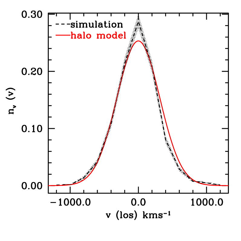
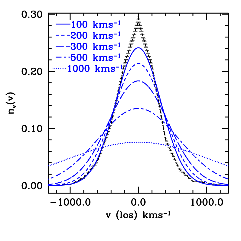
Figure 1 shows $n_{v}$ in the redshift slice between $z=0$ and $z=0.2$ both from the simulation and using Eq. (10) for the velocity probability distribution function. The analytical model agrees fairly well with the simulation; the error bars denote the $1\sigma$ errors including Poisson error and errors due to cosmic variance. Error modeling is discussed in detail in the next Section. Note that the error bars shown in Figure 1 are for a large future 5000 square degree velocity survey (one octant of the sky). Figures 2 and 3 compare the simulation with Eq. (11) for the mean pairwise streaming velocity (using the estimator Eq. (15)) and Eq. (20) for the velocity correlation function, respectively. The plots shows that the halo model agrees well with the simulated data at separations greater than 30 Mpc/h for velocity correlation, and greater than 40 Mpc/h for mean pairwise streaming velocity with a discrepancy somewhat larger than $1\sigma$ for $r$ between 30 and 40 Mpc/h. For the velocity probability distribution function, we find a good fit when the velocity data is smoothed over a scale of 10 Mpc. The smoothing on this scale reduces the effect of nonlinear physics which is difficult to model semianalytically.

Figure 2: A comparison between the mean pairwise streaming velocity $v_{ij}(r)$ evaluated directly using the Virgo lightcone numerical simulation (dashed line with 1$\sigma$ errors given by the blue dotted lines) and approximated using the analytic halo model formula, Eq. (11) (red solid curve). The error range includes Poisson and cosmic variance errors for one octant sky coverage, plus random measurement errors of 100 km/s.

Figure 3: Same as Figure 2 except for the velocity correlation $\langle v_{i}v_{j}\rangle_{\perp}(r)$ and the analytic formula Eq. (20).

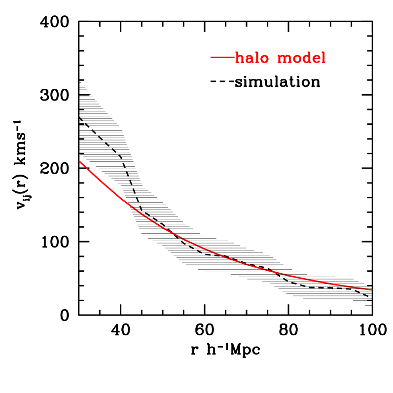
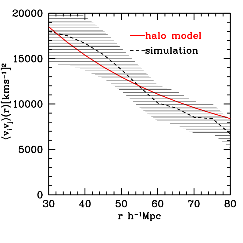
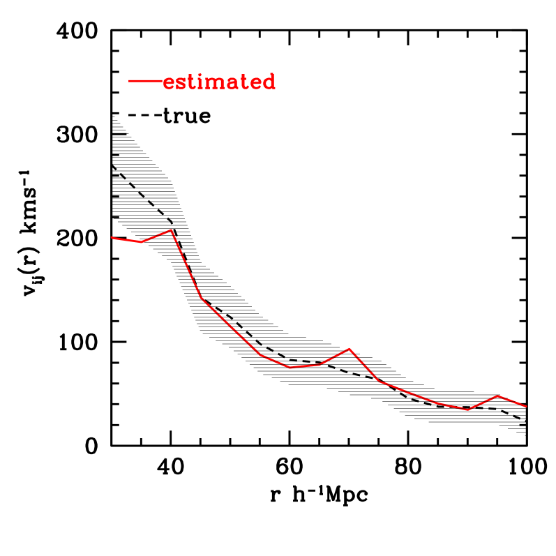
Figure 4 displays a comparison between the estimated mean pairwise streaming velocity $v_{ij}^{\rm est}$ obtained only from the radial component of velocity using Eq. (15) and the full $v_{ij}$ obtained from all three components of velocity in the simulation. For an ideal estimator, these quantities would be exactly the same; the actual estimator in general does quite well, except for a $1\sigma$ discrepancy at separations below 30 Mpc/h. The error range is the same as for Figure 2.

Figure 4: The solid red line shows $v_{ij}^{\rm est}$ computed from the Virgo simulation using only the radial velocities, Eq. (15), while the dashed line shows $v_{ij}$ and shaded 1$\sigma$ errors computed using all three velocity components, the same as in Fig. 2

.

IV Error Sources

Measurement of the radial velocity of individual clusters via their kinematic Sunyaev-Zeldovich signal is affected by various error sources, including detector noise in the microwave maps, separating the small signal from other larger signals at the same frequencies (particularly the thermal SZ signal, infrared point sources, and gravitational lensing by the cluster), the internal velocity dispersion of the intracluster medium, and X-ray temperature measurement errors. In this Section, we call the total error from all of these sources “measurement error.” We also consider separately the errors arising from cosmic variance and Poisson noise; both of these error sources are independent of the measurement errors for any individual cluster.

IV.1 Velocity Measurement Errors

Upcoming multi-frequency Sunyaev-Zeldovich measurements with arcminute resolution and few $\mu$K sensitivity have the potential to obtain galaxy cluster peculiar velocities. However, the kinematic Sunyaev-Zeldovich signal is small compared to the thermal SZ signal, and is spectrally indistinguishable from the primary microwave blackbody fluctuations or their gravitational lensing. In addition, radio and infrared galaxies contribute substantial signal in the microwave bands, and are expected to be spatially correlated with galaxy cluster positions Coble et al. (2007). Comparatively modest error sources can substantially hinder cluster velocity measurements if they are not well understood and accounted for.

Major potential sources of error in measuring the velocities of individual galaxy clusters include internal cluster gas velocities, the confusion-limited noise from point sources, uncertainties in extrapolating measured point sources to the frequencies of a particular experiment, instrumental noise, and the particular frequency bands available. Previous studies shows that primary microwave background fluctuations plus point sources set a confusion limited velocity error of around 200 km/s for an experiment with arcminute resolution and few $\mu$K sensitivity (Knox et al., 2004; Aghanim et al., 2001; Haehnelt and Tegmark, 1996), provided no other point source follow-up observations are utilized. The bulk flow of the gas in the intracluster medium contributes to an irreducible error of 100 to 150 km/s (Nagai et al., 2003; Diaferio et al., 2005a). Also, Ref. (Sehgal et al., 2005) shows that to extract velocity from SZ observations at the three ACT frequency channels (145, 220, and 280 GHz), a followup measurement of X-ray temperature of the cluster is needed to break a spectrum degeneracy between cluster gas velocity, optical depth, and temperature. While Ref. Diaferio et al. (2005a) studied over 100 simulated clusters, the rest of these studies use only a few. All of these error sources require detailed simulations of particular experiments observing realistic simulated clusters and optimal algorithms for extracting cluster velocities from measurements in particular frequency bands and at given instrumental noise levels. The ultimate distribution of velocity errors is still uncertain and future study in this direction is needed. In order to study the effect of measurement errors on parameter estimation, we make the simple assumption that velocity errors have a normal distribution with a magnitude between 100 and 500 km/s. Directly adding all of the known sources of error from previous studies gives velocity measurement errors typically in the range of 400 to 500 km/s; however, with further understanding of systematic errors and point sources, the error budget may be reduced.

IV.2 Redshift Errors

In addition to cluster velocity, we must measure cluster redshift to construct the estimators of the mean pairwise velocity and the velocity correlation, which involve knowledge of the separation vector between the two clusters. For clusters at cosmological distances, the Hubble contribution to its redshift will typically be much larger than its peculiar velocity contribution, which we can also correct for with a direct velocity measurement, so direct error in the cluster redshift will be the largest contributor to the cluster position error. Typically, we will be concerned with cluster separations larger than 30 Mpc/h, for which the cluster velocity field is in the mildly nonlinear regime and can be well described by the halo model approximation.

A redshift error of 500 km/sec corresponds to a direct Hubble distance error of around 5 Mpc/h, typically only 25% of the closest cluster separation of interest; even for redshift errors of 1000 km/sec, most pair separations will not be dominated by this error. For the remainder of this paper, we assume that the cluster sample for which velocities are determined also have spectroscopic redshifts from which their distances are determined, and we assume that the distance error effect on the cosmological parameters will be negligible compared to the direct velocity errors. For spectroscopic measurements of many galaxy clusters, the distance to lowest order is simply determined by the average of the galaxy redshifts, with an error given roughly by the cluster galaxy velocity dispersion divided by the square root of the number of clusters’ galaxies. Cluster line-of-sight velocity dispersions will typically be 500 km/sec, so multi-object spectroscopy can clearly provide adequate redshift measurements. The systematic error induced because not all clusters will be virialized is potentially important, although beyond the scope of this paper.

Spectroscopic redshifts for a galaxy cluster at $z=1$ requires roughly an hour of observation on an 8-m class telescope. Spectroscopic follow-up of hundreds of clusters per year is a large program for a single telescope; spectroscopic redshifts for thousands of clusters will comprise a multi-year program on more than one telescope. This is likely to be a significant portion of the effort and expense in building a cluster peculiar velocity survey with thousands of clusters. Note that cluster galaxy spectroscopic redshifts are also valuable for dynamical mass estimates; see, e.g., Diaferio et al. (2005b); Rines et al. (2003). The ACT collaboration has plans for spectroscopic follow-up observations of SZ-detected clusters using the Southern African Large Telescope (SALT), a new 10-meter class instrument. If only photometric redshifts are available, typically giving a distance accuracy of one to two percent times $1+z$, cosmological constraints must be re-evaluated. In general, constraints will be less stringent, although it is not immediately clear whether the resulting distance errors will have an effect which is significant compared to the velocity errors. In our case, redshift errors propagate only into the geometric portions of the mean pairwise streaming velocity and velocity correlation estimators, but the velocity errors are unaffected. This issue will be addressed in detail elsewhere.

IV.3 Cosmic Variance and Poisson Noise

In addition to measurement errors for individual cluster velocities, cosmological quantities are also subject to errors from cosmic variance (any particular region observed may have different statistical properties from the average of the entire universe) and Poisson errors due to the finite size of the cluster velocity sample used to estimate the velocity statistics. Here we discuss these errors for each of the three velocity statistics. Detailed derivations of the expressions in the rest of this Section are given in the Appendices.

IV.3.1 Probability Density Function

Consider a cluster velocity survey with a measured redshift for each cluster. For the probability density function, we write cosmic covariance between two different velocity–redshift bins $[v,z]_{i}$ and $[v,z]_{j}$ as $C^{n_{v}}_{ij}$, which can be expressed as

$$C^{n_{v}}(ij)=\frac{3D_{a_{i}}D_{a_{j}}}{R_{\Omega}}n_{i}n_{j}\int dkk^{2}P(k)j_{1}(kR_{\Omega})$$ (23)

where

$$n_{v}(v,z)=\frac{\int dmmb(m,a){\bar{n}(m)}p(v|m,\delta,a)}{\int dmm{\bar{n}(m)}}$$ (24)

and $R_{\Omega}$ is the comoving length of the redshift bin within the sky survey region Hogg (1999).

For Poisson errors, let $N_{i}$ be the total number of clusters in bin $i$. We are interested in the error in $n_{i}=N_{i}/N_{z}$ with $N_{z}$ the total number of clusters in a particular redshift bin summed over all velocities; the measured $n_{i}$ corresponds to the theoretical quantity $n_{v}(v,z)$, Eq. (10), integrated over the velocity–redshift bin $[v,z]_{i}$. The expression for Poisson errors can be written as

$$\delta n_{i}=({\sqrt{n}_{i}}+n_{i})/{\sqrt{N}_{z}}$$ (25)

where the first term is from the error in $N_{i}$ and the second from the error in $N_{z}$.

Random velocity measurement errors will smear out the velocity PDF. We quantify the effect of measurement errors by convolving the PDF with a normal distribution of velocity errors,

$$n_{v}^{\rm obs}(v,\delta v,z)=\int_{\delta v}dv\int_{v_{l}}^{v}dv^{\prime}f(v^{\prime},z)\exp[-(v^{\prime}-v)^{2}/{2\sigma_{v}^{2}}]$$ (26)

where $\sigma_{v}$ is the dispersion of the normally distributed velocity errors and the integral is over the velocity bin. Then the expression for the total covariance can be written as

$$C^{n_{v}}_{t}(v_{i},z_{i};v_{j},z_{j})=C^{n_{v}}(ij)+(\delta n_{i})^{2}\delta_{ij}$$ (27)

Figure 5: The effect of measurement errors on the velocity probability distribution function: from top to bottom, velocity measurement errors of $\sigma_{v}=$100, 200, 300, 500, and 1000 km/s. Also shown are the probability distribution function evaluated directly using the Virgo lightcone numerical simulation (dotted curve with error bars) from Figure 1

The various curves in Fig. 5 show the effect of random velocity errors of different sizes, Eq. (26), while the top dotted curve with shaded error region gives the actual value for the probability distribution function from the VIRGO simulation with Poisson plus cosmic variance errors. Smearing the distribution by random velocity errors is largely degenerate with the effect of varying cosmological parameters. This means that the velocity probability distribution function as a probe of cosmology is limited by how well the measurement error can be understood from simulated measurements.

IV.3.2 Mean Pairwise Streaming Velocity

The mean pairwise streaming velocity statistic is binned in pair separation and redshift. The cosmic covariance between two bins $[r,z]_{p}$ and $[r,z]_{q}$ can be written as

$$C^{v_{ij}}(pq)=\frac{32\pi}{9V_{\Omega}}\frac{H(a_{p})a_{p}}{1+\xi^{\rm halo}(r_{p},a_{p})}\frac{H(a_{q})a_{q}}{1+\xi^{\rm halo}(r_{q},a_{q})}\left(\frac{d\ln D_{a}}{d\ln a}\right)_{a_{p}}\left(\frac{d\ln D_{a}}{d\ln a}\right)_{a_{q}}\int dkk^{2}|P(k)|^{2}j_{1}(kr_{p})j_{1}(kr_{q}).$$ (28)

We add in quadrature the Poisson error and measurement error for $n_{\rm pair}$ cluster pairs and write the total covariance as

$$C^{v_{ij}}(r_{p},z_{p};r_{q},z_{q})=C^{v_{ij}}_{\rm cosmic}(pq)+\left(\frac{v_{ij}^{2}}{n_{\rm pair}}+\frac{2\sigma_{v}^{2}}{n_{\rm pair}}\right)\delta_{pq}$$ (29)

Figure 6: Fractional errors $\delta v_{ij}/v_{ij}$ for a cluster velocity survey covering 5000 square degrees: the red square points represents the Poisson error; black triangles represents cosmic variance and the Blue lines represents measurement errors (from bottom to top $\sigma_{v}$=100, 200, 300, 500 and 1000 km/s). Note that all the errors scales as $\sqrt{f}_{sky}$ for other survey areas.

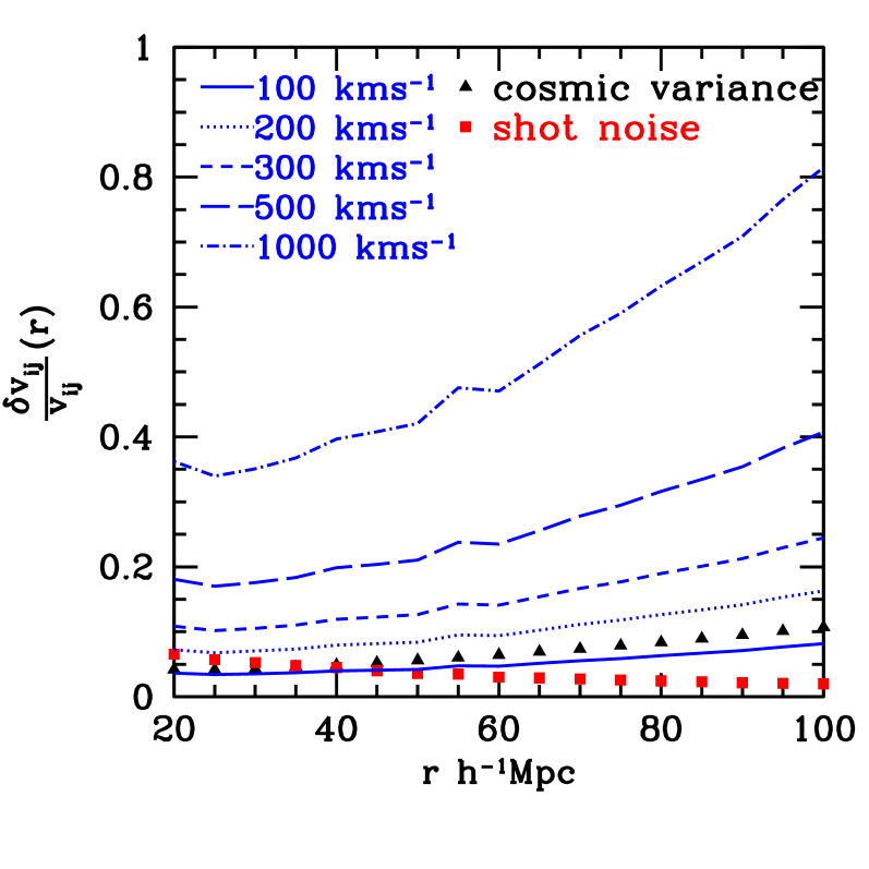
Figure 6 plots fractional errors for $v_{ij}$ as a function of pair separation for a survey area of 5000 deg². For a survey area $f_{\rm sky}$, fractional errors scales as roughly $\sqrt{f_{\rm sky}}$. Note that the Poisson error decreases for larger separation since more clusters pairs are available to average over, whereas cosmic variance has an increasing effect at larger separation. The combined effect of cosmic variance plus Poisson errors dominates the error budget when velocity measurement errors are below 200 km/s. Note that even when the measurement errors are as high as $\sigma_{v}=500$ km/s, the total error is typically 50% of the magnitude of mean pairwise streaming velocity. We will show in Sec. V that this fact makes mean pairwise streaming velocity a potentially useful probe to study cosmology.

IV.3.3 Velocity Correlation Function

Similarly for the velocity correlation function, the expression for cosmic covariance can be written as

$$C^{\langle v_{i}v_{j}\rangle}_{\rm cosmic}(pq) = \frac{8\pi}{V_{\Omega}{\bar{\rho}}^{2}(p){\bar{\rho}}^{2}(q)}\left[\frac{d\ln D_{a}}{d\ln a}\right]^{2}_{a_{p}}\left[\frac{d\ln D_{a}}{d\ln a}\right]^{2}_{a_{q}}\frac{a_{p}^{2}D^{2}_{a_{p}}H^{2}(a_{p})}{1+\xi^{\rm halo}(r_{p},a_{p})}\frac{a_{q}^{2}D^{2}_{a_{q}}H^{2}(a_{q})}{1+\xi^{\rm halo}(r_{q},a_{q})}$$ (30)

$$\qquad\qquad\qquad\qquad\times\int dkj_{1}(kr_{p})j_{1}(kr_{q})[P(k)]^{2}\langle p\rangle^{2}_{m}\langle q\rangle^{2}_{m}$$

using the notational abbreviation

$$\langle x\rangle_{m}\equiv\int dm\,m\frac{dn}{dm}W(kR(m))\frac{\sigma_{0}(m)}{\sigma_{-1}(m)}\,x.$$ (31)

In Eq. (30) we have ignored the contribution of the second ($I_{2}$) term in Eq. (20). At larger separations relevant here, this term, being weighted by $\xi(r)$, is an order of magnitude smaller than the first term and hence has negligible contribution to the cosmic variance.

Again we add in quadrature the Poisson error and measurement error for $n_{\rm pair}$ cluster pairs and write the total covariance as

$$C^{\langle v_{i}v_{j}\rangle}_{t}[r_{p},z_{p}|r_{q},z_{q}]=C^{\langle v_{i}v_{j}\rangle}(pq)+\left[\frac{\langle v_{i}v_{j}\rangle(r,z)}{\sqrt{n^{pair}(r,z)}}\right]^{2}+\left[\frac{1}{n^{pair}}\Sigma[\delta(v^{2})+(\delta v)^{2}]\right]^{2}$$ (32)

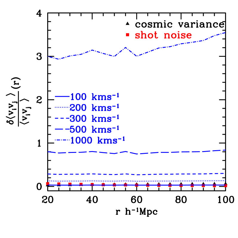
Figure 7 shows the various errors in the velocity correlation function. The trends are similar to those for mean pairwise streaming velocity. Measurement errors dominate the error budget for $\sigma_{v}>200$ km/s. Note however the increase in fractional errors with the increase in measurement errors. For $\sigma_{v}=500$ km/s, the contribution of measurement errors to the total error is almost 90%, nearly double that for the case of mean pairwise streaming velocity.

Figure 7: Same as in Figure 6 for the fractional error $\delta(\langle v_{i}v_{j}\rangle)/\langle v_{i}v_{j}\rangle$.

V Constraints on Dark Energy Parameters

Now we consider constraints on dark energy parameters for various survey areas and over a range of velocity errors. Following the Dark Energy Task Force, we describe the dark energy in terms of three phenomenological parameters: its current energy density $\Omega_{\Lambda}$, and two parameters $w_{0}$ and $w_{a}$ describing the redshift evolution of its equation of state $w(a)=w_{0}+(1-a)w_{a}$. Assuming a spatially flat universe, the set of cosmological parameters ${\bf p}$ on which the velocity field depends are the normalization of the matter power spectrum $\sigma_{8}$ (or equivalently the normalization constant $B$ in Eq. (5)), the power law index of the primordial power spectrum $n_{S}$, and the Hubble parameter $h$, plus the dark energy parameters. We perform a simple Fisher matrix analysis to find constraints on these parameters from measurements of the three velocity statistics described in Sec. II.

We consider a fiducial model similar to that assumed in the DETF report (Albrecht et al., 2006) with $\sigma_{8}=0.9$, $n_{S}=1$, $h=0.7$, $\Omega_{\Lambda}=0.72$, $w_{0}=-1$, $w_{a}=0$. To make quantitative comparisons with the conclusions of the DETF report, we compute values for the expression $[\sigma(w_{0})\sigma(w_{p})]^{-1}$, which is listed in the DETF summary tables. We refer to this as the “Figure of Merit” (FOM) for convenience, although this term refers to a slightly different quantity (inverse area of the ellipse of $95\%$ confidence limit in the $w_{p}-w_{a}$ plane) in the DETF report. Here $w_{p}$ is the equation of state at the pivot point defined as $w_{p}=w_{0}+(1-a_{p})w_{a}$ with $a_{p}=1+[F^{-1}]_{w_{0}w_{a}}/[F^{-1}]_{w_{a}w_{a}}$ and $F$ the Fisher information matrix for a given experiment.

Figure 8: The change in 1$\sigma$ parameter constraints with velocity error (normal distribution of width $\sigma_{v}$) for a 4000 deg² survey area, for the three statistics $n_{v}$ (blue dashed), $v_{ij}$ (red short dashed) and $\left\langle v_{i}v_{j}\right\rangle$ (black solid). The four panels are for the parameters $w_{0}$ (top left), $\Omega_{\Lambda}$ (top right), $w_{a}$ (bottom left), and the Figure of Merit (bottom right).

Table 1: 1$\sigma$ errors on dark energy parameters for a 4000 deg² survey area plus cosmological priors from Planck and HST (Albrecht et al., 2006; Freedman et al., 2001), assuming a spatially flat cosmology.

$\sigma_{v}$		$w_{0}$			$w_{a}$			$\Omega_{\Lambda}$			$[\sigma(w_{0})\sigma(w_{p})]^{-1}$
	${\langle v_{i}v_{j}\rangle}$	${v_{ij}}$	${n_{v}}$	${\langle v_{i}v_{j}\rangle}$	${v_{ij}}$	${n_{v}}$	${\langle v_{i}v_{j}\rangle}$	${v_{ij}}$	${n_{v}}$	${\langle v_{i}v_{j}\rangle}$	${v_{ij}}$	${n_{v}}$
100	0.06	0.083	0.099	0.16	0.26	0.2	0.007	0.007	0.016	165	104	94
200	0.1	0.1	0.11	0.29	0.33	0.25	0.014	0.008	0.018	60	76	71
300	0.18	0.13	0.14	0.53	0.42	0.34	0.026	0.009	0.019	20	54	50
500	0.39	0.18	0.25	1.32	0.61	0.65	0.046	0.012	0.026	5	31.5	21
1000	1.28	0.31	0.9	4.7	1.11	3.0	0.060	0.018	0.048	0.5	14.5	3.0

Table 2: Same as Table 2, for a 2000 deg² survey area.

$\sigma_{v}$		$w_{0}$			$w_{a}$			$\Omega_{\Lambda}$			$[\sigma(w_{0})\sigma(w_{p})]^{-1}$
	${\langle v_{i}v_{j}\rangle}$	${v_{ij}}$	${n_{v}}$	${\langle v_{i}v_{j}\rangle}$	${v_{ij}}$	${n_{v}}$	${\langle v_{i}v_{j}\rangle}$	${v_{ij}}$	${n_{v}}$	${\langle v_{i}v_{j}\rangle}$	${v_{ij}}$	${n_{v}}$
100	0.08	0.12	0.12	0.26	0.41	0.28	0.011	0.010	0.018	80	53	59
200	0.13	0.14	0.15	0.43	0.51	0.35	0.011	0.011	0.020	31	39	47
300	0.25	0.18	0.19	0.77	0.63	0.47	0.035	0.013	0.022	11	29	32
500	0.52	0.25	0.33	1.83	0.89	0.9	0.052	0.016	0.032	3	18	13
1000	1.8	0.42	1.26	6.7	1.48	4.2	0.061	0.022	0.061	0.75	7.9	1.6

Table 3: Same as Table 1, for a 400 deg² survey area.

$\sigma_{v}$		$w_{0}$			$w_{a}$			$\Omega_{\Lambda}$			$[\sigma(w_{0})\sigma(w_{p})]^{-1}$
	${\langle v_{i}v_{j}\rangle}$	${v_{ij}}$	${n_{v}}$	${\langle v_{i}v_{j}\rangle}$	${v_{ij}}$	${n_{v}}$	${\langle v_{i}v_{j}\rangle}$	${v_{ij}}$	${n_{v}}$	${\langle v_{i}v_{j}\rangle}$	${v_{ij}}$	${n_{v}}$
100	0.13	0.20	0.2	0.45	0.72	0.51	0.019	0.015	0.023	30	22	29
200	0.24	0.25	0.24	0.76	0.92	0.64	0.034	0.017	0.026	11	16	21
300	0.41	0.31	0.31	1.39	1.15	0.85	0.048	0.020	0.031	4.0	11	14
500	0.92	0.6	0.53	3.4	1.66	1.53	0.058	0.024	0.044	1.4	0.7	5.2
1000	3.6	0.78	2.42	13.3	3.0	8.0	0.061	0.033	0.061	0.38	3.3	0.7

The Fisher information matrix for each of the three statistics is Bhattacharya and Kosowsky (2007)

$$F_{\alpha\beta}=\sum_{i,j}\frac{\partial\phi(i)}{\partial p_{\alpha}}[C^{\phi}_{t}(ij)]^{-1}\frac{\partial\phi(j)}{\partial p_{\beta}}$$ (33)

where $\phi$ stands for either $n_{v}$, $v_{ij}(r,z)$ or $\langle v_{i}v_{j}\rangle(r,z)$, $C^{\phi}(ij)$ is the total covariance matrix in each bin for the statistic $\phi$, Eqs. (27), (29), and (32), and the partial derivatives are evaluated for the fiducial values of the cosmological parameters. The values $i$ and $j$ index the bins $[r,z]_{i}$ and $[r,z]_{j}$ for the mean pairwise streaming velocity and velocity correlation function, while for $\phi=n_{v}$, $i$ and $j$ refer to $[v,z]_{i}$ and $[v,z]_{j}$. The inverse of the Fisher matrix has diagonal elements which are estimates for the variances of each cosmological parameter marginalized over the values of the other parameters, and the non-diagonal elements give the correlations between parameters.

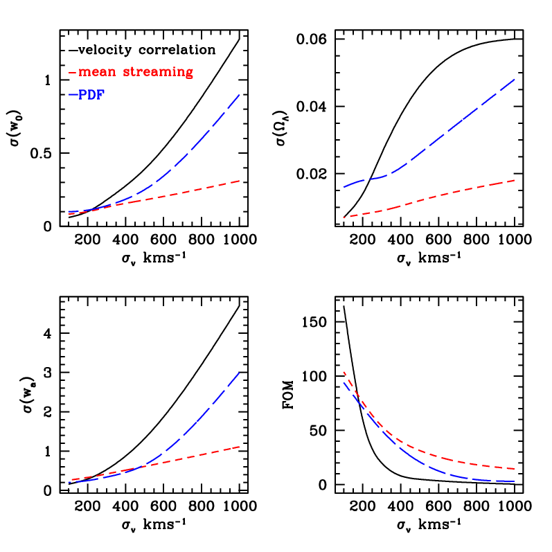
Figure 8 shows the degradation of parameter constraints with increasing velocity error $\sigma_{v}$ for a 4000 deg² survey area. It is evident that parameter constraints from $v_{ij}$ are more robust to increases in velocity error than those from $n_{v}$ and $\langle v_{i}v_{j}\rangle$. This is because $\delta v_{ij}$ depends linearly on $\sigma_{v}$, while $\delta\langle v_{i}v_{j}\rangle$ varies as $\sigma_{v}^{2}$ and for $n_{v}$ the distribution gets smeared with increases in $\sigma_{v}$. Constraints on $w_{0}$, $w_{a}$ and $\Omega_{\Lambda}$ change roughly by a factor of two and the constraint on the FOM by a factor of three, for the factor of five increase in $\sigma_{v}$ from 200 to 500 km/s. Compare this to the corresponding change for $\langle v_{i}v_{j}\rangle$: $w_{0}$, $w_{a}$ and $\Omega_{\Lambda}$ constraints change roughly by a factor of 6 to 8 and the FOM constraint by a factor of 30 for a similar change in $\sigma_{v}$. For $n_{v}$, the corresponding degradation in constraints are roughly by a factor 1.5 to 3 for $w_{0}$, $w_{a}$ and $\Omega_{\Lambda}$ while the FOM constraint degrades by roughly a factor of 4. Table 1 lists the constraints as a function of velocity error for a 4000 deg² survey area, while Tables 2 and 3 give constraints for 2000 deg² and 400 deg² respectively.

Note that the velocity correlation function $\langle v_{i}v_{j}\rangle$ provides the best constraints on the dark energy equation of state ($w_{0}$, $w_{a}$, and FOM) for $\sigma_{v}<200$ km/s. It might be possible to achieve such values of errors in future surveys with better understanding of point source contamination and other systematics. However for more realistic near-term errors of 500 km/s, the mean pairwise peculiar velocity $v_{ij}$ provides better constraints on dark energy parameters, and this statistic will be used in the following sections which consider how cosmological constraints will be improved by using cluster velocity information.

VI Complementarity of Cluster Velocities with Cluster Number Counts

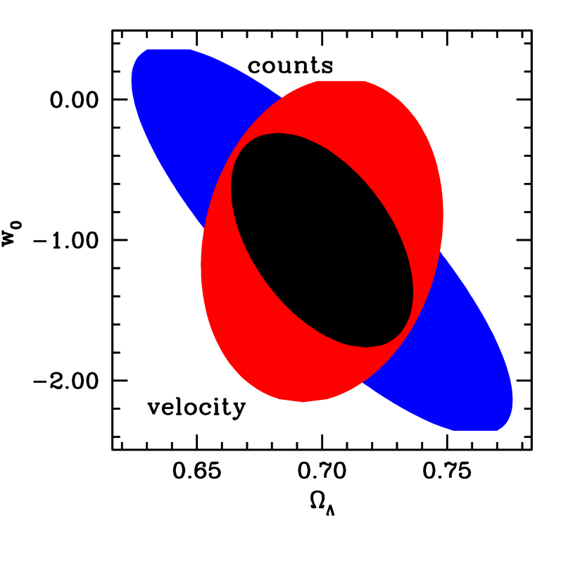
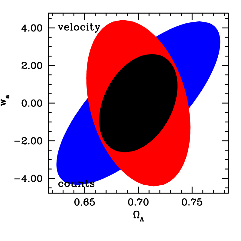
For a given SZ survey, we can potentially obtain both cluster counts and cluster peculiar velocities. Given these two different data sources from the same survey, what is the joint constraint on dark energy parameters they provide? Consider a fiducial Stage II survey of 4000 galaxy clusters proposed by the DETF report (Albrecht et al., 2006) (see Table 5 for details), plus the addition of cluster velocities with measurement error $\sigma_{v}=1000$ km/s, along with cosmic variance and Poisson errors to estimate the mean pairwise peculiar velocity statistic $v_{ij}$. This is not a particularly stringent velocity error, and it is likely obtainable with currently planned surveys with foreseeable follow-up observations or theoretical assumptions about cluster properties. Table 4 gives the constraint on the dark energy parameters derived considering cluster counts only, considering cluster velocities only, and the joint constraint from both. Also given are HST plus Planck prior constraints assuming a flat spatial geometry. We find cluster velocities provide a better constraint on $\Omega_{\Lambda}$ and $w_{0}$ than cluster counts, even for a measurement error of $\sigma_{v}=1000$ km/s. The constraint on $w_{a}$ is comparable for the two probes. The combined constraint is a factor of two better than the counts-only case for $\Omega_{\Lambda}$, $w_{0}$ and the Figure of Merit, and at least a 60% improvement for $w_{a}$. The relative complementarity between the two probes is shown in Figure 9.

We have assumed that the cluster velocity and cluster density observables are statistically uncorrelated. As they will likely be obtained from the same set of clusters, it is reasonable to ask whether this is actually true. A straightforward analytic calculation shows that the cross-correlation between velocity and density will be proportional to the matter bispectrum, so we expect it to be small compared to the signal from the velocity correlations, which are proportional to the matter power spectrum. We intend to confirm this prediction from sets of large-volume numerical simulations when these are available.

Figure 9: The relative complementarity of velocity and cluster counts. Shown are 1$\sigma$ error ellipses in the $w_{0}-\Omega_{\Lambda}$ plane (left) and the $w_{a}-\Omega_{\Lambda}$ plane (right) for 4000 clusters with normally-distributed velocity errors of $\sigma_{v}=1000km/s$. The three ellipses are for cluster velocities (red), cluster counts (blue) and the combination of both (black). Planck and HST cosmological priors (Albrecht et al., 2006; Freedman et al., 2001) and a spatially flat cosmology are assumed.

Table 4: 1$\sigma$ constraints for dark energy parameters for a fiducial cluster survey of 4000 clusters with velocity errors $\sigma_{v}=1000$ km/s, for cluster number counts, cluster velocities, and the two combined. Planck and HST cosmological priors (Albrecht et al., 2006; Freedman et al., 2001) plus spatially flat cosmology assumed.

Parameters	Priors	Counts	Velocity	Combined
$\Omega_{\Lambda}$[0.7]	0.062	0.052	0.033	0.025
$w_{0}$[-1]	$-$	0.94	0.78	0.52
$w_{a}$[0]	$-$	2.95	3.0	1.8
FOM	$-$	2.8	3.0	7.0

VII Comparison with DETF Proposed Experiments

The Dark Energy Task Force report (Albrecht et al., 2006) considers four different potential probes to study dark energy parameters: weak lensing(WL), baryon acoustic oscillations (BAO), cluster counts (CL) and SNIa (SN) luminosity distance measurements. The relative merits of these probes have been discussed in detail in the DETF report both for ongoing and future projects. In this section we compare our fiducial velocity survey with each of the four DETF probes. To assess the advantage of adding cluster mean pairwise peculiar velocity $v_{ij}$ as a dark energy probe, we have considered only the most optimistic forecasts for the DETF surveys (i.e. survey assumptions that provide maximum constraint to the FOM assuming a flat universe plus HST and Planck priors) for each Stage in the DETF report. Table 5 gives a brief description of the DETF surveys considered here and our corresponding assumed cluster velocity surveys. We have used the actual Fisher matrices used by the DETF team along with their priors for the following comparisons.

Table 5: Parameters defining various surveys discussed in the DETF report Albrecht et al. (2006), plus various cluster velocity surveys discussed here.

Stages	VEL	WL	SNIa	Cl	BAO
II	$N_{cl}=4000$, $f_{\rm sky}=0.01$	$f_{\rm sky}=0.0042$	SNLS	$N_{cl}=4000$	None
	$M_{min}>2\times 10^{14}M_{\odot}/h$		700 SNIa	$f_{\rm sky}=0.005$
	z=0.1-1.4		z=0.1-1.0
III	$N_{cl}=15000$	DES	2000 SNIa	$N_{cl}=30000$	$f_{\rm sky}=0.1$
	$f_{\rm sky}=0.05$	$f_{\rm sky}=0.1$	Spectroscopy
IV	$N_{cl}=30000$	SKA-o	Space	$N_{cl}=30000$	SKA-o
	$f_{\rm sky}=0.1$	$f_{\rm sky}=0.5$	2000 SNIa	$f_{\rm sky}=0.5$	$f_{\rm sky}=0.5$
		$z=0.1$–1.7		$z=0$–1.5

For the fiducial cluster velocity surveys, we have assumed that SZ surveys will be sensitive enough to detect the kSZ signal from all clusters with $M>2\times 10^{14}M_{\odot}/h$. To be consistent with the DETF report, the total number of clusters for each survey corresponds to $\sigma_{8}=0.9$. If $\sigma_{8}=0.76$ (Spergel et al., 2007) is used, then the corresponding number of clusters decreases by a factor of 30%. However, a velocity survey is sensitive to only the number of detected clusters and not the volume of the survey. So our conclusions will still be valid if the survey area is increased to compensate for a lower value of $\sigma_{8}$.

Figure 10: A comparison of the error in the dark energy density $\delta\Omega_{\Lambda}$ and the dark energy figure of merit obtained from velocity statistics with that from DETF probes. The top two panels are for Stage II experiments; the dark region shows the range in the parameter error for the DETF- assumed ranges in the measurement errors. For cluster velocities we assume a range from $\sigma_{v}=200$ to 1000 km/sec. The middle panels show the results for Stage IV measurements. The bottom panels show the relative improvement in parameter measurements at Stage IV when cluster velocities are combined with all of the other DETF probes.

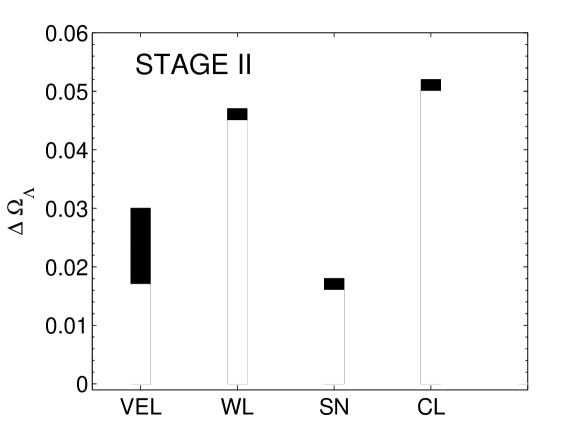
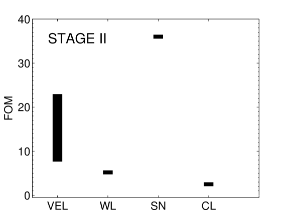
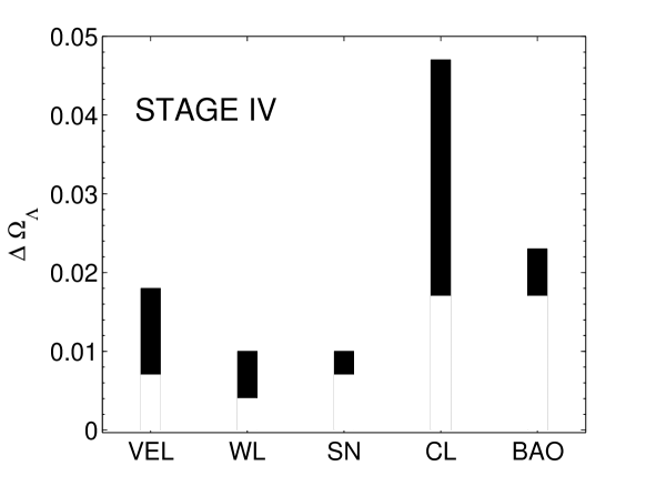
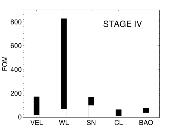
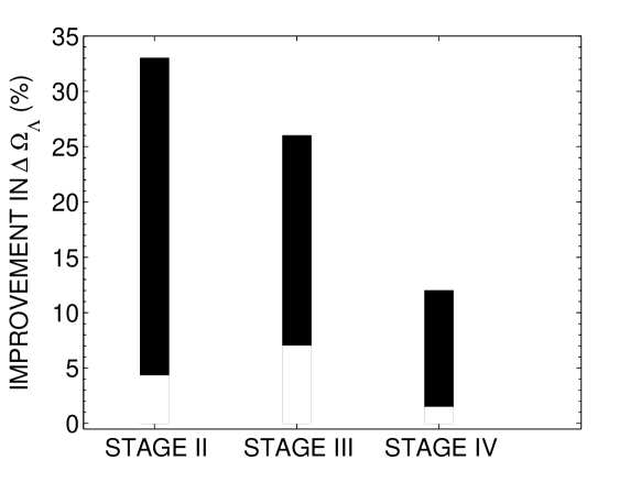
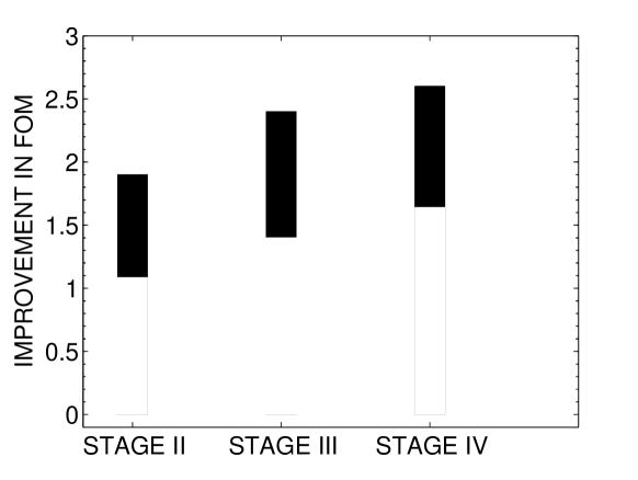
A comparison of velocity with other probes is shown in Figure 10. HST and Planck cosmological priors and spatially flat cosmology are assumed for all the probes. Each plot shows a range of parameter errors for each experiment, corresponding to cluster velocity measurement errors ranging between 200 and 1000 km/sec, and other measurement errors as in the DETF report. At Stage II, velocity provides a competitive constraint on $\Omega_{\Lambda}$ compared to SNIa, and much better constraints than weak lensing or cluster number counts. Even a modest velocity survey would yield a factor of two better constrain on $\Omega_{\Lambda}$ than cluster counts or weak lensing. Cluster velocities also provide two to three times better constraints to the figure of merit compared to weak lensing or cluster counts at Stage II. Ultimately at Stage IV, however, weak lensing provides the most accurate measurements of dark energy density and the figure of merit. But constraints from velocity are competitive with those from supernovae and better than those from cluster counts or baryon acoustic oscillations. Stage II and III experiments yield an average 20% improvement in cosmological parameter determination, and Stage IV about a 7% improvement, when velocity information is combined with the rest of the dark energy experiment results. This corresponds to an improvement by factors of 1.5 to 2.5 in the dark energy figure of merit. These types of statistical comparisons of course assume zero systematic errors; cluster velocities will ultimately be more valuable than these numbers indicate, due to their completely different systematic errors from the other challenging techniques. All of these methods will in the end be dominated by systematic, not statistical, errors.

VIII Discussion

The various studies of galaxy cluster peculiar velocities in this paper yield a number of interesting conclusions. The measurement of peculiar velocities of objects at cosmological distances is of fundamental importance, as it directly probes the evolution of the gravitational potential. The kinematic Sunyaev-Zeldovich effect in clusters of galaxies promises a direct tracer of this signal, with errors largely independent of cluster redshift. Although the current uncertainty in velocity measurements is large with $\sigma_{v}\approx 1000$ km/s (Benson et al., 2003) for individual clusters, upcoming multi-band experiments like ACT (Kosowsky, 2003) or SPT (Ruhl et al., 2004) with arcminute resolution and few $\mu$K sensitivity have the potential to measure peculiar velocities with velocity errors of a few hundred km/s for large samples of clusters, opening a new window on the evolution of the universe. We have considered three separate cluster velocity statistics here, computing them using the halo model and comparing with numerical results. For surveys with thousands of cluster velocities with errors of a few hundred km/sec, dark energy constraints competitive with other major techniques (cluster number counts, baryon acoustic oscillations, supernova redshift- distance measurements, and weak lensing) can be obtained from the mean pairwise peculiar velocity $v_{ij}$, with different systematic errors. Even for velocity errors as large as 1000 km/s for individual clusters, a velocity catalog for several thousand clusters can improve dark energy constraints from the corresponding cluster number counts by a factor of two.

Throughout this work, we have simply assumed that cluster velocities can be extracted with normal errors and no bias from a Sunyaev-Zeldovich sky survey of sufficient angular resolution and low enough noise. Connecting the measured SZ signal to the cluster velocity is a non-trivial task. The three ACT measured frequencies at 145, 220, and 270 GHz have a degeneracy which prevents the cluster velocity from being determined uniquely along with the cluster optical depth and temperature Sehgal et al. (2005); Holder (2004). This can be remedied several ways, including adding other microwave bands Holder (2004) or X-ray temperature measurements Sehgal et al. (2005), or assuming cluster scaling relations between various measurable quantities Verde et al. (2002); McCarthy et al. (2003).

Further complications arise because the measured signal is not due only to the Sunyaev-Zeldovich distortions, but also contains the blackbody primordial microwave fluctuations, gravitational lensing of the microwave background, infrared and radio point sources which can be correlated with galaxy cluster positions, and galactic dust (see Sehgal et al. (2007) for a description of sky simulations incorporating all of these signals). The kinematic SZ signal must be separated from all of the others via a combination of frequency and spatial filtering. With sufficient data, this can clearly be done uniquely, but with limited wave bands, spatial resolution, and noise levels, any kSZ signal extraction will be subject to some amount of measurement error. Evaluation of this error for various observing strategies is important and we are currently pursuing it using simulations. Even with perfect separation, internal cluster gas motions provide an irredicible error floor for kSZ cluster velocity measurements of around 100 km/sec Nagai et al. (2003); Diaferio et al. (2005a).

Component separation and other issues may also lead to systematic errors. We are currently modeling systematic errors in velocity measurements in some detail, but it is clear that at minimum, cosmological constraints based on cluster velocity measurements are much less prone to systematic errors due to uncertainties in the relation between SZ distortion and cluster mass than constraints based on cluster number counts Francis et al. (2005); Lima and Hu (2005). This is potentially the dominant systematic error for cluster number count studies, and largely mitigating it is one strong incentive for pursuing cluster velocities as an alternative probe of dark energy. An additional advantage of using cluster velocities is that the cluster velocity distribution function $n_{v}$ should be symmetric with respect to positive and negative peculiar velocities, by homogeneity of the universe. Departures from symmetry are easily diagnosed and can be used as a monitor of unknown systematic errors. The downside of cluster velocities is that the kSZ signal is much smaller than the thermal SZ signal, on the order of 5 to 10 $\mu$K for large clusters with typical peculiar velocities. Separating this small signal from other larger ones may lead to different systematic errors. But potential constraints on dark energy from cluster velocities are good enough, and the other methods of measuring dark energy properties are hard enough, that building a cluster velocity catalog with a different set of systematic errors from other techniques is surely valuable.

A number of further lines of work related to cluster velocities are worth pursuing. Here we have considered three different galaxy cluster velocity statistics: the velocity probability distribution function $n_{v}$, the mean pairwise velocity dispersion $v_{ij}$, and the velocity correlation function $\langle v_{i}v_{j}\rangle$. Each constrains well a different set of cosmological quantities. We have not attempted a joint analysis, finding the combined cosmological constraints from all three statistics: the correlations between the statistics are complicated, and no clear way to derive them analytically presents itself. Proper joint constraints will require numerical evaluation of the correlations between statistics from sets of large cosmological simulations, which is feasible but demanding. A related question is the extent to which these three statistics, which are convenient from a theoretical and observational point of view, exhaust the useful cosmological information on dark energy constraints: are there other velocity statistics which, when combined with these three using the correct correlations, would further tighten the constraints? This is an open, and challenging, question.

On the numerical front, we have performed limited tests comparing the VIRGO simulation results with the halo-model expressions for the velocity statistics here, finding reasonable agreement for the particular cosmological model the simulation is based on. This is encouraging, but it would be reassuring to have explicit comparisons between theory and simulation for a wider range of models. Such computations require cosmological simulations over very large volumes, to capture a sufficient number of clusters with large enough masses, but can be done with fairly low mass resolution, since we only care about bulk cluster properties and not internal cluster details. Sets of such simulations are currently in progress.

The kinematic SZ signal does not directly measure cluster peculiar velocity, but rather is proportional to a line-of-sight integral of the cluster gas’ local peculiar velocity times its local density. Thus the kSZ effect is actually proportional to the cluster gas momentum with respect to the cosmic rest frame. We can sidestep the entire difficult observational issue of inferring cluster velocities from kSZ measurements by using cluster momenta instead. We then need theoretical calculations for the cluster momentum statistics corresponding to the velocity statistics considered here. Momentum statistics have the possibility of being just as cosmologically constraining, but easier to compare with observations. We have not found any suitable analytic approximations to the cluster momentum statistics, but this could also be evaluated numerically using large-volume, low- resolution N-body simulations mentioned above. The other related issue is connecting the cluster mass, which is used to evaluate cluster momenta in an N-body simulation, to the cluster gas mass, which gives the SZ signal. We need to understand the extent to which the cluster gas fraction is constant, or the extent to which we can understand its statistical distribution. We have already made initial steps to investigate this issue, finding, among other things, that the gas fraction in galaxy groups is affected non-negligably by quasar feedback, which heats the gas and suppresses star formation. However, at mass scales substantially below galaxy clusters, the gas fraction appears to be reasonably independent of mass. Probing this relation for clusters is a challenging computational issue, requiring sophisticated hydrodynamical simulations in much larger volumes to obtain information about galaxy clusters large enough to be of SZ interest.

As with so many cosmological sources of information, the advent of the dark energy era has given a new urgency to precision measurements. Galaxy cluster velocities, obtained via their kinematic Sunyaev-Zeldovich signal, directly probe the growth of structure in the universe via gravitational instability. The signals are small, but the advantages manifest. We firmly advocate that cluster velocities should be added to the arsenal of tactics now trained on the dark energy issue.

Appendix A Errors for the Probability Density Function

A.1 Poisson Error

Let $N_{z}$ be the number of halos in redshift bin $z+\delta z$, and $N_{v}$ be the number of halos in both the redshift bin $z+\delta z$ and the velocity bin $v+\delta v$. In a given velocity bin, the fractional density The observable in the normalized histogram of cluster velocities in a given redshift bin is then $n_{v}=N_{v}/N_{z}$. Thus $n_{v}$ suffers from uncertainties in both numerator and denominator. We write the uncertainty in $n_{v}$ as

$$\frac{\delta n_{v}}{n_{v}}=\frac{\delta N_{v}}{N_{v}}+\frac{\delta N_{z}}{N_{z}}$$

Assuming Poisson errors, $\delta N_{v}=\sqrt{N_{v}}$ and $\delta N_{z}=\sqrt{N_{z}}$. We write

$$\delta n_{v}={\sqrt{n}_{v}}/{\sqrt{N}_{z}}+n_{v}/{\sqrt{N}_{z}}=\frac{{\sqrt{n}_{v}}[1+{\sqrt{n}_{v}}]}{{\sqrt{N}_{z}}}$$ (34)

A.2 Cosmic Variance Error

Write the cosmic covariance between two different bins $[v_{i},z_{i}]$ and $[v_{j},z_{j}]$ as $C^{n_{v}}_{ij}$; here $v_{i}$ denotes a particular velocity bin at an epoch of redshift $z_{i}$. $C^{n_{v}}_{ij}$ is defined as

$$C^{n_{v}}(ij)=\left<(\hat{n}_{vi}-n_{vi})(\hat{n}_{vj}-n_{vj})\right>$$ (35)

where $\hat{n}_{v}$ denotes the estimated PDF and $n_{vi}=n_{v}(v_{i},z_{i})$ etc. Using $n(m,\delta,{\bf x})=(1+b(m)\delta({\bf x}))\bar{n}(m)$ and $\hat{n}_{v}=V(r)^{-1}[\int d^{3}{\bf x}\int dm\,mn(m|\bar{\delta},{\bf x})p(v\,|\,m,\delta)]/\int dm\,mn(m|\delta)$,

$$C^{n_{v}}(ij)=b(m_{i},z_{i})b(m_{j},z_{j})f_{i}f_{j}\left<\delta({\bf x}_{i},z_{i})\delta^{*}({\bf x}_{j},z_{j})\right>$$ (36)

where $\langle...\rangle$ denotes the ensemble average over the survey volume $V_{\Omega}$ and can be written as

$$\left<\delta_{i}\delta_{j}\right>=\frac{1}{V_{\Omega}}\int_{V_{\Omega}}d^{3}{\bf r}\int\int d^{3}{\bf x}d^{3}{\bf x^{\prime}}W({x})W({x^{\prime}})\delta({\bf x},a)\delta({\bf x^{\prime}},a^{\prime})\delta^{3}_{D}({\bf x}-{\bf x^{\prime}}-{\bf r})$$ (37)

where

$$\delta({\bf x},a)\equiv D_{a}\delta({\bf x})=D_{a}\int d^{3}{\bf k}\,\delta({\bf k})e^{i{\bf k}\cdot{\bf x}},$$ (38)

$W(x)$ is the tophat window function defined after Eq. (1) and $\delta({\bf x})$ is the field describing linear comoving density perturbations evolved to the present; the three-dimensional Dirac delta distribution is written as $\delta^{3}_{D}({\bf x})$. We can then write

$$\left<\delta_{i}\delta_{j}\right> = \frac{D_{a_{i}}D_{a_{j}}}{V_{\Omega}}\int_{V_{\Omega}}d^{3}{\bf r}\int\int d^{3}{\bf x}d^{3}{\bf x^{\prime}}W(x)W(x^{\prime})\delta({\bf x})\delta({\bf x^{\prime}})\delta^{3}_{D}({\bf x}-{\bf x^{\prime}}-{\bf r})$$ (39)

$$= \frac{D_{a_{i}}D_{a_{j}}}{V_{\Omega}}\int d^{3}{\bf r}\int\int d^{3}{\bf k}d^{3}{\bf k^{\prime}}\delta(\bf k)\delta^{*}(\bf k^{\prime})e^{-i{\bf k}\cdot{\bf r}}h({\bf k}-{\bf k^{\prime}},{\bf r}).$$

where we write conventionally Eisenstein and Zaldarriaga (2001)

$$h({\bf k},{\bf r})\equiv\frac{1}{V(r)}\int d^{3}{\bf x}W(x)W(|{\bf x}+{\bf r}|)e^{i{\bf k}\cdot{\bf x}}.$$ (40)

In the limit of a survey region large compared to the scale $r$, $h({\bf k},{\bf r})\sim\delta^{3}_{D}({\bf k})$, $r\ll R_{\Omega}$ (Takada and Bridle, 2007; Eisenstein and Zaldarriaga, 2001) with the convenient notation $V_{\Omega}=4\pi R_{\Omega}^{3}/3$ for a spherical survey volume, giving

$$\int d^{3}{\bf x}W(x)W(|{\bf x}+{\bf r}|)e^{i({\bf k}-{\bf k^{\prime}})\cdot{\bf x}}{\int d^{3}{\bf x}W^{2}(x)}\propto\delta^{3}_{D}({\bf k}-{\bf k^{\prime}}).$$ (41)

Then

$$\left<\delta_{i}\delta_{j}\right>=\frac{4\pi R_{\Omega}^{2}D_{ai}D_{aj}}{V_{\Omega}}\int dkk^{2}P(k)j_{1}(kR_{\Omega}),$$ (42)

so $C^{n_{v}}(ij)$ can be written as

$$C^{n_{v}}(ij)=\frac{3D_{a_{i}}D_{a_{j}}}{R_{\Omega}}n_{i}n_{j}\int dkk^{2}P(k)j_{1}(kR_{\Omega})$$ (43)

where

$$n_{v}(v,z)=\frac{\int dmmb(m,a){\bar{n}(m)}p(v|m,\delta,a)}{\int dmm{\bar{n}(m)}}$$ (44)

which is equivalent to Eq. (23). The expression $p(v|m,\delta)$ is defined in Eq. (6).

Appendix B Errors for the Mean Pairwise Streaming Velocity

B.1 Poisson Error and Measurement Error

We begin with Eq. (15) for the estimator of the mean pairwise streaming velocity. Assume a particular velocity is measured with an accuracy $\delta v$. So the error $\delta v_{ij}$ in $v_{ij}$ can be written as

$$\frac{\delta v_{ij}}{v_{ij}}=\frac{\delta\Sigma_{ij}[v_{i}-v_{j}]}{\Sigma_{ij}[v_{i}-v_{j}]}+\frac{\delta n_{p}}{n_{p}},$$ (45)

so that

$$\delta v_{ij}=\frac{\sqrt{2}\left[\Sigma_{i}\delta v^{2}_{i}\right]^{1/2}}{n_{p}}+\frac{v_{ij}}{\sqrt{n}_{p}}=\frac{1}{\sqrt{n}_{p}}\left(\sqrt{2}\sigma_{v}+v_{ij}\right)$$ (46)

where we have used $\delta n_{p}=\sqrt{n}_{p}$ assuming a Poisson distribution, and

$$\delta\Sigma_{ij}\left[v_{i}-v_{j}\right]=\sqrt{2}[\delta v^{2}_{1}+\delta v^{2}_{2}+...+\delta v^{2}_{n_{p}}]^{1/2}=\sqrt{2}{\sqrt{n}_{p}}\sigma_{v}.$$ (47)

Here the individual velocity errors are added in quadrature and the last line follows from the central limit theorem.

B.2 Cosmic Variance Error

The cosmic covariance for mean pairwise streaming velocity between two separation and redshift bins $[r_{p},z_{p}]$ and $[r_{q},z_{q}]$ can be written as

$$C^{v_{ij}}(pq) = \left<\left(v_{ij}(p)-{\hat{v}_{ij}(p)}\right)\left(v_{ij}(q)-{\hat{v}_{ij}(q)}\right)\right>=\left<{\hat{v}_{ij}}(p){\hat{v}_{ij}}(q)\right>-v_{ij}(p)v_{ij}(q)$$ (48)

where ${\hat{v}_{ij}}$ is the estimated mean pairwise streaming velocity from the survey volume and $v_{ij}$ is its cosmic mean value, $\langle{\hat{v}_{ij}}\rangle=v_{ij}$. Using the expression for mean pairwise streaming velocity given in Eq. (11), the above expression can be written as

$$C^{v_{ij}}(pq) = \frac{1}{1+\xi^{\rm halo}(r_{p},a_{p})}\left[\frac{2}{3}r_{p}H(a_{p})a_{p}\left(\frac{d\ln D_{a}}{d\ln a}\right)_{a_{p}}\right]\frac{1}{1+\xi^{\rm halo}(r_{q},a_{q})}\left[\frac{2}{3}r_{q}H(a_{q})a_{q}\left(\frac{d\ln D_{a}}{d\ln a}\right)_{a_{q}}\right]$$ (49)

$$\qquad\qquad\qquad\qquad\times\left[\left<{\hat{\bar{\xi}}}(r_{p}){\hat{\bar{\xi}}}(r_{q})\right>-{\bar{\xi}}(r_{p}){\bar{\xi}}(r_{q})\right],$$

where $\hat{\bar{\xi}}$ is an estimator for the volume-averaged correlation function

$$\bar{\xi}(r)\equiv\frac{1}{V(r)}\int_{0}^{r}dr^{\prime}\,r^{\prime 2}\xi(r^{\prime}).$$ (50)

An estimator $\hat{\xi}(r)$ for the two-point correlation function $\xi(r)$ is

$$\hat{\xi}(r)=\frac{1}{V(r)}\int d^{3}{\bf x^{\prime}}W(x^{\prime})\int d^{3}{\bf x}W(x)\delta({\bf x})\delta({\bf x^{\prime}})\delta^{3}_{D}({\bf x}-{\bf x^{\prime}}-{\bf r}),$$ (51)

so an estimator for the volume-averaged correlation function can be written as

$${\hat{\bar{\xi}}}(r)=\frac{1}{V(r)}\int_{V(r)}d^{3}{\bf r^{\prime}}\frac{1}{V((r^{\prime})}\int d^{3}{\bf x}W(x)\int d^{3}{\bf x^{\prime}}W(x^{\prime})\delta({\bf x})\delta({\bf x^{\prime}})\delta^{3}_{D}({\bf x}-{\bf x^{\prime}}-{\bf r^{\prime}})$$ (52)

where the survey volume is given by $V(r)\equiv\int d^{3}{\bf x}\,W(x)W(|{\bf x}+{\bf r}|)$ for a normalized window function $\int d^{3}{\bf x}\,W(x)=1$. Fourier transforming $\delta(x)$, we can write

$${\hat{\bar{\xi}}}(r) = \frac{1}{V(r)}\int_{V(r)}d^{3}{\bf r^{\prime}}\frac{1}{V(r^{\prime})}\int d^{3}{\bf r^{\prime}}\int d^{3}{\bf x}W(x)\int d^{3}{\bf x^{\prime}}W(x^{\prime})\delta^{3}_{D}({\bf x}-{\bf x^{\prime}}-{\bf r^{\prime}})\int\int d^{3}{\bf k}d^{3}{\bf k^{\prime}}\delta({\bf k})\delta^{*}({\bf k^{\prime}})e^{i({\bf k}\cdot{\bf x}-{\bf k^{\prime}}\cdot{\bf x^{\prime}})}$$ (53)

$$= \frac{1}{V(r)}\int_{0}^{r}d^{3}{\bf r^{\prime}}\int\int d^{3}{\bf k}d^{3}{\bf k^{\prime}}\delta({\bf k})\delta^{*}({\bf k^{\prime}})e^{-i{\bf k}\cdot{\bf r^{\prime}}}h({\bf k}-{\bf k^{\prime}},{\bf r^{\prime}}).$$

Using $\langle\hat{\bar{\xi}}(r)\rangle={\bar{\xi}}(r)$, we can then write

$$C^{\bar{\xi}}(pq) = \left[\left<{\hat{\bar{\xi}}}(r_{p}){\hat{\bar{\xi}}}(r_{q})\right>-{\bar{\xi}}(r_{p}){\bar{\xi}}(r_{q})\right]$$ (54)

$$= \frac{1}{V(r_{p})V(r_{q})}\int_{0}^{r_{p}}d^{3}{\bf r}e^{-i{\bf k}\cdot{\bf r}}h({\bf k}-{\bf k^{\prime}},{\bf r})\int_{0}^{r_{q}}d^{3}{\bf r^{\prime}}e^{-i{\bf k}\cdot{\bf r^{\prime}}}h^{*}({\bf k}-{\bf k^{\prime}},{\bf r^{\prime}})$$

$$\times \int d^{3}{\bf k}\int d^{3}{\bf k^{\prime}}\int d^{3}{\bf k_{1}}\int d^{3}{\bf k^{\prime}_{1}}\left[\left<\delta({\bf k})\delta^{*}({\bf k^{\prime}})\delta({\bf k_{1}})\delta^{*}({\bf k^{\prime}_{1}})\right>-\left<\delta({\bf k})\delta^{*}({\bf k^{\prime}})\right>\left<\delta({\bf k_{1}})\delta^{*}({\bf k^{\prime}_{1}})\right>\right].$$

The term in brackets can be written as

$$[...]=\delta^{3}_{D}({\bf k}+{\bf k_{1}})P(k)\delta^{3}_{D}({\bf k^{\prime}}+{\bf k^{\prime}_{1}})P(k^{\prime})+\delta^{3}_{D}({\bf k}-{\bf k^{\prime}_{1}})P(k)\delta^{3}_{D}({\bf k^{\prime}}-{\bf k_{1}})P(k^{\prime}).$$ (55)

Substituting this expression into Eq. (54) gives

$$C^{\bar{\xi}}(pq)=\frac{1}{V(r_{p})V(r_{q})}\int d^{3}{\bf k}\int d^{3}{\bf k^{\prime}}P(k)P(k^{\prime})\left(e^{i{\bf k}\cdot({\bf r}-{\bf r^{\prime}})}+e^{-i{\bf k}\cdot{\bf r}-i{\bf k^{\prime}}\cdot{\bf r^{\prime}}}\right)\int_{0}^{r_{p}}d^{3}{\bf r}h({\bf k}-{\bf k^{\prime}},{\bf r})\int_{0}^{r_{q}}d^{3}{\bf r^{\prime}}h^{*}({\bf k}-{\bf k^{\prime}},{\bf r^{\prime}}).$$ (56)

As in the previous appendix, for large surveys such that $r<<R_{\Omega}=(3V_{\Omega}/4\pi)^{1/3}$, $h({\bf k}-{\bf k^{\prime}},{\bf r})\sim\delta^{3}_{D}({\bf k}-{\bf k^{\prime}})$ and (Takada and Bridle, 2007; Eisenstein and Zaldarriaga, 2001)

$$hh^{*}=\frac{\int d^{3}{\bf x}W^{2}(x)W(|{\bf x}+{\bf r}|)W(|{\bf x}+{\bf r^{\prime}}|)}{V(r_{p})V(r_{q})}\sim\frac{1}{V_{\Omega}}.$$ (57)

So Eq. (56) can be written as

$$C^{\bar{\xi}}(pq) = \frac{1}{V_{\Omega}V(r_{p})V(r_{q})}\int d^{3}{\bf k}|P(k)|^{2}\int_{0}^{r_{p}}\int_{0}^{r_{q}}d^{3}{\bf r}d^{3}{\bf r^{\prime}}\left(e^{i{\bf k}\cdot({\bf r}-{\bf r^{\prime}}}+e^{-i{\bf k}\cdot({\bf r}+{\bf r^{\prime}})}\right)$$ (58)

$$= \frac{8\pi}{V_{\Omega}r_{p}r_{q}}\int dkk^{2}|P(k)|^{2}j_{1}(kr_{p})j_{1}(kr_{q})$$

Substituting the above result in Eq (49), we obtain the final expression for cosmic covariance as

$$C^{v_{ij}}(pq)=\frac{32\pi}{9V_{\Omega}}\frac{H(a_{p})a_{p}}{1+\xi^{\rm halo}(r_{p},a_{p})}\frac{H(a_{q})a_{q}}{1+\xi^{\rm halo}(r_{q},a_{q})}\left(\frac{d\ln D_{a}}{d\ln a}\right)_{a_{p}}\left(\frac{d\ln D_{a}}{d\ln a}\right)_{a_{q}}\int dkk^{2}|P(k)|^{2}j_{1}(kr_{p})j_{1}(kr_{q}).$$ (59)

On scales of interest, $\xi^{\rm halo}\ll 1$, so Eq. (59) reduces to Eq. (28).

Appendix C Errors for the Velocity Correlation Function

C.1 Poisson Error and Measurement Error

The expression for the perpendicular velocity correlation $\langle v_{i}v_{j}\rangle_{\perp}(r)$ for a particular separation $r$ can be written as

$$\langle v_{i}v_{j}\rangle(r)=\frac{\Sigma_{ij}[v_{i}v_{j}]_{\perp}}{n_{p}}$$ (60)

where we abbreviate $[v_{i}v_{j}]_{\perp}\equiv([{\bf r_{i}}-{\bf r_{j}}]\times{\bf v}_{i})\cdot([{\bf r_{i}}-{\bf r_{j}}]\times{\bf v}_{j})$ the product of the velocity components perpendicular to the direction connecting the two positions. As before, ${\bf v}_{i}$ is the velocity of halo $i$, which is measured with a normal error in its magnitude of $\delta v$, and $n_{p}$ is the number of pairs in the survey volume for a given separation distance $r$. For the rest of the appendix, we drop the perpendicular subscript for convenience. So the measurement error in $\langle v_{i}v_{j}\rangle$ can be written as

$$\langle v_{i}v_{j}\rangle+\delta\langle v_{i}v_{j}\rangle = \frac{1}{n_{p}}\Sigma_{ij}[v_{i}v_{j}+2v_{j}\delta v_{i}+\delta v_{i}\delta v_{j}]$$

$$\delta\langle v_{i}v_{j}\rangle = \frac{1}{n_{p}}\Sigma_{ij}[2v_{j}\delta v_{i}+\delta v_{i}\delta v_{j}]$$ (61)

$$= \frac{1}{n_{p}}\Sigma[\delta(v^{2})+(\delta v)^{2}]$$

Similarly, the Poisson error is $\langle v_{i}v_{j}\rangle[\delta n_{p}/n_{p}]=\langle v_{i}v_{j}\rangle/{\sqrt{n}_{p}}$.

C.2 Cosmic Variance Error

The cosmic covariance for the velocity correlation function between two bins $[r_{p},z_{p}]$ and $[r_{q},z_{q}]$, one of separation $r_{p}$ at epoch $z_{p}$ and the other of separation $r_{q}$ at redshift $z_{q}$, can be written as

$$C^{\langle v_{i}v_{j}\rangle}(pq) = \left<\left(\left<v_{i}v_{j}\right>(p)-\left<{\langle\widehat{v_{i}v_{j}}\rangle}\right>(p)\right)\left(\left<v_{i}v_{j}\right>(q)-\left<{\widehat{v_{i}v_{j}}}\right>(q)\right)\right>$$ (62)

$$= \left<\widehat{v_{i}v_{j}}\right>(p)\left<\widehat{v_{i}v_{j}}\right>(q)-\left<v_{i}v_{j}\right>(p)\left<v_{i}v_{j}\right>(q)$$

As in the case of $v_{ij}(r)$, we first derive an estimator for $v_{i}v_{j}(r)$. In linear theory, $v(k)=\delta(k)/k$, so $v(x)=\int d^{3}{\bf k}[\delta(k)/k]\exp(i{\bf k}\cdot{\bf x})$. Then an estimator $\widehat{v_{i}v_{j}}(r)$ measured at a separation ${\bf r}$ is

$$\widehat{v_{i}v_{j}}(r) = \frac{1}{V(r)}\int d^{3}{\bf x^{\prime}}W(x^{\prime})v{\bf x^{\prime}}\int d^{3}{\bf x}W(x)v({\bf x^{\prime}})\delta^{3}_{D}({\bf x}-{\bf x^{\prime}}-{\bf r})$$ (63)

$$= \int\int d^{3}{\bf k}d^{3}{\bf k^{\prime}}\frac{\delta({\bf k})\delta^{*}({\bf k^{\prime}})}{kk^{\prime}}e^{-i{\bf k}\cdot{\bf r^{\prime}}}h({\bf k}-{\bf k^{\prime}}).$$

The only difference between Eq. (63) and Eq. (53) is the added factor of $kk^{\prime}$ in the denominator.

The expression for the velocity correlation function given in Eq. (20) consists of two terms, expressions for which are given in Eqs. (21) and (22). For simplicity, here we derive the cosmic covariance of the first term using the linear theory expression for the velocity correlation, Eq. (63); the derivation can be easily extended to the halo model expression for $\langle v_{i}v_{j}\rangle$ given in Eq. (20). As argued before, the second term in Eq. (20) can be neglected compared to the first term because $\xi(r)$ is negligible at separations of interest for $r>30$ Mpc. The linear theory counterpart for Eq. (20) can be written as

$$\langle{\hat{T}_{1}}\rangle(r,a)=\left[H(a)\frac{d\ln D_{a}}{d\ln a}aD_{a}\right]^{2}\frac{1}{3V(r)}\int_{0}^{r}d^{3}{\bf r^{\prime}}\int\int d^{3}{\bf k}d^{3}{\bf k^{\prime}}\frac{\delta({\bf k})\delta^{*}({\bf k^{\prime}})}{kk^{\prime}}e^{-i{\bf k}\cdot{\bf r^{\prime}}}h({\bf k-k^{\prime}},{\bf r^{\prime}}).$$ (64)

Note that this integrand is similar to that in to Eq. (20), apart from the halo number density and bias factors. The factor of $1/3$ in Eq. (64), compared to Eq. (53), is because only the radial velocity components are considered. Proceeding analogously to Eqs. (53) to (56), we obtain

$$C^{T_{1}}(pq)=a_{p}^{2}a_{q}^{2}D^{2}_{a_{p}}D^{2}_{a_{q}}H^{2}(a_{p})H^{2}(a_{q})\left[\frac{d\ln D_{a}}{d\ln a}\right]^{2}_{a_{p}}\left[\frac{d\ln D_{a}}{d\ln a}\right]^{2}_{a_{q}}\frac{64\pi^{2}}{V_{\Omega}^{2}}\int dkP(k)^{2}\frac{j_{1}(kr_{p})}{kr_{p}}\frac{j_{1}(kr_{q})}{kr_{q}}$$ (65)

This is the cosmic covariance for the linear theory counterpart of Eq. (20). Including the extra halo model factors gives Eq. (30).

References

- Jungman et al. (1996) G. Jungman, M. Kamionkowski, A. Kosowsky, and D. N. Spergel, Phys. Rev. D 54, 1332 (1996), eprint arXiv:astro-ph/9512139.
- Spergel et al. (2007) D. N. Spergel, R. Bean, O. Doré, M. R. Nolta, C. L. Bennett, J. Dunkley, G. Hinshaw, N. Jarosik, E. Komatsu, L. Page, et al., ApJS 170, 377 (2007), eprint arXiv:astro-ph/0603449.
- Perlmutter et al. (1999) S. Perlmutter, G. Aldering, G. Goldhaber, R. A. Knop, P. Nugent, P. G. Castro, S. Deustua, S. Fabbro, A. Goobar, D. E. Groom, et al., ApJ 517, 565 (1999), eprint arXiv:astro-ph/9812133.
- Riess et al. (1998) A. G. Riess, A. V. Filippenko, P. Challis, A. Clocchiatti, A. Diercks, P. M. Garnavich, R. L. Gilliland, C. J. Hogan, S. Jha, R. P. Kirshner, et al., AJ 116, 1009 (1998), eprint arXiv:astro-ph/9805201.
- Miller et al. (1999) A. D. Miller, R. Caldwell, M. J. Devlin, W. B. Dorwart, T. Herbig, M. R. Nolta, L. A. Page, J. Puchalla, E. Torbet, and H. T. Tran, ApJ 524, L1 (1999), eprint arXiv:astro-ph/9906421.
- de Bernardis et al. (2000) P. de Bernardis, P. A. R. Ade, J. J. Bock, J. R. Bond, J. Borrill, A. Boscaleri, K. Coble, B. P. Crill, G. De Gasperis, P. C. Farese, et al., Nature 404, 955 (2000), eprint arXiv:astro-ph/0004404.
- Fan et al. (1997) X. Fan, N. A. Bahcall, and R. Cen, ApJ 490, L123+ (1997), eprint arXiv:astro-ph/9709265.
- Bahcall et al. (1997) N. A. Bahcall, X. Fan, and R. Cen, ApJ 485, L53+ (1997), eprint arXiv:astro-ph/9706018.
- Carlberg et al. (1997) R. G. Carlberg, H. K. C. Yee, and E. Ellingson, ApJ 478, 462 (1997), eprint arXiv:astro-ph/9512087.
- Shaya et al. (1995) E. J. Shaya, P. J. E. Peebles, and R. B. Tully, ApJ 454, 15 (1995), eprint arXiv:astro-ph/9506144.
- Willick et al. (1997) J. A. Willick, M. A. Strauss, A. Dekel, and T. Kolatt, ApJ 486, 629 (1997), eprint arXiv:astro-ph/9612240.
- Juszkiewicz et al. (2000) R. Juszkiewicz, P. G. Ferreira, H. A. Feldman, A. H. Jaffe, and M. Davis, Science 287, 109 (2000), eprint arXiv:astro-ph/0001041.
- Astier et al. (2006) P. Astier, J. Guy, N. Regnault, R. Pain, E. Aubourg, D. Balam, S. Basa, R. G. Carlberg, S. Fabbro, D. Fouchez, et al., A&A 447, 31 (2006), eprint arXiv:astro-ph/0510447.
- Albrecht et al. (2006) A. Albrecht, G. Bernstein, R. Cahn, W. L. Freedman, J. Hewitt, W. Hu, J. Huth, M. Kamionkowski, E. W. Kolb, L. Knox, et al., ArXiv Astrophysics e-prints (2006), eprint astro-ph/0609591.
- Francis et al. (2005) M. R. Francis, R. Bean, and A. Kosowsky, Journal of Cosmology and Astro-Particle Physics 12, 1 (2005), eprint arXiv:astro-ph/0511161.
- Rudd et al. (2008) D. H. Rudd, A. R. Zentner, and A. V. Kravtsov, ApJ 672, 19 (2008), eprint arXiv:astro-ph/0703741.
- Zentner et al. (2008) A. R. Zentner, D. H. Rudd, and W. Hu, Phys. Rev. D 77, 043507 (2008), eprint arXiv:0709.4029.
- Smith et al. (2008) R. E. Smith, R. Scoccimarro, and R. K. Sheth, Phys. Rev. D 77, 043525 (2008), eprint arXiv:astro-ph/0703620.
- James et al. (2006) J. B. James, T. M. Davis, B. P. Schmidt, and A. G. Kim, MNRAS 370, 933 (2006), eprint arXiv:astro-ph/0605147.
- Sunyaev and Zeldovich (1980a) R. A. Sunyaev and I. B. Zeldovich, MNRAS 190, 413 (1980a).
- Sunyaev and Zeldovich (1980b) R. A. Sunyaev and I. B. Zeldovich, ARA&A 18, 537 (1980b).
- Sehgal et al. (2005) N. Sehgal, A. Kosowsky, and G. Holder, ApJ 635, 22 (2005), eprint arXiv:astro-ph/0504274.
- Diaferio et al. (2005a) A. Diaferio, S. Borgani, L. Moscardini, G. Murante, K. Dolag, V. Springel, G. Tormen, L. Tornatore, and P. Tozzi, MNRAS 356, 1477 (2005a), eprint arXiv:astro-ph/0405365.
- Knox et al. (2004) L. Knox, G. P. Holder, and S. E. Church, ApJ 612, 96 (2004), eprint arXiv:astro-ph/0309643.
- Nagai et al. (2003) D. Nagai, A. V. Kravtsov, and A. Kosowsky, ApJ 587, 524 (2003), eprint arXiv:astro-ph/0208308.
- Kosowsky (2006) A. Kosowsky, New Astronomy Review 50, 969 (2006), eprint arXiv:astro-ph/0608549.
- Fowler et al. (2007) J. W. Fowler, M. D. Niemack, S. R. Dicker, A. M. Aboobaker, P. A. R. Ade, E. S. Battistelli, M. J. Devlin, R. P. Fisher, M. Halpern, P. C. Hargrave, et al., Appl. Opt. 46, 3444 (2007), eprint arXiv:astro-ph/0701020.
- Ruhl et al. (2004) J. Ruhl, P. A. R. Ade, J. E. Carlstrom, H.-M. Cho, T. Crawford, M. Dobbs, C. H. Greer, N. w. Halverson, W. L. Holzapfel, T. M. Lanting, et al., in Millimeter and Submillimeter Detectors for Astronomy II. Edited by Jonas Zmuidzinas, Wayne S. Holland and Stafford Withington Proceedings of the SPIE, Volume 5498, pp. 11-29 (2004)., edited by C. M. Bradford, P. A. R. Ade, J. E. Aguirre, J. J. Bock, M. Dragovan, L. Duband, L. Earle, J. Glenn, H. Matsuhara, B. J. Naylor, et al. (2004), vol. 5498 of Presented at the Society of Photo-Optical Instrumentation Engineers (SPIE) Conference, pp. 11–29.
- Hernández-Monteagudo et al. (2006) C. Hernández-Monteagudo, L. Verde, R. Jimenez, and D. N. Spergel, ApJ 643, 598 (2006), eprint arXiv:astro-ph/0511061.
- DeDeo et al. (2005) S. DeDeo, D. N. Spergel, and H. Trac, ArXiv Astrophysics e-prints (2005), eprint astro-ph/0511060.
- Peel and Knox (2003) A. Peel and L. Knox, Nuclear Physics B Proceedings Supplements 124, 83 (2003), eprint arXiv:astro-ph/0205438.
- Bhattacharya and Kosowsky (2007) S. Bhattacharya and A. Kosowsky, ApJ 659, L83 (2007), eprint arXiv:astro-ph/0612555.
- Cooray and Sheth (2002) A. Cooray and R. Sheth, Phys. Rep. 372, 1 (2002), eprint arXiv:astro-ph/0206508.
- Zentner (2007) A. R. Zentner, International Journal of Modern Physics D 16, 763 (2007), eprint arXiv:astro-ph/0611454.
- Bardeen et al. (1986) J. M. Bardeen, J. R. Bond, N. Kaiser, and A. S. Szalay, ApJ 304, 15 (1986).
- Jenkins et al. (2001) A. Jenkins, C. S. Frenk, S. D. M. White, J. M. Colberg, S. Cole, A. E. Evrard, H. M. P. Couchman, and N. Yoshida, MNRAS 321, 372 (2001), eprint arXiv:astro-ph/0005260.
- Sheth et al. (2001a) R. K. Sheth, A. Diaferio, L. Hui, and R. Scoccimarro, MNRAS 326, 463 (2001a), eprint arXiv:astro-ph/0010137.
- Sheth and Diaferio (2001) R. K. Sheth and A. Diaferio, MNRAS 322, 901 (2001), eprint arXiv:astro-ph/0009166.
- Bond and Efstathiou (1984) J. R. Bond and G. Efstathiou, ApJ 285, L45 (1984).
- Efstathiou et al. (1992) G. Efstathiou, J. R. Bond, and S. D. M. White, MNRAS 258, 1P (1992).
- Hamana et al. (2003) T. Hamana, I. Kayo, N. Yoshida, Y. Suto, and Y. P. Jing, MNRAS 343, 1312 (2003), eprint arXiv:astro-ph/0305187.
- Davis and Peebles (1977) M. Davis and P. J. E. Peebles, ApJS 34, 425 (1977).
- Ferreira et al. (1999) P. G. Ferreira, R. Juszkiewicz, H. A. Feldman, M. Davis, and A. H. Jaffe, ApJ 515, L1 (1999), eprint arXiv:astro-ph/9812456.
- Peel (2006) A. C. Peel, MNRAS 365, 1191 (2006), eprint arXiv:astro-ph/0501098.
- Sheth et al. (2001b) R. K. Sheth, L. Hui, A. Diaferio, and R. Scoccimarro, MNRAS 325, 1288 (2001b), eprint arXiv:astro-ph/0009167.
- Gorski (1988) K. Gorski, ApJ 332, L7 (1988).
- Evrard et al. (2002) A. E. Evrard, T. J. MacFarland, H. M. P. Couchman, J. M. Colberg, N. Yoshida, S. D. M. White, A. Jenkins, C. S. Frenk, F. R. Pearce, J. A. Peacock, et al., ApJ 573, 7 (2002), eprint arXiv:astro-ph/0110246.
- Coble et al. (2007) K. Coble, M. Bonamente, J. E. Carlstrom, K. Dawson, N. Hasler, W. Holzapfel, M. Joy, S. LaRoque, D. P. Marrone, and E. D. Reese, AJ 134, 897 (2007), eprint arXiv:astro-ph/0608274.
- Aghanim et al. (2001) N. Aghanim, K. M. Górski, and J.-L. Puget, A&A 374, 1 (2001), eprint arXiv:astro-ph/0105007.
- Haehnelt and Tegmark (1996) M. G. Haehnelt and M. Tegmark, MNRAS 279, 545 (1996), eprint arXiv:astro-ph/9507077.
- Diaferio et al. (2005b) A. Diaferio, M. J. Geller, and K. J. Rines, ApJ 628, L97 (2005b), eprint arXiv:astro-ph/0506560.
- Rines et al. (2003) K. Rines, M. J. Geller, M. J. Kurtz, and A. Diaferio, AJ 126, 2152 (2003), eprint arXiv:astro-ph/0306538.
- Hogg (1999) D. W. Hogg, ArXiv Astrophysics e-prints (1999), eprint astro-ph/9905116.
- Freedman et al. (2001) W. L. Freedman, B. F. Madore, B. K. Gibson, L. Ferrarese, D. D. Kelson, S. Sakai, J. R. Mould, R. C. Kennicutt, Jr., H. C. Ford, J. A. Graham, et al., ApJ 553, 47 (2001), eprint arXiv:astro-ph/0012376.
- Benson et al. (2003) B. A. Benson, S. E. Church, P. A. R. Ade, J. J. Bock, K. M. Ganga, J. R. Hinderks, P. D. Mauskopf, B. Philhour, M. C. Runyan, and K. L. Thompson, ApJ 592, 674 (2003), eprint arXiv:astro-ph/0303510.
- Kosowsky (2003) A. Kosowsky, New Astronomy Review 47, 939 (2003), eprint arXiv:astro-ph/0402234.
- Holder (2004) G. P. Holder, ApJ 602, 18 (2004), eprint arXiv:astro-ph/0207600.
- Verde et al. (2002) L. Verde, Z. Haiman, and D. N. Spergel, ApJ 581, 5 (2002), eprint arXiv:astro-ph/0106315.
- McCarthy et al. (2003) I. G. McCarthy, A. Babul, G. P. Holder, and M. L. Balogh, ApJ 591, 515 (2003), eprint arXiv:astro-ph/0302087.
- Sehgal et al. (2007) N. Sehgal, H. Trac, K. Huffenberger, and P. Bode, ApJ 664, 149 (2007), eprint arXiv:astro-ph/0612140.
- Lima and Hu (2005) M. Lima and W. Hu, Phys. Rev. D 72, 043006 (2005), eprint arXiv:astro-ph/0503363.
- Eisenstein and Zaldarriaga (2001) D. J. Eisenstein and M. Zaldarriaga, ApJ 546, 2 (2001), eprint arXiv:astro-ph/9912149.
- Takada and Bridle (2007) M. Takada and S. Bridle, ArXiv e-prints 705 (2007), eprint 0705.0163.