Complexity of hierarchical ensembles

Abstract

Within the framework of generalized combinatorial approach, complexity is determined as a disorder measure for hierarchical statistical ensembles related to Cayley trees possessing arbitrary branching and number of levels. With strengthening hierarchical coupling, the complexity is shown to increase monotonically to the limit value that grows with tree branching. In contrast to the temperature dependence of thermodynamic entropy, the complexity is reduced by the variance of hierarchical statistical ensemble if the branching exponent does not exceed the gold mean. Time dependencies are found for both the probability distribution over ensemble states and the related complexity. The latter is found explicitly for self-similar ensemble and generalized for arbitrary hierarchical trees.

I Introduction

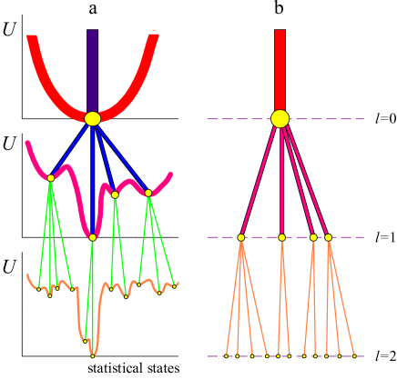
Despite a daily appearance of hierarchy in society and comprehension of its role in physical, biological, economical and other complex systems 1 -5 theory of hierarchically constrained statistical ensembles has been developed only at description of dynamics of spin glasses 6 ; 7 . Formal basis of this theory is that states of hierarchically constrained objects are related to an ultrametric space whose geometrical image is the Cayley tree with nodes corresponding to statistical (sub)ensembles 8 . The relaxation of hierarchical structures had been considered first 10a as a diffusion process on either uniformly or randomly multifurcating trees characterized by a diversity being a measure of the tree’s complexity 9a . Consequent study of the hierarchical ensembles has shown 10 their evolution was reduced to anomalous diffusion process in ultrametric space that arrives at a steady-state distribution over hierarchical levels, which is a Tsallis power law inherent in non-extensive systems 11 . Principle peculiarity of hierarchical systems consists in the splitting of each statistical ensemble residing on a given level into a number of smaller subensembles with passage onto the lower level; subsequent descent down the tree results in more small subensembles (see Fig. 1).

Figure 1: Characteristic form of the internal energy landscape (a) and related hierarchical tree (b) of complex system 15 .

From statistical point of view the set of above subensembles is characterized by the complexity, whose value determines disorder of the hierarchical coupling – in analogy with the entropy of thermodynamic systems. Formally, above quantities are defined equally, however, their physical nature is absolutely different: if the entropy characterizes disorder in distribution of primitive structural units (for example, atoms), at the complexity definition their role is played by subensembles into which the whole statistical ensemble is subdivided. Consideration of self-similar hierarchically constrained ensembles within the framework of generalized combinatorial approach shows 9 that with strengthening hierarchical coupling the complexity increases monotonically to a certain boundary value; the latter decays with both the growth of the variance of this coupling and the reduction of a branching exponent of hierarchical tree. If the last of pointed dependencies is obvious (indeed, non-branching tree does not possess a complexity), the reduction of the boundary complexity with hierarchical ensemble scattering is meant to be abnormal, as in the conventional thermodynamic ensembles the entropy always increases with temperature. Obviously, with branching change, promoting transformation of hierarchical ensemble into usual one, the pointed anomaly should be weakened and the complexity decrease with the ensemble scattering will pass into its increase.

The present work is based on generalization of the statistical approach 9 which allows, in particular, to establish the connection between the entropy of simple systems and the complexity of hierarchical ensembles. To avoid a misunderstanding, it is worth to note that the complexity introduced in Ref.9a characterizes a diversity of hierarchical tree’s themselves, whereas we are aimed to consider the disorder of hierarchically constrained ensembles in their statistical distribution over such trees. Along this line, in Section II initial statements are given to define the distribution over states of self-similar statistical ensemble and the complexity of arbitrary hierarchical system. Main results are obtained in Section III for the complexity definition within continuum approach, where the main contribution is shown to be given by the deepest levels of hierarchy. Accounting for the discrete character of distribution in Section IV shows that continuum approach derives semi-quantitative results already for several levels of hierarchy. Section V, where the complexity definition is generalized for arbitrary hierarchical ensemble, is devoted to discussion of the obtained results. Appendix contains details of generalized combinatorial approach being a basis of our consideration.

II Main statements

Generally, the behavior of a complex system is determined by the cluster structure of the whole set of hierarchical levels, however, the property of self-similarity enables one to consider a typical cluster and the level number only. As a result, the system state is described by the probability $p_{l}=p_{l}(t)$ to occupy the hierarchical level $l$ whose distribution obeys the nonlinear Fokker-Planck equation 10

$$\tau_{0}\dot{p}_{l}=-{\partial\over\partial l}\left(\epsilon p_{l}^{Q}+D{\partial p_{l}\over\partial l}\right).$$ (1)

Here, the level number $l\gg 1$ is supposed to be large to justify the use of the continuum approach, the overpoint denotes the derivative with respect to the time $t$ whose microscopic scale is $\tau_{0}$, and the diffusion coefficient $D$ represents the second moment of the intensity of transitions between microscopic states. Unlike the behavior of simple systems which is determined by the linear drift corresponding to the first moment of this intensity, the principle role in behavior of hierarchical ensembles plays the nonlinear term, fixed by both the factor $\epsilon>0$ and the exponent $Q\in[1,2]$. At the initial stage $t\ll\tau_{d}$, $\tau_{d}\equiv(\epsilon^{Q-2}/D^{Q-1})l^{Q}\tau_{0}$, the contribution of diffusion is negligible and the characteristic scale of hierarchy increases with time according to the power law $l_{c}=Q^{1/Q}(t/\tau_{0})^{1/Q}$, whereas the probability density $p_{l}(t)=(l/Q\epsilon)^{1/(Q-1)}(t/\tau_{0})^{-1/(Q-1)}$ decays hyperbolically with time. Transition to the diffusion regime $\tau_{d}\sim t\ll\tau$, $\tau\equiv l^{2}\tau_{0}$ leads to transformation of the time dependence $l_{c}(t)$ into the usual root form $l_{c}=\sqrt{2(t/\tau_{0})}$, while the probability density decays according to the same hyperbolic law. This law is appeared to be always inherent in hierarchical ensembles, being not only self-similar but also arbitrary ones 9a .

With growth of the time to macroscopic values $t\gg\tau$, the probability distribution takes the stationary Tsallis form 11

$$\begin{split}&p_{l}=\left[p_{0}^{-(Q-1)}+\frac{Q-1}{\Delta}l\right]^{-{1\over Q-1}};\\ &p_{0}\equiv\left(\frac{2-Q}{\Delta}\right)^{\frac{1}{2-Q}},\quad\Delta\equiv D/\epsilon.\end{split}$$ (2)

The probability (2) increases monotonically with $l$ decrease, i.e., with growth of hierarchical cluster, reaching the maximum value $p_{0}$ on the top level $l=0$ related to the whole system. Growth of the variance $\Delta\equiv D/\epsilon$ expands considerably the stationary distribution over hierarchical levels. Characteristically, in the limit $\Delta\gg 1$ the distribution (2) differs slightly from exponential one on high levels $l\ll\Delta^{1/(2-Q)}$, however, with passing onto deeper levels the distribution tail becomes power-law. Study of possible types of hierarchical coupling 12 has shown the distribution (2) is inherent in statistical systems related to a self-similar ultrametric space with fractal dimension $d=(Q-1)/(2-Q)$.

The statistical theory of self-similar hierarchical ensembles is based on generalization of both logarithmic and exponential functions given by expressions (A.1), being type of deformed exponential distribution (2). As shown in Appendix, the additivity condition of the logarithm function is provided by the related deformation rules for the multiplication/division operations, essentially changing the form of the usual multinomial coefficients which are the basis of combinatorial formalism of statistical physics 13 . Making use of this formalism shows 9 that connection between complexities of the nearest hierarchical levels is expressed by equality (A.15). In accordance with Fig.2

Figure 2: a) Numbers of states on nearest levels of typical hierarchical cluster; b) trivial hierarchical tree; c) parameterization of nodes on nearest levels.

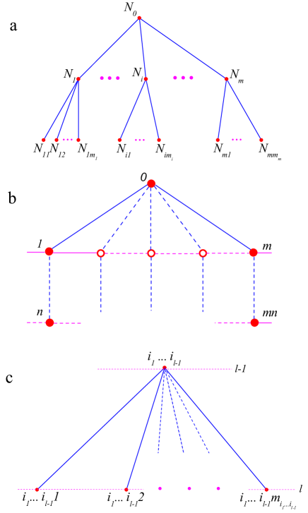
we suppose here that $N_{0}$ states of the top level are distributed over the $m$ groups on the lower level (labeled by $i$), each of which contains nodes $ij$ on the bottom level of a hierarchical cluster. If the group $i$ possesses $N_{i}$ occupied states and there are $N_{ij}$ occupied states within each set $ij$, then the corresponding probabilities take the values $p_{i}=N_{i}/N$, $p_{ij}=N_{ij}/N$, where $N$ is the total number of statistical states of hierarchical ensemble. Note that $N$ is not reduced to value $N_{0}\ll N$ related to the given cluster. Because of the obvious condition $N_{i}=\sum_{j=1}^{m_{i}}N_{ij}$, the above probabilities are connected by the equality

$$p_{i}=\sum_{j=1}^{m_{i}}p_{ij}.$$ (3)

As a result, expression (A.15), accompanied with Eqs. (A.12) (A.13), takes the form

$$\begin{split}C_{Q}\left(p_{11},\dots,p_{mm_{m}}\right)&=C_{Q}\left(p_{1},\dots,p_{m}\right)+\\ &\sum\limits_{i=1}^{m}p_{i}^{Q}C_{Q}\left(\frac{p_{i1}}{p_{i}},\dots,\frac{p_{im_{i}}}{p_{i}}\right).\end{split}$$ (4)

Here, the last factor represents relative complexity defined by the Tsallis expression

$$C_{Q}\left(\frac{p_{i1}}{p_{i}},\dots,\frac{p_{im_{i}}}{p_{i}}\right)=(Q-1)^{-1}\sum_{j=1}^{m_{i}}\left[\frac{p_{ij}}{p_{i}}-\left(\frac{p_{ij}}{p_{i}}\right)^{Q}\right].$$ (5)

Utilizing this formula we express the connection between the complexities of nearest hierarchical levels in terms of the related probability distributions over statistical states:

$$\begin{split}C_{Q}\left(p_{11},\dots,p_{mm_{m}}\right)&-C_{Q}\left(p_{1},\dots,p_{m}\right)=\\ &\frac{1}{Q-1}\sum_{i=1}^{m}\sum_{j=1}^{m_{i}}p_{ij}\left(p_{i}^{Q-1}-p_{ij}^{Q-1}\right).\end{split}$$ (6)

Above consideration concerns a typical hierarchical cluster depicted in Fig.2 . To consider the whole statistical ensemble consisting of such clusters, let us suppose that statistical states are distributed over microcanonical (sub)ensembles with probabilities and corresponding complexities defined by the level number $l$ only: $\{p_{ij}\}\Rightarrow p_{l+1}$, $\{p_{i}\}\Rightarrow p_{l}$; $C_{Q}\left(p_{11},\dots,p_{mm_{m}}\right)\Rightarrow C(l+1)$, $C_{Q}\left(p_{1},\dots,p_{m}\right)\Rightarrow C(l)$. As a result, relation (6) takes the simplest form

$$C(l+1)-C(l)=\frac{M_{l}}{Q-1}p_{l+1}\left(p_{l}^{Q-1}-p_{l+1}^{Q-1}\right).$$ (7)

For self-similar ensembles node numbers are distributed over levels $l=0,1,\dots,n$ according to the power law 12

$$M_{l}=(l+1)^{a}$$ (8)

with an exponent $a>1$. In the limit $l\gg 1$, the condition (3) takes the form

$$M_{l}p_{l}=M_{l+1}p_{l+1}.$$ (9)

Then, Eqs. (8), (9) accompanied with asymptotic behavior of distribution (2) show the self-similarity condition is fulfilled for hierarchical trees related to the branching exponent

$$a=\frac{1}{Q-1}.$$ (10)

Stationary probability distributions over states of the nearest levels are known to be connected by the recurrence relation 10

$$p_{l+1}-p_{l}=-p_{l}^{Q}/\Delta,\quad l=0,1,\dots,n.$$ (11)

In the limit $l\gg 1$, this relation is reduced to the steady-state Fokker-Planck equation (1).

III Continuum approach

Assuming that total number of levels is $n\to\infty$, let us find the complexity of hierarchical ensemble where the main contribution is given by deep levels with $l\gg 1$. Here, the statistical state probabilities of nearest levels are connected by relations

$$\begin{split}p_{l+1}^{Q-1}-p_{l}^{Q-1}&\simeq\frac{\rm d}{{\rm d}l}p_{l+1}^{Q-1}=\\ &(Q-1)p_{l+1}^{Q-2}\frac{{\rm d}p_{l+1}}{{\rm d}l}\simeq-\frac{Q-1}{\Delta}p_{l+1}^{2(Q-1)},\end{split}$$ (12)

where the last equality is written with accounting for equation (11) taken in the continuum limit. Then, substitution of Eq.(12) into Eq.(7) gives

$$C(l+1)-C(l)\simeq\frac{M_{l}}{\Delta}p_{l+1}^{2Q-1}.$$ (13)

Rewriting $C(l+1)-C(l)$ in the continuum limit as ${\rm d}C/{\rm d}l$ and taking into account Eqs. (2), (8) allow one to reduce the difference equation (13) to the following differential equation,

$$\frac{{\rm d}C}{{\rm d}l}=\frac{l^{a}}{\Delta}\left[p_{0}^{-(Q-1)}+\frac{Q-1}{\Delta}~{}l\right]^{-{2Q-1\over Q-1}},$$ (14)

where $l+1$ is replaced with $l$.

In the limiting case $a\to 1$, solution of Eq.(14) leads to the dependence

$$C(n)=\frac{\Delta}{Q}p_{0}\left[1-\left(\frac{p_{n}}{p_{0}}\right)^{Q}\right]-np_{n}^{Q}.$$ (15)

Here, the complexity appears to be the monotonically increasing function of the level number $n$. It has the initial value $C(0)=0$ and the maximum value

$$C(\infty)=\frac{(2-Q)^{\frac{1}{2-Q}}}{Q}\Delta^{-\frac{Q-1}{2-Q}},$$ (16)

decaying with growth of both the non-extensivity parameter $Q$ and the variance $\Delta$. Remarkably, the complexity obtained here behaves similarly to that found in our recent work 9 . However, the analogous expressions (16)-(18) appearing in Ref. 9 are much more complicated than the equalities (14)-(16) derived in this section. It is accounted for that continuum approach has been already used in Ref.9 at estimation of the relative entropy (5), whereas in the present study we pass to continuum limit at a later stage, while defining probability difference (12) to estimate the complexity difference (7). At the same time, no approximations have been imposed to express the entropy (5). The pointed distinction resulted in the exponent of the distribution function derived in Ref.9 (see the r.h.s. of Eq.(16) therein) to exceed the exponent value in Eq.(14) of this section by the magnitude $Q-1<1$. This fact, however, does not play a principle role within our approach.

At arbitrary values $a$ of the branching exponent, solution of equation (14) is expressed by means of the hypergeometric function:

$$\begin{split}C(n)=\frac{p_{0}^{2Q-1}}{\Delta}\frac{n^{1+a}}{1+a}~{}&F\left(\frac{2Q-1}{Q-1},1+a;2+a;-\nu n\right),\\ &\nu\equiv\frac{Q-1}{\Delta}p_{0}^{Q-1}.\end{split}$$ (17)

The analysis of r.h.s. of Eq.(14) shows that its solution holds finite values in the limit $n\to\infty$ if the exponent $a$ does not exceed the maximum value

$$a_{max}=\frac{Q}{Q-1}.$$ (18)

As shown above, the self-similarity condition leads to the lower value (10) for $a$, at which odd arguments of the hypergeometric function coincide and one arrives at the binomial form 14

$$F\left(\frac{2Q-1}{Q-1},\frac{Q}{Q-1};\frac{2Q-1}{Q-1};-\nu n\right)=\left(1+\nu n\right)^{-\frac{Q}{Q-1}}.$$ (19)

As a result, the complexity (17) is expressed by the simple equation

$$C(n)=\frac{Q-1}{Q}\frac{p_{0}^{Q-1}}{\Delta}p_{n}^{Q}n^{\frac{Q}{Q-1}}.$$ (20)

As for the degenerate tree ($a\to 1$), the complexity increases monotonically with the number of hierarchical levels to the maximum value

$$C(\infty)=\frac{(2-Q)^{\frac{Q-1}{2-Q}}}{Q(Q-1)^{\frac{1}{Q-1}}}\Delta^{\frac{Q+|Q_{-}|}{(Q-1)(2-Q)}(Q_{+}-Q)},$$ (21)

where roots $Q_{\pm}\equiv(1\pm\sqrt{5})/2$ represent the gold mean. With growth of the non-extensivity parameter $Q$, the maximum complexity decreases monotonically from infinite value at $Q=1$ to zero at $Q=2$. However, unlike Eq.(16), the complexity dependence on the variance $\Delta$ becomes non-monotonic: at values of the non-extensivity parameter limited to the top magnitude $Q_{+}\simeq 1.618$, the maximum complexity increases with $\Delta$ growth, whereas at $Q>Q_{+}$ it decreases. With accounting for the self-similarity condition (10), this means that behavior inherent in simple statistical systems is realized at the branching exponent of hierarchical tree exceeding gold mean $a_{+}\equiv(\sqrt{5}+1)/2\simeq 1.618$; on the other hand, the complexity decay with the variance growth, what is characteristic for complex systems, is shown to appear at values of the branching exponent within the domain $1<a<1.618$.

IV Discrete hierarchical levels

For hierarchical systems possessing a finite number of levels $n>1$, the above results of the continuum approach lose accuracy, and we need to take into account the discretization of hierarchical statistical ensemble. Probability distribution of such ensemble is defined by the set of equations (11), whose number $n$ is less by one than number of probabilities $p_{l}$, $l=0,1,\dots,n$. The ensemble description is reached by adding to the system (11) the normalization condition

$$\sum\limits_{l=0}^{n}p_{l}=1.$$ (22)

Numerical solution of Eqs. (11), (22) arrives at the probability distributions over hierarchical levels with different variances, as shown in Fig.3 (for convenience we

Figure 3: Probability distributions over hierarchical levels within representations of both half-logarithmic (a) and log-log (b) axes at $Q=1.5$ (curves 1 – 6 relate to values $\Delta=0.9,1.25,2.0,3.0,4.0,6.0$, respectively).

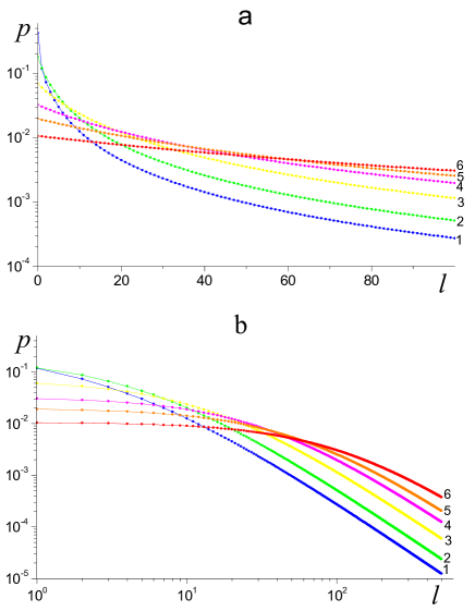
use both half-logarithmic axes, where exponential dependencies are straightened, and logarithmic axes, representing power laws with straight lines). As Fig.3a shows, distributions of statistical states over hierarchical levels are far from exponential dependencies at all values of the variance $\Delta$. The pronounced curve straightening in Fig.3b indicates the transition into power-law regime in the limit $l\to\infty$. The latter is confirmed by comparing the distribution

Figure 4: Comparison of the distribution function (2) found within continuum approach (solid lines) with solution of the difference equations (11) and the normalization condition (22) (points) at $Q=1.5$, $\Delta=1$ (a) and $Q=1.5$, $\Delta=5$ (b).

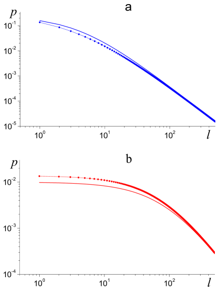
function (2) derived in the continuum limit with the solution of the system of difference equation (11) subject to the normalization condition (22). As illustrated in Fig.4, both approaches produce virtually the same results for the deep levels $l\gg 1$, however, the discrepancy at lower level numbers becomes bigger as the variance $\Delta$ increases.

The most precise representation of accuracy of the continuum approach is reached if one expresses the distribution over hierarchical levels in the modified Tsallis form

$$\begin{split}&p_{l}=\left[p_{0}^{-(Q-1)}+\frac{\alpha_{l}}{\Delta}l\right]^{-{1\over\alpha_{l}}};\\ &p_{0}\equiv\left(\frac{2-Q}{\Delta}\right)^{\frac{1}{2-Q}},\quad 0\leq l\leq n\end{split}$$ (23)

with the exponent $\alpha_{l}$ taking the value $\alpha_{l}\simeq Q-1$ in the limit $l\to\infty$. As Fig.5 shows, the continuum approach is improved by

Figure 5: Dependencies of the exponent of distribution (23) on the level number at $\Delta=1$ (a), $\Delta=2$ (b) and $Q=1.5$ (c) (numbers near curves point to values $Q$ in panels (a), (b) and $\Delta$ in (c)).

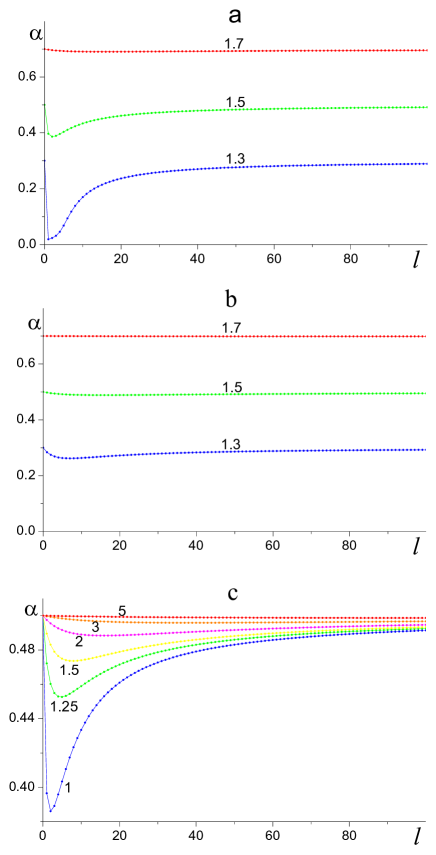
both the tendency of the non-extensivity parameter $Q$ to the limit value $Q=2$ and the unlimited growth of the variance $\Delta$. In particular, $Q\to 2$ means that branching exponent (10) tends to the limit $a=1$ related to the degenerate hierarchical tree, where the statistical ensemble is defined by hyperbolic distribution with the exponent $\alpha_{l}\simeq Q-1\to 1$. Respectively, growth of the variance increases the disorder of statistical ensemble dramatically and the discrete nature of the ensemble becomes inessential.

As in stationary case, evolution of the probability distribution over hierarchical levels is determined by the system of equations (11) along with the normalization condition (22). The number of the deepest level is defined by the diffusion law $n=\sqrt{2(t/\tau_{0})}$ (for the sake of simplicity, we accept the condition $\tau_{d}/\tau\ll 1$ for characteristic time scales, when the contribution of abnormal drift is negligible). Corresponding time dependencies of the probability distribution functions are depicted in Fig.6.

Figure 6: Evolution of the probability distribution over hierarchical levels at $Q=1.5$ and $\Delta=3$ (curves 1 – 4 relate to the time moments $t/\tau_{0}=50,1.25\cdot 10^{3},5\cdot 10^{3},5\cdot 10^{5}$, respectively).

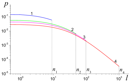
It is demonstrated how diffusion process over levels of the hierarchical tree provides relaxation to the stationary distribution shown in Fig.4.

Let us proceed now with definition of the complexity. Taking successfully values $l=0,1,\dots,n$ for the number of levels in Eq.(7), with accounting for Eqs. (8), (10), one obtains

$$C(n)=\frac{1}{Q-1}\sum_{l=1}^{n}l^{1/(Q-1)}p_{l}\left(p_{l-1}^{Q-1}-p_{l}^{Q-1}\right).$$ (24)

As shown in Fig.7, with strengthening hierarchical coupling the

Figure 7: Dependence of the complexity on the number of hierarchical levels at $Q=1.3$ (a), $Q=1.5$ (b) and $Q=1.7$ (c) (numbers near curves point to the $\Delta$ values).

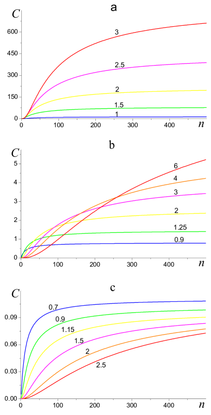
complexity grows monotonically to the maximum value which decays to zero as the non-extensivity parameter $Q$ tends to the upper border $Q=2$. What about the complexity dependence on the variance $\Delta$, it is much more complicated: at small values of $Q$ the $\Delta$-growth promotes the complexity-increase, whereas at large $Q$ the complexity decreases with the variance. Fig.8 demonstrates this peculiarity

Figure 8: Dependence of complexity on variance for levels $n=500$ at $Q=1.50$ (a), $Q=1.65$ (b) and $Q=1.70$ (c).

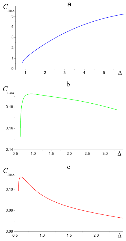
representing the complexity as a function of variance $\Delta$ for a large number of levels $n=500$ and different values of $Q$. It is seen that complexity increases monotonically with $\Delta$ at small $Q$, decays at large $Q$ and varies non-monotonically at intermediate $Q$.

According to consideration of the previous Section, such complexity behavior is also captured by the relation (21). The latter, in particular, implies that the maximum complexity as a function of variance exhibits the behavior inherent in simple statistical systems at values of non-extensivity parameter limited from above by the gold mean $Q_{+}\simeq 1.618$. On the other hand, at $Q>Q_{+}$ the variance-growth reduces the complexity of hierarchical ensemble. Qualitatively, such complexity dependence can be perceived while considering a trivial hierarchical tree (see Fig.2b) in line with the following reasonings. As the top node splits into $m>1$ parallel branches, each of which comprises of $n>1$ sub-nodes, the total number of nodes equals $N=1+mn$; at that, the top node relates to the probability $p_{0}=m/N$, whereas each of the remaining sub-nodes is associated with the probability $p=1/N$. Then, the complexity definition (24) gives the value $C_{1}=(Q-1)^{-1}p(p_{0}^{Q-1}-p^{Q-1})$ for each of the tree branches and the total complexity $C=mC_{1}$ takes the value

$$C=(Q-1)^{-1}\frac{1-m^{-(Q-1)}}{(n+m^{-1})^{Q}}\sim n^{-Q}.$$ (25)

As one would expect, the latter grows with increase of the branching $m$ and reduction of the length of branches $n$. Since for a stochastic tree the $n$-growth is attributed to the increase in disorder of states over levels, the estimation (25) provides an explanation for an abnormal decay of the complexity with growth of the variance of hierarchical ensembles – it is caused by the increase in number of subensembles which are connected with each other without hierarchical constraining.

Characteristic peculiarity of the curves depicted in Fig. 8 is their break at small variance, where the complexity (24) becomes ill-defined. Such behavior is caused by the functional form of the distribution (2), implying that the decrease in variance $\Delta$ leads to unlimited growth of the probability to occupy the top level $p_{0}\propto\Delta^{-1/(2-Q)}$. Therefore, at small $\Delta$ the maximum probability $p_{0}=1$ is reached, so the whole hierarchical system accumulates on the top level and the definition of complexity loses sense.

Comparison between the complexities (24) and (20) defined within discrete and continuum approaches, respectively, is shown in Fig.9.

Figure 9: Comparison of complexities (24) determined within both discrete (solid lines) and continuum (dashed lines) approaches: a) $Q=1.5$ (curves 1 – 3 relate to $\Delta=1,2,3$, respectively); b) $Q=1.7$ (curves 1 – 3 relate to $\Delta=0.7,0.9,1.2$, respectively).

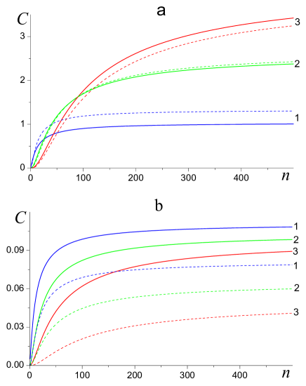
It is seen that both approaches result in the identical complexity dependence on the number of hierarchical levels $n$. However, with growth of the non-extensivity parameter $Q$ the continuum approach loses the accuracy. Such behavior is rationalized by the reduction of the tree branching with $Q$-growth, promoting enhanced contribution of top levels where the continuum approach is inapplicable.

Time dependence of the complexity $C(t)$ is defined by evolution of the probability distribution $p_{l}(t)$ over hierarchical levels. Fig.6 shows that in the course of time the level variance is strengthened, so, accordingly, the dependence $C(t)$ should have the same form as the complexity variation with the $\Delta$ variance growth for stationary case (see Fig.8). Indeed, as indicated in Fig.10, complexity increases with time the faster, the greater the distribution scattering, provided the non-extensivity parameter does not exceed the gold mean $Q_{+}\simeq 1.618$ 9 .

Figure 10: Time dependencies of the complexity at $Q=1.5$ (a) and $Q=1.7$ (b); curves 1 – 3 relate to values $\Delta=1,2,3$ (a) and $\Delta=0.7,0.9,1.2$ (b), respectively.

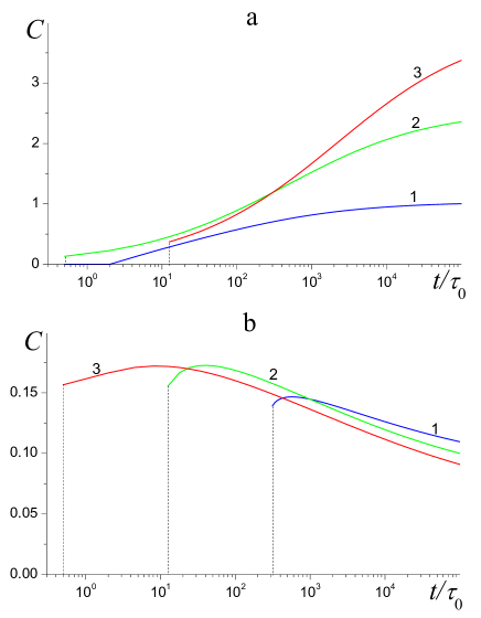
However, at $Q>Q_{+}$ the system evolution becomes abnormal: a short-term increase of the complexity from finite values is followed by its long-continued decay to the values decreasing with the $\Delta$ variance growth.

V Discussion

Above consideration is based on the definition of microcanonical ensemble, where the probabilities $p_{i_{1}\dots i_{l}}$ to occupy statistical states $i_{1}\dots i_{l}$ on $l$th hierarchical level take equal values $p_{l}\sim p_{0}/M_{l}$ defined by the condition (9). According to Eq.(8), these probabilities decay with $l$-growth due to increase in the number of states $M_{l}$. As a result, the recurrence relation (6) is reduced to simple equality (7), whose iteration gives the expression (24) for the complexity of the self-similar hierarchical ensemble.

In general case of arbitrary distribution over nodes of the hierarchical tree, not possessing the property of self-similarity, the difference equation (6) leads to the complicated expression

$$\begin{split}&C(n)=\frac{1}{Q-1}\sum_{l=1}^{n}C_{l},\\ C_{l}\equiv&\sum_{i_{1}=1}^{m}\sum_{i_{2}=1}^{m_{i_{1}}}\dots\sum_{i_{l}=1}^{m_{i_{1}i_{2}\dots i_{l-1}}}p_{i_{1}\dots i_{l-1}i_{l}}\times\\ &\left(p_{i_{1}\dots i_{l-1}}^{Q-1}-p_{i_{1}\dots i_{l-1}i_{l}}^{Q-1}\right),\end{split}$$ (26)

where the probability $p_{i_{1}\dots i_{l-1}}$ is reduced to the value $p_{0}$ at $l=1$. In contrast to a simple two-level tree depicted in Fig.2 , it is meant here that on the level $l$ of the hierarchical tree comprised of $n>1$ total number of levels the set of states $i_{1}\dots i_{l-1}1$, $i_{1}\dots i_{l-1}2$, $\dots$, $i_{1}\dots i_{l-1}m_{i_{1}i_{2}\dots i_{l-1}}$ forms a cluster related to the node $i_{1}\dots i_{l-1}$ on the upper level $l-1$ (see Fig.2c). Therefore, to calculate the complexity (26), one needs first to sum over the nodes $i_{1}\dots i_{n-1}i_{n}$ of the bottom level $n$, which belong to the cluster related to the node $i_{1}\dots i_{n-1}$ of the upper level $n-1$. Then, the summation over nodes of the level $n$ belonging to all remaining clusters is carried out and the same procedure is repeated for each subsequent hierarchical level $l<n$ .

Expression (26) is a basis for the numerical definition of the complexity of arbitrary hierarchical ensemble (for example, in case of the complex defect structure of solids subject to intensive external influence type of strong plastic deformation or rigid radiation treatment). Unlike the amorphous systems, the number of structure levels of a real crystal is rather not large. Particularly, among different spatial scales in the latter type of systems, it is accepted to distinguish between several basic levels of consideration 15 . The finest level, the microscopic one, is related to homogeneous distribution of point defects, dislocation and disclination. Next, the coarser mesoscopic level corresponds to homogeneously distributed structure cells and fragments. Finally, the macroscopic objects such as homogeneously distributed grains and texture components are considered on a macroscopic level. To define the complexity of a real structure, one needs first to distribute the whole ensemble of defects over hierarchical levels $l=0,1,\dots,n$, then to calculate on each of them a number of defects $N_{i_{1}\dots i_{l-1}}$ belonging to the cluster $i_{1}\dots i_{l-1}1$, $i_{1}\dots i_{l-1}2$, $\dots$, $i_{1}\dots i_{l-1}m_{i_{1}i_{2}\dots i_{l-1}}$, and, finally, to attribute the probability

$$p_{i_{1}\dots i_{l-1}}=\frac{N_{i_{1}\dots i_{l-1}}}{N}$$ (27)

to the node $i_{1}\dots i_{l-1}$ of the upper level $l-1$. At that, the total number of defects residing on all levels is defined as

$$N=\sum_{i_{1}=1}^{m}\sum_{i_{2}=1}^{m_{i_{1}}}\dots\sum_{i_{n}=1}^{m_{i_{1}\dots i_{n-1}}}N_{i_{1}\dots i_{n}},\quad n>1$$ (28)

where $m_{i_{1}\dots i_{l-1}}$ is the number of possible states $i_{1}\dots i_{l}$ within the cluster related to the node $i_{1}\dots i_{l-1}$ (at $n=1$ one has $m_{i_{1}\dots i_{n-1}}=m$) . Substitution of the obtained set of probabilities $\left\{p_{i_{1}\dots i_{l}}\right\}$, $l=0,1,\dots,n$ into Eq.(26) gives the complexity of hierarchically constrained defect structure of a solid. Obviously, this complexity determines such phenomenological quantities as strength and plasticity of solid. Remarkably, such definition of the structural complexity cannot be reached solely by means of experimental methods (for example, electron microscopy), but requires a subsequent computer processing according to the above algorithm.

Realization of the described program, however, represents rather a challenge. Therefore, in the preceding sections we limited ourselves to considering a self-similar hierarchical tree characterized by the level number $n$ and a typical cluster with the branching exponent $a$. Studying the various hierarchical trees has revealed three their types 12 : (1) the degenerate tree possessing only one branching node per level, so the total number of nodes increases linearly with $n$; (2) the regular tree, where on each level all nodes branch equally, and the total node number increases exponentially with $n$; and (3) the self-similar irregular tree characterized by the power law (8) with exponent $a>1$ for the $l$-dependence of the number of nodes. In the first two cases the probabilities of state occupation on various hierarchical levels vary logarithmically slow and exponentially fast, respectively, while in the last case it obeys the power-law dependence (2) inherent in the self-similar systems. According to Eq.(10), the non-extensivity parameter $Q=(a+1)/a$ is determined by the branching exponent $a$: regular $(a=\infty)$ and degenerate $(a=1)$ trees are characterized by limiting values $Q=1$ and $Q=2$, respectively, whereas the power-law distribution (2) with exponent $1<Q<2$ takes place at $\infty>a>1$.

As pointed in Introduction, the complexity of different hierarchical trees has been first considered in works 10a , 9a . Within our notation, these trees have been characterized with the silhouette

$$s_{l}:=\ln\frac{M_{l}}{M_{l-1}}$$ (29)

that determines the logarithmic growth rate of the node number $M_{l}$ with increase of the hierarchical level number $l$. A peculiarity of the approach used in Ref.10a is that it is based on the consideration of the regular tree, whose nodes are multifurcated with the constant branching index $b>1$. In this case, one has the dependence $M_{l}=b^{l}$ and the definition (29) gives a simple relation $s=\ln b$. However, for the main object of our consideration, a self-similar tree, Eq. (8) for the number node distribution has to be used, and the resulting silhouette $s_{l}=\ln\left(1+1/l\right)^{a}\simeq a/l$ depends significantly on the level number even in the continuum limit $l\gg 1$. It is clear that such $l$-dependence is caused by the definition (29) introduced for trees related to the regular ones, whereas self-similar irregular trees represent their antipode. Obviously, the silhouette of a self-similar tree may be defined with the equalities

$$s:=\frac{M_{\lambda l}-M_{l}}{(\lambda-1)M_{l}}=[a]_{\lambda},\quad[a]_{\lambda}\equiv\frac{\lambda^{a}-1}{\lambda-1}.$$ (30)

This definition is based on use of the Jackson derivative which determines the variation rate of the function (10) with respect to the dilatation $\lambda\geq 1$ and reduces to the usual derivative in the limit $\lambda\to 1$ Jackson . According to Eq.(29), the silhouette of self-similar tree is the $\lambda$-basic number $[a]_{\lambda}$, whose value equals the exponent $a$ at the limit dilatation value $\lambda=1$ and grows as $\lambda^{a-1}$ at $\lambda\gg 1$. Obviously, the present study of self-similar hierarchical ensembles relates to the first case, $\lambda=1$.

In summary, our study indicates that formation of hierarchical coupling promotes a fast complexity growth to a certain maximum value. With strengthening of the branching parameter $a$ of hierarchical tree the maximum complexity grows monotonically from zero at $a=1$ to infinity at $a\to\infty$. Investigating the variance-dependence of the complexity has revealed a behavior inherent in simple systems at the values of branching exponent exceeding the gold mean $a_{+}=1.618$. On the other hand, the complexity-decrease with the variance-growth, being a characteristic of complex systems, has been observed for the range $1<a<1.618$ of the branching exponent.

Appendix

As known, the non-extensive statistical mechanics is based on the following definitions for logarithmic and exponential functions 11 ,

$$\ln_{q}(x):=\frac{x^{1-q}-1}{1-q},\ \exp_{q}(x):=\left[1+(1-q)x\right]_{+}^{1\over 1-q};\quad[y]_{+}:=\max(0,y),\ q\leq 1,$$ (A.1)

which are reduced to the usual functions in the limit $q\to 1$. Introducing the $q$-deformed multiplication and division operations for the positive values $x,y$ as follows,

$$x\otimes_{q}y=\left[x^{1-q}+y^{1-q}-1\right]_{+}^{1\over 1-q},\ x\oslash_{q}y=\left[x^{1-q}-y^{1-q}+1\right]_{+}^{1\over 1-q};\quad x,y>0,$$ (A.2)

it is easy to verify that they satisfy the usual properties

$$\begin{split}&\ln_{q}(x\otimes_{q}x)=\ln_{q}x+\ln_{q}y,\quad\ln_{q}(x\oslash_{q}x)=\ln_{q}x-\ln_{q}y;\\ &\exp_{q}(x)\otimes_{q}\exp_{q}(y)=\exp_{q}(x+y),\quad\exp_{q}(x)\oslash_{q}\exp_{q}(y)=\exp_{q}(x-y)\end{split}$$ (A.3)

of the logarithmic and exponential functions.

Within combinatorial approach 13 , the $q$-deformed statistics is reduced to consideration of the generalized factorial $N!_{q}:=1\otimes_{q}\dots\otimes_{q}N$ and the corresponding logarithm,

$$\ln_{q}(N!_{q})=\frac{\sum_{i=1}^{N}i^{1-q}-N}{1-q}.$$ (A.4)

In the thermodynamic limit $N\to\infty$, a sum in the above equation is replaced by an integral, and one gets

$$\ln_{q}(N!_{q})=\left\{\begin{array}[]{ll}\frac{N}{2-q}\ln_{q}N-\frac{N}{2-q}+{\it O}(\ln_{q}N),\qquad q\neq 2,\\ N-\ln N+{\it O}(1),\quad\quad\quad\quad\quad\quad\quad q=2.\end{array}\right.$$ (A.7)

Defining $q$-deformed multinomial coefficient as

$${N\choose N_{1}\dots N_{k}}_{q}:=(N!_{q})\oslash_{q}\left[(N_{1}!_{q})\otimes_{q}\dots\otimes_{q}(N_{k}!_{q})\right]$$ (A.8)

with a set of integers $N_{i}$ subject to the condition $N=\sum_{i=1}^{n}N_{i}$, we find

$${N\choose N_{1}\dots N_{k}}_{q}=\left[\sum\limits_{i=1}^{N}i^{1-q}-\sum\limits_{i_{1}=1}^{N_{1}}i_{1}^{1-q}-\dots-\sum\limits_{i_{k}=1}^{N_{k}}i_{k}^{1-q}+1\right]_{+}^{1/(1-q)}.$$ (A.9)

Similarly to Eq.(A.7), the logarithm

$$\ln_{q}{N\choose N_{1}\dots N_{k}}_{q}\simeq\left\{\begin{array}[]{ll}\frac{N^{2-q}}{2-q}C_{2-q}\left(\frac{N_{1}}{N},\dots,\frac{N_{k}}{N}\right),\qquad q>0,q\neq 2,\\ -C_{1}(N)+\sum\limits_{i=1}^{k}C_{1}(N_{i}),\quad\quad\quad\quad\quad\quad q=2\end{array}\right.$$ (A.12)

is calculated to construct a Tsallis entropy

$$C_{Q}(p_{1},\dots,p_{N}):=-\sum\limits_{i=1}^{N}p_{i}\ln_{2-Q}(p_{i})=\frac{\sum_{i=1}^{N}p_{i}^{Q-1}-1}{Q-1}$$ (A.13)

related to the physical parameter $Q\equiv 2-q\geq 1$.

The above formalism can be easily generalized to study hierarchical systems 16 . To this end, let us consider a structure of the hierarchical ensemble comprised of $N$ states. These states are distributed over subensembles $i=1,\dots,m$, each containing $N_{i}$ states. In turn, every of these subensemble further splits in $m_{i}$ smaller subensembles $ij$, each possessing $N_{ij}$ states. As the ensemble states are distributed, the relations $\sum_{j=1}^{m_{i}}N_{ij}=N_{i}$, $\sum_{i=1}^{m}N_{i}=N$ hold. Then, expression (A.8) for the multinomial coefficients takes a generalized form,

$${N\choose N_{11}\dots N_{mm_{m}}}_{q}={N\choose N_{1}\dots N_{m}}_{q}\otimes_{q}{N_{1}\choose N_{11}\dots N_{1m_{1}}}_{q}\otimes_{q}\dots\otimes_{q}{N_{m}\choose N_{m1}\dots N_{mm_{m}}}_{q},$$ (A.14)

whose $q$-logarithm is

$$\ln_{q}{N\choose N_{11}\dots N_{mm_{m}}}_{q}=\ln_{q}{N\choose N_{1}\dots N_{m}}_{q}+\sum\limits_{i=1}^{m}\ln_{q}{N_{i}\choose N_{i1}\dots N_{im_{i}}}_{q}.$$ (A.15)

Applying the estimation (A.12) to the last formula arrives at the connection (4) between the complexities of the nearest hierarchical levels.

VI Acknowledgements

We are grateful to Dr. B.A. Huberman for bringing to our attention Refs. 10a , 9a related to the addressed issues. We also thank Dr. A.P. Savelyev for helpful discussions and careful manuscript reading.

References

- (1) J.S. Nicolis, Dynamics of Hierarchical Systems (An Evolutionary Approach) (Springer-Verlag, Berlin, Heidelberg, 1986).
- (2) A.I. Olemskoi, in Physics Reviews 18, Part 1, Ed. I.M. Khalatnikov (Gordon & Breach, London, 1996).
- (3) K. Mainzer, Thinking in Complexity (Springer-Verlag, Berlin, 1997).
- (4) R.N. Mantegna, H.E. Stanley, An introduction to econophysics. Correlations and complexity in finance (Cambridge University Press, Cambridge, 1999).
- (5) P. Holme, M. Huss, H. Jeong, Bioinformatics 19, 532 (2003).
- (6) M. Mezard, G. Parisi, M.A. Virasoro, Spin Glass Theory and Beyond (World Scientific, Singapur, 1987).
- (7) V.S. Dotsenko, Physics-Uspekhi 163, No.6, 1 (1993).
- (8) R. Rammal, G. Toulouse, M.A. Virasoro, Rev. Mod. Phys. 58, 765 (1986).
- (9) C.P. Bachas, B.A. Huberman, Phys.Rev.Lett. 57 , 1965 (1986).
- (10) B.A. Huberman, T. Hogg, Physica D 22, 376 (1986).
- (11) A.I. Olemskoi, JETP Letters 71, 285 (2000).
- (12) M. Gell-mann, C. Tsallis, Nonextensive Entropy: Interdisciplinary Applications (Oxford University Press, Oxford, 2004).
- (13) A.I. Olemskoi, Theory of Structure Transformations in Non-Equilibrium Condensed Matter (NOVA Science, New York, 1999).
- (14) A.I. Olemskoi, JETP Letters 85, 137 (2007).
- (15) A.I. Olemskoi, A.D. Kiselev, Phys. Lett. A 47, 221 (1998).
- (16) H. Suyari, Physica A 368, 63 (2006).
- (17) M. Abramowitz, I.A. Stegun, Handbook of Mathematical Functions (Dover, New York, 1972).
- (18) M. Arik, in Symmetries in Science VI: From to Rotation Group to Quantum Algebras (Plenum Press, New York, 1993).
- (19) H. Suyari, T. Wada, arXiv:cond-mat/0608007.