Shapes of Semiflexible Polymers in Confined Spaces

Abstract

We investigate the conformations of a semiflexible polymer confined to a square box. Results of Monte Carlo simulations show the existence of a shape transition when the persistence length of the polymer becomes comparable to the dimensions of box. An order parameter is introduced to quantify this behavior. A simple mean-field model is constructed to study the effect of the shape transition on the effective persistence length of the polymer.

I Introduction

Biological macromolecules live in the crowded, confined environment of a cell. They are often packed into spaces that are much smaller than their natural size and adopt conformations which are unlikely to occur in free space. For example, viral DNA is packaged in a capsid whose dimensions are comparable to the persistence length of DNA J.Kindt et al. (2001); Odijk (2004); Ali et al. (2004); Jiang et al. (2006); E.Katzav et al. (2006), which obliges the DNA to adopt a tightly bent shape. Other examples of strong confinement include actin filaments in eukaryotic cell Köster et al. (2007), and protein encapsulated in E.Coli G.Morrison and Thirumalai (2005). In such environments, the macromolecule is forced to optimize the competing demands of configurational entropy, excluded volume and bending energy. The packaging of DNA in viral capsids has been investigated extensively and illustrates the effects of these competing interactions and the additional electrostatic forces arising from its charged nature J.Kindt et al. (2001); Odijk (2004). Experimental and theoretical studies Ali et al. (2004); Muthukumar (2001); A. Arnold and et al (2007) show that the static, and dynamic properties such as threshold force for packaging and packaging time, change drastically with changes in confining geometry. Another example is provided by driving DNA through a nanochannel by electrical force Matysiak et al. (2006); Slonkina and Kolomeisky (2003), where the dimensions of the channel determine the translocation time and threshold voltage. Understanding the statistics of polymer in confinement is therefore essential for exploring both the static and dynamic properties of DNA Sakaue and Raphaël (2006).

In this paper, we investigate the shape and rigidity of a single, semiflexible polymer under confinement. Using the Bond-Fluctuation-Model (BFM) Carmesin and Kremer (1988), we simulate a single, semiflexible polymer chain confined to a box in two dimensions. One advantage of the two-dimensional (2D) simulations is that they can be compared directly to experimental measurements, since conformations of DNA on a substrate can be visualized through atomic force microscopy (AFM) which characterize the statistics of fluctuations of DNAMoukhtar et al. (2007). Our simulations show that there is a shape transition as a function of increasing rigidity. We analyze the nature of this transition by defining an order parameter associated with the transition. As expected, the flexibility of the chain, measured by the tangent-tangent correlation function, evolves with the shape change. We construct a theory for this correlation function by considering Gaussian fluctuations around the “average shape”.

II Simulations

The simulations are performed using the bond fluctuation algorithm, introduced by Kremer and Carmersin Carmesin and Kremer (1988). The bond fluctuation model (BFM) is a coarse-grained model of a polymer in which the chain lives on a hypercubic lattice and fluctuations on scales smaller than the lattice constant are suppressed. The polymer is represented by a chain of effective monomers connected by effective bonds. The effective bonds and effective monomers are constructed to account for excluded volume effects. In 2D, each monomer occupies an elementary square and forbids other monomers to occupy its nearest and next-nearest neighbors Baschnagel and Binder (1995). In order to avoid crossing of bonds, the effective bonds are restricted to the set:

$$B=P(2,0)\cup P(2,1)\cup P(2,2)\cup P(3,0)$$

$$\cup P(3,1)\cup P(3,2)$$ (1)

in units of lattice spacing, and $P(m,n)$ stands for the sign combinations $\pm m,\pm n$ and all the permutations. With this restriction, the average bond length (Kuhn length b) is 2.8. Fig. 1 illustrates the BFM representation of a polymer and shows one allowed move that obeys the self-avoidance condition.

Figure 1: One configuration of polymer in BFM. The bond vectors are restricted to the set B (Eq. 1) and one possible move is denoted by the dashed line.

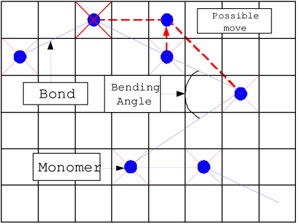
The only non-bonded interaction included in this representation is excluded volume. To represent a semiflexible polymer, such as DNA in this model, the energy cost of bending has to be incorporated. The mechanical properties of DNA are well described by the worm-like chain model (WLC) Yamakawa (1971), in which DNA is characterized by its total contour length $L$ and persistence length $l_{p}$. In the continuum limit, the bending energy $H_{b}$ in D-dimensional space can be expressed as:

$$H_{b}=\frac{\kappa}{2}\int_{0}^{L}\bigl{[}\frac{d\mathbb{u}(s)}{ds}\bigr{]}^{2}\,ds$$ (2)

where the stiffness, $\kappa$, is related to $l_{p}$ by $\frac{\kappa}{k_{B}T}=\frac{D-1}{2}l_{p}$, and $l_{p}$ characterizes the decay length of the correlation between the tangent vectors Yamakawa (1971)

$$\langle\mathbb{u}(s)\cdot\mathbb{u}(0)\rangle\propto e^{-\frac{s}{l_{p}}}~{}.$$ (3)

Here $\mathbb{u}(s)=\partial\mathbb{R}(s)/\partial{s}$ is the tangent vector at arclength s, and $\mathbb{R}(s)$ is the position vector. The effect of confinement on the form of this correlation function is one of the questions we explore in this paper. In the following, all energies will be measured in units of $k_{B}T$.

In a lattice representation such as the BFM, the bending energy $H_{b}$ associated with a configuration is expressed as Wilhelm and Frey (1996):

$$H_{b}=\frac{l_{p}}{2b}\sum_{i=1}^{N-1}\mathbb{u}_{i}\cdot\mathbb{u}_{i+1}$$

where $N$ is the total number of monomers in the chain. The modified BFM model now includes excluded volume interactions and bending rigidity. Monte Carlo calculations are carried out using the Metropolis Algorithm with $H_{b}$ as the energy function since excluded volume effects are incorporated in the allowed configurations of the BFM.

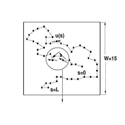
Fig. 2 illustrates the simulation setup for a semiflexible chain in a square box with linear dimension $W$, in which all lengths are measured in units of the Kuhn length. The radius of gyration $R_{g}$ of the unconfined semiflexible chain is proportional to $L^{\nu}l_{p}^{1-\nu}$ Liu and Chakraborty (2006), where $\nu$ is the Flory exponent ($\nu=\frac{3}{4}$ for 2D, $\nu\approx 0.588$ for 3D Doi and Edwards (1986)) . We set up conditions such that $R_{g}$ is larger than the box size. For a chain of contour length $L=60$, $W$ has to be less than $21.5$, for this condition to be met. Most of our results were obtained for $L=60$ and $W=15$, however, limited sets of data were also collected for $L=80$, $W=15$ and $L=40$, $W=10$ to investigate the effects of $L$ and $W$. In addition, we compare the results of a circular box to a square box. Each Monte Carlo trajectory is allowed to equilibrate for $10^{9}$ Monte Carlo steps which correspond to many ($\sim 100$) Rouse relaxation times Doi and Edwards (1986). The range of the persistence length $l_{p}$ is varied from 0, corresponding to a flexible chain, up to $W$, which is the rod-like limit. For each $l_{p}$, more than 20 independent runs were performed to get adequate statistics.

Figure 2: $(a)$ One initial configuration of our simulation. The contour length of the chain is 60, box size is 15. $\mathbb{u}(s)$ is illustrated by arrows. $(b)$ Mapping part of the chain circled in $(a)$ onto $\mathbb{u}(s)$ space.

III Shapes in confinement

For a semiflexible chain, the mechanical properties are well described by a self-avoiding walk Valle et al. (2005), and the only effect of the semiflexibility is to change the Kuhn length Liu and Chakraborty (2006). In confinement, especially if the confining dimensions are smaller than or comparable to the persistence length, semiflexibility plays a much more important role since the bending energy is in intense competition with the entropy. As a result, the conformations adopt an average shape which is influenced by the confining geometry Ali et al. (2004); E.Katzav et al. (2006); Chen (2007); Chen et al. (2005).

We visualize and classify a chain’s configurations using the average tangent vector, $\langle\mathbb{u}(s)\rangle$, along the chain. The chain configuration is mapped onto the tangent vector space by calculating the tangent vector at each monomer, and then connecting the end points of these vectors according to their chain sequence, as shown in Fig. 2. The average $\langle\mathbb{u}(s)\rangle$ can then be calculated by averaging over Monte Carlo trajectories. We choose $\langle\mathbb{u}(s)\rangle$ instead of position vector to characterize the shape because the former is independent of the starting point of the chain. We average over $10^{5}$ statistically independent configurations generated by a Monte Carlo trajectory. Fig. 3 shows $\langle\mathbb{u}(s)\rangle$ for $l_{p}=1$ and $l_{p}=5$. These two shapes look very similar: tangent vectors are arranged randomly so that the connecting bonds cross each other frequently. This is not surprising since for $l_{p}<<W,L$, the conformations are close to that of a self-avoiding walk and there is no “order” in the tangent vector space.

Figure 3: $(a)$ Plot of $\langle\mathbb{u}(s)\rangle$ using the mapping illustrated in Fig. 2 for a polymer of $l_{p}=1$. $(b)$ $l_{p}=5$.

Figure 4: $(a)$ Same as Fig. 3 but for $l_{p}=15$. $(b)$ $l_{p}=25$.

The situation is dramatically different for $l_{p}\gtrsim W$ as illustrated in Fig. 4. For $5<l_{p}<15$, there are vestiges of order in $\mathbb{u}(s)$ space but for $l_{p}\geq 15$, the configurations demonstrate clear signatures of ordering as measured by $\langle\mathbb{u}(s)\rangle$ (Fig. 4). At the onset of ordering around $l_{p}\simeq W$, there are extended correlations between the tangent vectors but the shape is more like an ellipse than a circle. We believe that the reason behind this is the square shape of the box. In the box, the diagonal direction offers maximal space, therefore when the bending energy first starts seriously competing with the chain entropy, an anisotropic shape can better optimize the entropy than an isotropic one. To check the validity of this idea, we analyzed the shape of a chain confined in a circle with similar parameters: $L=60$, $l_{p}=15$ and a diameter of 15. In this case, $\langle\mathbb{u}(s)\rangle$ was found to be isotropic. For $l_{p}$ much larger than the box size there is a clear spiral shape to the chain (Fig. 4).

In order to better quantify the order in the shapes and to explore the nature of the transition from a state with no visible ordering to the clear spiral shapes for $l_{p}\geq 15$, we define an order parameter, $\Psi$ associated with the tangent vector:

$$\Psi=\langle\int_{0}^{L}\mathbb{u}(s)\times\frac{\partial\mathbb{u}(s)}{\partial s}\,ds\rangle$$ (4)

Since the chains live in 2D, $\Psi$ can be considered as a scalar order parameter. From geometry Dubrovin et al. (1992), the direction of $\mathbb{u}(s)\times\frac{\partial\mathbb{u}(s)}{\partial s}$ is along the binormal vector and its magnitude is the curvature. Therefore $\Psi$ is zero for a shape with no preferred bending direction such as an undulating line but is nonzero for a shape such as a spiral. Measuring $|\Psi|$ as a function of $l_{p}$ for a given $L$ and $W$, we find a sharp change at $l_{p}\sim 15$ which is close to the box size W, as shown in Fig. 5.

Figure 5: Absolute value of the order parameter, $|\Psi|$, as a function of $l_{p}$.

To analyze the nature of this transition, we measured the distribution of the order parameter at different points along the transition.

Figure 6: Distribution function $P(\Psi)$ for $l_{p}=5$. The red line denotes a Gaussian fit. The mean is at $\Psi=0$ and the configurations are disordered (Fig. 3).

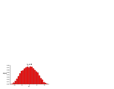
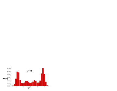
At $l_{p}=5$, the distribution is close to a Gaussian, as seen in Fig. 6. With increasing values of $l_{p}$ the distribution becomes significantly non-Gaussian (Fig. 7) and ultimately evolves to a bimodal distribution resembling two Gaussians(Fig. 8). The distributions are reminiscent of a first order transition, except for the fact that for $l_{p}\simeq W$, the distributions clearly show four peaks as evident in Fig. 7.

Figure 7: Distribution function $P(\Psi)$ for $l_{p}=15$. There are 4 peaks and a valley at $\Psi=0$, and this is no longer described by a Gaussian.

Figure 8: Distribution function $P(\Psi)$ for $l_{p}=25$.

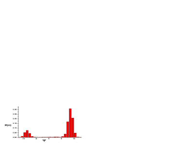
Typical configurations corresponding to the outer peaks are similar to the plot in Fig. 9; spiral in a box. A typical configuration for an inner peak is illustrated in Fig. 10 and shows an elliptical character. In a circular box, the inner peaks are still evident but they do not have the elliptical character (Fig. 10). These peaks are, therefore, more robust than the elliptical shape. Since the only other length scale in the problem, besides, $l_{p}$ and $W$ is the contour length or, equivalently, $R_{g}$, we have future plans of exploring the distributions as a function of $R_{g}$ in order to better understand this intermediate state.

Interactions of a semiflexible polymer with hard (or semisoft) boundaries are known to introduce orientational correlations E.Katzav et al. (2006); Sakaue (2007); Chen et al. (2005); Chen (2007). One example is the transition to liquid crystalline phases of polymers confined between two hard walls Chen et al. (2005) when the persistence length is comparable to the dimensions of the confinement. The shape changes that we are observing in our study have a similar physical origin.

Figure 9: A configuration in the square box corresponding to the outer peak in Fig. 7.

Figure 10: $(a)$ A configuration in a square box corresponding to the inner peak in Fig.7. $(b)$ Same as $(a)$ but in a circular box.

IV Tangent-tangent correlations and effective persistent length in confinement

¿From the discussion above, it is clear that the shape, characterized by the average tangent vector, depends on the relation between $l_{p}$ and $W$. The tangent-tangent correlation function, $C(s,s^{\prime})$, defined as

$$C(s,s^{\prime})\equiv\langle(\mathbb{u}(s)-\langle\mathbb{u}(s)\rangle)\cdot(\mathbb{u}(s^{\prime})-\langle\mathbb{u}(s^{\prime})\rangle)\rangle$$ (5)

is expected to depend on the shape of the polymer. Such changes have been observed in experiments. For example, in actin filaments trapped in narrow channels, $C(s,s^{\prime})$ exhibits a oscillatory behavior, and an effective persistence length, deduced from the correlation function, shows changes from the bare persistence length Köster et al. (2007); Odijk (1983). Because of translational invariance and the indistinguishability of two ends of a polymer chain, $C(s,s^{\prime})$ is only a function of $|s-s^{\prime}|$, and in the simulations, we measure $C(s)\equiv C(s,0)$. Figs. 11, and 12 show $C(s)$ measured at $l_{p}\leq 5$ and $8\leq l_{p}\leq 18$, respectively.

Figure 11: $C(s)$ (Eq.5) for $l_{p}\leq 5$. When $l_{p}<5$, $C(s)$ decays exponentially and then fluctuates around 0; a behavior that is similar to an unconfined chain. When $l_{p}=5$, $C(s)$ begins to show the oscillatory structure. The meansured persistence length $l_{e}\sim l_{p}$.

Figure 12: C(s) (Eq.5) for $8\leq l_{p}\leq 18$. Graphs are labelled by the value of$l_{p}$. In contrast to the behavior observed at small values of $l_{p}$ (11), there is a distinct periodic behavior.

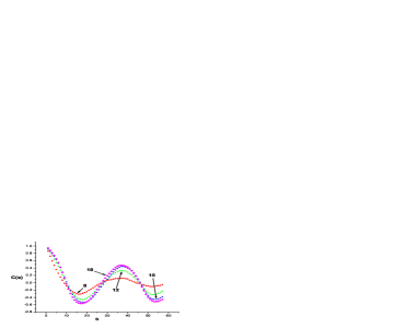
For $l_{p}<5$, $C(s)$ exhibits exponential decay with a length scale which is indistinguishable from the bare persistence length, $l_{p}$. In this regime, where $l_{p}$ is much smaller than $W$, the free energy of the polymer is dominated by the entropy , and the fluctuations resemble those of an unconfined semiflexible polymer.

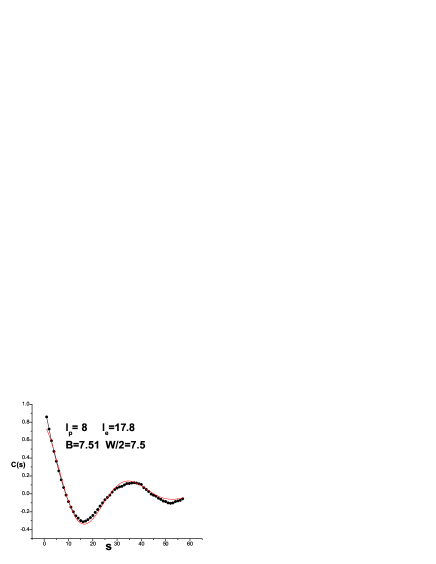
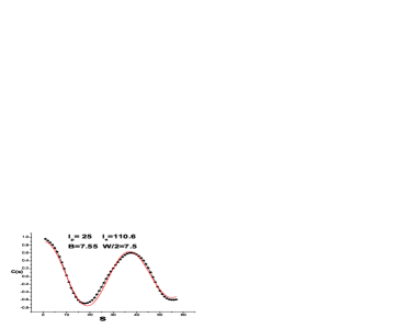
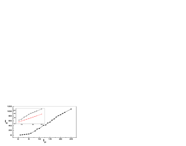
The situation changes for $l_{p}$ larger than or comparable to $W$. As seen from Fig. 12, $C(s)$ exhibits an oscillatory character. A negative value of $C(s)$ indicates a reflection in orientation of the tangent vector. The oscillations, therefore, reflect the constraints imposed on $C(s)$ by the geometry of the confinement and we expect the periodicity to be related to the size of the box, $W$. We therefore represent $C(s)$ as $Ae^{-\frac{s}{l_{e}}}\cos\frac{s}{B}$, with A,B and $l_{e}$ as fitting parameters. From Fig. 13 and 14, we see that this form captures the properties of $C(s)$. In the regime $l_{p}\geq 8$, the parameter $B$ is not sensitive to $l_{p}$ and approaches the value 7.5, which is equal to $W/2$. We can extract the effective persistence length, $l_{e}$, from the fits. The variation of this length, which characterizes the rigidity of the polymer under confinement is shown in Fig. 15. It is clear that $l_{e}$ begins to deviate from $l_{p}$ for $l_{p}\gtrsim 8$. This is the regime in which the distribution of the order parameter $\Psi$ starts exhibiting multiple peaks but the average order parameter is still close to zero.

Figure 13: Fit of C(s) by the function $Ae^{-\frac{s}{l_{e}}}\cos\frac{s}{B}$ for $l_{p}=8$. Box size $W=15$, and $B\simeq\frac{W}{2}$.

Figure 14: Fit of C(s) by the function $Ae^{-\frac{s}{l_{e}}}\cos\frac{s}{B}$ for $l_{p}=25$.$l_{e}$ changes and $B\simeq\frac{W}{2}$.

Figure 15: Plot of the effective persistence length $l_{e}$ versus the bare persistence length $l_{p}$ for $W=15$, $L=60$. In the inset, the black dots represent $l_{e}$ vs. $l_{p}$ for $l_{p}\geq 13$ and the red triangles represent the plot of the function (20).

V Gaussian theory of $C(s)$

To understand the origin of the changes in $C(s)$ with the evolving shape of the polymer, we construct a Gaussian model of the fluctuations of the tangent vector. In this model (Fig. 16), the polymer fluctuates around a circle with radius $d$, and the magnitude of the fluctuation $\phi(s)$ is assumed to be small. To describe the energetics of the fluctuations $\phi(s)$, the bending energy term of the Hamiltonian for a worm-like chain is augmented by a harmonic confinement potential $H_{I}$, that penalizes deviations from the circle: $H_{I}=\frac{\lambda}{2}\int_{0}^{L}\phi^{2}(s)\,ds$. The harmonic potential mimics the confinement effects and the parameter, $\lambda$, is an effective coupling constant. This type of modeling has been successfully applied to analyze a polymer confined in a tube Köster et al. (2007); Wagner et al. (2007). The total Hamiltonian is:

$$H=\frac{\kappa}{2}\int_{0}^{L}\bigl{[}\frac{d\mathbb{u}(s)}{ds}\bigr{]}^{2}\,ds+\frac{\lambda}{2}\int_{0}^{L}\phi^{2}(s)\,ds$$ (6)

Figure 16: Mean field model for calculating tangent-tangent correlation function.

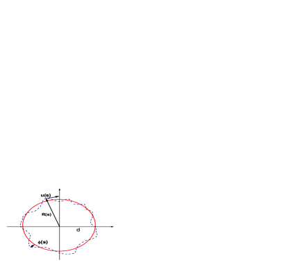
Introducing two unit vectors, $\mathbb{e}_{\theta}(s)$ and $\mathbb{e}_{\rho}(s)$,

$$\mathbb{e}_{\theta}(s)=(-sin\frac{s}{d},cos\frac{s}{d})$$ (7)

$$\mathbb{e}_{\rho}(s)=(cos\frac{s}{d},sin\frac{s}{d})$$ (8)

the tangent vector can be expressed as

$$\mathbb{u}(s)=(1+\frac{1}{d}\phi(s))\mathbb{e}_{\theta}(s)+\frac{d\phi(s)}{ds}\mathbb{e}_{\rho}(s)$$ (9)

Then the Hamiltonian $H$ takes the following form

$$H=\frac{\kappa L}{2d^{2}}+\int_{0}^{L}[(\frac{\kappa}{2d^{2}}+\frac{\lambda d^{2}}{2})\psi^{2}(s)+3\kappa(\frac{d\psi(s)}{ds})^{2}~{},$$ (10)

where $\psi(s)=\frac{\phi(s)}{d}$, the first term represents the bending energy of a circle and the integral represents the energy from the fluctuations. Here we make use of $\int_{0}^{L}\psi(s)\,ds=0$ since the length of the polymer is fixed. In addition, we have retained only the leading order gradients of $\psi$ in the harmonic potential part in order to be consistent with the terms in the WLC model. The Green’s function is defined as $G(s)=\langle\psi(s)\cdot\psi(0)\rangle$.

In the limit of $L\rightarrow\infty$ , we can decompose the fluctuations into Fourier modes,

$$\psi(s)=\int_{-\infty}^{\infty}{e^{iqs}\psi(q)}\,dq$$ (11)

and obtain an expression for $H$ and $G(s,s^{\prime})$ in the Fourier space,respectively.

$$H=\frac{\kappa L}{2d^{2}}+\frac{L}{2\pi}\int_{0}^{\infty}[(\frac{\kappa}{2d^{2}}+\frac{\lambda d^{2}}{2})+3\kappa q^{2}]|\psi(q)|^{2}\,dq$$ (12)

$$G(q)=\frac{2\pi}{L}\frac{1}{(\frac{\kappa}{2d^{2}}+\frac{\lambda d^{2}}{2})+3\kappa q^{2}}$$ (13)

The Green’s in real space is then given by $G(s)\propto e^{-s/l_{e}}$, where the length $l_{e}$ is:

$$l_{e}=(\frac{6\kappa}{\frac{\kappa}{d^{2}}+\lambda d^{2}})^{\frac{1}{2}}$$ (14)

The correlation function $C(s)$ is related to $G(s)$ by

$$C(s)=\cos\frac{|s|}{d}(1-d^{2}\frac{\partial^{2}}{\partial{s}^{2}})G(s)$$

$$+2d\sin\frac{|s|}{d}\frac{\partial{G(s)}}{\partial{s}}$$ (15)

Using the form of $G(s)$, we obtain:

$$C(s)=e^{-s/l_{e}}(\cos\frac{|s|}{d}-2\frac{d}{l_{e}}\sin\frac{|s|}{d}-\frac{d^{2}}{l_{e}^{2}}\cos\frac{|s|}{d})$$ (16)

In the limit of small $\frac{d}{l_{e}}$ , the leading contribution to $C(s)$ is $e^{-\frac{s}{l_{e}}}\cos\frac{s}{d}$, a form that is in remarkably good agreement with the simulation results shown in Figs 13, 14, for which the condition $d<<l_{e}$ is satisfied. The radius $d$ of the circle can be obtained by minimizing the mean-field free energyStrey et al. (1999), $F$, corresponding to the Hamiltonian $H$:

$$e^{-F}=\int{\cal{D}}[\psi(q)]e^{-\frac{\kappa L}{2d^{2}}-\frac{L}{2\pi}\int_{-\infty}^{\infty}[3\kappa q^{2}+(\frac{\kappa}{2d^{2}}+\frac{\lambda d^{2}}{2})]|\psi(q)|^{2}\,dq}$$ (17)

Integrating out the Gaussian functional, leads to:

$$F=\frac{\kappa L}{2d^{2}}+\frac{L}{2\pi}\int_{0}^{\infty}\ln(3\kappa q^{2}+\frac{\kappa}{2d^{2}}+\frac{\lambda d^{2}}{2})\,dq$$ (18)

Setting $\frac{\partial F}{\partial d}=0$, yields

$$\frac{12\kappa^{2}}{\lambda d^{4}-\kappa}=\sqrt{\frac{6\kappa}{\frac{k}{d^{2}}+\lambda d^{2}}}$$ (19)

The effective coupling constant $\lambda$ was introduced to mimic the effects of the confining box. Making use of the observation that $d=\frac{W}{2}$ in the simulations, we can determine $\lambda$ in terms of $W$ and $\kappa$. Using this result, we subsequently obtain $l_{e}$ in terms of $l_{p}$ and $W$:

$$l_{e}=\frac{\sqrt{3}}{2}\sqrt{W^{2}+6l_{p}^{2}+2\sqrt{3}l_{p}\sqrt{3l_{p}^{2}+W^{2}}}$$ (20)

With increasing values $l_{p}$, $l_{e}$ is predicted to increase linearly with $l_{p}$ for $l_{p}\gg\frac{W}{\sqrt{6}}$. Comparing to the results of simulations (Fig.15), it its seen that the predictions of the Gaussian theory are in semi quantitative agreement with the simulations for $l_{p}\geq 13$. This linear dependence is different from the stiff polymer confined in the tube, for which $l_{e}\propto l_{p}^{\frac{1}{3}}$ Odijk (1983); Köster et al. (2007).

VI Summary

We have investigated the conformational and elastic properties of a single semiflexible polymer confined in 2D square box using numerical simulations based on a widely used lattice model of polymers, the BFM. Since effects of the competition among configurational entropy, bending energy and excluded volume are included, this simplified model leads to non-trivial results. By mapping the polymer configurations onto the tangent space, we visualized changes in conformation of the polymer as the bending rigidity was increased from a disordered shape to an intermediate elliptical shape and eventually to a spiral shape (Fig. 3, 4). We introduced an order parameter (Eq. 4) to characterize the shapes and the distribution of the order parameter provided further insight into the nature of the shape changes. We used a meanfield approach to calculate the tangent-tangent correlation function and the effective persistence length.

The combination of numerical and analytical results provides a detailed picture of the conformational and elastic properties of a polymer under extreme confinement. The variation of the persistence length with confinement has been studied previously under tube confinement where the polymer is unconstrained in one dimension. Our results make specific predictions about the more extreme form of confinement where the polymer is constrained in all dimensions. The definition of the order parameter, introduced to characterize shapes in two dimensions, can be easily generalized to higher dimensions and should prove useful for characterizing shapes of polymers under confinement.

VII ACKNOWLEDGMENT

We acknowledge many useful discussions with Josh Kalb, Michael Hagan and Jane Kondev. This work was supported in part by NSF-DMR-0403997.

References

- J.Kindt et al. (2001) J.Kindt, S.Tzlil, A. Ben-Shaul, and W.Gelbart, PNAS 98, 13671 (2001).
- Odijk (2004) T. Odijk, Phil. Trans. R. Soc. Lond. A 362, 1497 (2004).
- Ali et al. (2004) I. Ali, D. Marenduzzo, and J. Yeomans, J. Chem. Phys. 121, 8635 (2004).
- Jiang et al. (2006) W. Jiang, J. Chang, J. Jakana, J. K. P. Weigele, and W. Chiu, Nature 439, 612 (2006).
- E.Katzav et al. (2006) E.Katzav, M.Adda-Bedia, and A.Boudaoud, PNAS 103, 18900 (2006).
- Köster et al. (2007) S. Köster, D. Steinhauser, and T. Pfohl, J. Phy.: Condens. Matter 17, S4091 (2007).
- G.Morrison and Thirumalai (2005) G.Morrison and D. Thirumalai, J. Chem. Phys. 122, 194907 (2005).
- Muthukumar (2001) M. Muthukumar, Phys. Rev. Lett. 86, 3188 (2001).
- A. Arnold and et al (2007) D. F. A. Arnold, B. Bozorgui and S. J. et al, J. Chem. Phys. 127, 164903 (2007).
- Matysiak et al. (2006) S. Matysiak, A. Montesi, M. Pasquali, A. Kolomeisky, and C. Clementi, Phys. Rev. Lett. 96, 118103 (2006).
- Slonkina and Kolomeisky (2003) E. Slonkina and A. Kolomeisky, J. Chem. Phys. 118, 7112 (2003).
- Sakaue and Raphaël (2006) T. Sakaue and E. Raphaël, Macromolecules 39, 2621 (2006).
- Carmesin and Kremer (1988) I. Carmesin and K. Kremer, Macromolecules 21, 2819 (1988).
- Moukhtar et al. (2007) J. Moukhtar, E. Fontaine, C. Faivre-Moskalenko, and A. Arneodo, Phys. Rev. Lett. 98, 178101 (2007).
- Baschnagel and Binder (1995) J. Baschnagel and K. Binder, Macromolecules 28, 6808 (1995).
- Yamakawa (1971) H. Yamakawa, Modern Theory of Polymer Solutions (Harper and Row, New York, 1971).
- Wilhelm and Frey (1996) J. Wilhelm and E. Frey, Phys. Rev. Lett. 77, 2581 (1996).
- Liu and Chakraborty (2006) Y. Liu and B. Chakraborty (2006), unpublished.
- Doi and Edwards (1986) M. Doi and S. Edwards, The Theory of Polymer Dynamics (Oxford, 1986).
- Valle et al. (2005) F. Valle, M. Favre, P. Rios, A. Rosa, and G. Dietler, Phys. Rev. Lett. 95, 158105 (2005).
- Chen (2007) J. Chen, Phys. Rev. Lett. 98, 088302 (2007).
- Chen et al. (2005) J. Chen, D. Sullivan, and X. Yuan, Europhys. Lett. 72, 89 (2005).
- Dubrovin et al. (1992) B. Dubrovin, A. Fomenko, and S. Novikov, Modern Geometry-Methods and Applications Part I (Springer-Verlag, 1992).
- Sakaue (2007) T. Sakaue, Macromolecules 40, 5206 (2007).
- Odijk (1983) T. Odijk, Macromolecules 16, 1340 (1983).
- Wagner et al. (2007) F. Wagner, G. Lattanzi, and E. Frey, Phys. Rev. E 75, 050902 (2007).
- Strey et al. (1999) H. H. Strey, V. A. Parsegian, and R. Podgornik, Phys. Rev. E 59, 999 (1999).