The galaxy luminosity function of the Abell 496 cluster and its spatial variations

Abstract

Context. The faint-end slopes of galaxy luminosity functions (LFs) in clusters of galaxies have been observed in some cases to vary with clustercentric distance and should be influenced by physical processes (mergers, tides) affecting cluster galaxies. However, there is a wide disagreement on the values of the faint-end LF slopes, ranging from $-1$ to $-2.3$ in the magnitude range $-18<M_{r}<-14$.

Aims. We investigate the LF in the very relaxed cluster Abell 496.

Methods. Our analysis is based on deep images obtained at CFHT with MegaPrime/MegaCam in four bands ($u^{*}$$g^{\prime}$$r^{\prime}$$i^{\prime}$) covering a 1$\times$1 deg² region, which is centered on the cluster Abell 496 and extends to near its virial radius. The LFs are estimated by statistically subtracting a reference field taken as the mean of the 4 Deep fields of the CFHTLS survey. Background contamination is minimized by cutting out galaxies redder than the observed Red Sequence in the $g^{\prime}-i^{\prime}$ versus $i^{\prime}$ colour-magnitude diagram.

Results. In Abell 496, the global LFs show a faint-end slope of $-1.55\pm 0.06$ and vary little with observing band. Without colour cuts, the LFs are much noisier but not significantly steeper. The faint-end slopes show a statistically significant steepening from $\alpha=-1.4\pm 0.1$ in the central region (extending to half a virial radius) to $-1.8\pm 0.1$ in the Southern envelope of the cluster. Cosmic variance and uncertain star-galaxy separation are our main limiting factors in measuring the faint-end of the LFs. The large-scale environment of Abell 496, probed with the fairly complete 6dFGS catalogue, shows a statistically significant 36 Mpc long filament at $\rm PA=137^{\circ}$, but we do not find an enhanced LF along this axis.

Conclusions. Our LFs do not display the large number of dwarf galaxies ($\alpha\approx-2$) inferred by several authors, whose analyses may suffer from field contamination caused by inexistent or inadequate colour cuts. Alternatively, different clusters may have different faint-end slopes, but this is hard to reconcile with the wide range of slopes found for given clusters and for wide sets of clusters.

1 Introduction

Clusters of galaxies represent an extreme environment for galaxy evolution, either in situ or through the accretion of galaxies within groups, which are situated in the filamentary network of our hierarchical Universe.

The analysis of the galaxy luminosity function (LF) in several wavebands is a good way to sample the history of the faint galaxy population (e.g. Adami et al. 2007) including star formation history, evolutionary processes and environmental effects. In particular, the slope of the faint-end of the LF is a direct indicator of the importance of dwarf galaxies, which are expected to be more fragile in the environment of clusters.

The great majority of studies of the LF indicate faint-end slopes in the range $-0.9$ to $-1.5$, but these mostly did not reach very faint magnitudes (see Table 1 in De Propris et al. 2003 and references therein). Recent deep imaging has shed more light on the LF at faint luminosities. Table 3 shows deep (fainter than absolute magnitude $M=-16$) estimations of the faint-end slope: most studies conclude to fairly shallow slopes $\alpha\simeq-1.3$ (with typical uncertainties of 0.1 to 0.2), while several point to faint-end slopes as steep as $\alpha\approx-2.3$, which diverges in luminosity (unless the LF becomes shallower or is cut off at some very faint luminosity).

Part of the wide range of faint-end slopes may be caused by cosmic variance of the background counts. The range of faint-end slopes of the LF may also be due to different mass buildup histories of clusters, through spherical and filamentary infall and major cluster-cluster mergers. However, some of this dispersion in slopes could be caused by systematic uncertainties such as in the star/galaxy separation or through different surface brightness cuts.

Spectroscopic-based LFs would alleviate this problem, but until recently, such spectroscopic-based LFs do not extend fainter than $M=-16$. The exceptions are studies by Rines & Geller (2007) and Mamon et al. (2008) who both find shallow slopes for Virgo cluster galaxies down to $M_{r}=-14$, as well as Penny & Conselice (2007) for the Perseus cluster core.

Unfortunately, galaxy formation simulations do not yet probe the galaxy LF down to sufficiently faint luminosities: the deepest study, by Lanzoni et al. (2005), probed the LF with the GALICS semi-analytical galaxy formation model only down to $M_{B}<-16.5$ (they found $\alpha\simeq-1.3$ in the $B$ band and $\simeq-1.4$ in the $K$ band within the virial radii of clusters, and $\alpha\simeq-1.0$ between 1 and typically 3 virial radii).

The present paper aims at clarifying the debate on the faint-end of the LF and on understanding the different effects of spherical and filamentary infall on the LF. Indeed, the influence of infall on the galaxy population, in particular on the LF is not always well understood, except for a few clusters, such as Coma (e.g. Adami et al. 2007). To achieve this aim, we chose to analyse the very relaxed cluster, Abell 496, known to be very regular both at X-ray and optical wavelengths, and also from a dynamical point of view (Durret et al. 2000). Our data cover a field of view that is wide enough to reach the virial radius and thus probe a variety of environments. The LFs are computed after a better filtering of artefacts through a minimum galaxy width, a better filtering of background galaxies through the rejection of galaxies redder than the Red Sequence of early-type galaxies, and make use of a thorough analysis of the uncertainties due to cosmic variance, photometric errors and imperfect star/galaxy separation. Our general motivation is to obtain LFs in various regions of Abell 496 and compare them with previous works.

The paper is organised as follows. We present our MegaCam data and data reduction in Section 2. In Section 3, we describe how we compute LFs using large comparison fields from the CFHTLS to statistically subtract the fore- and background galaxy population. In Section 4, we present our results obtained for the LFs of Abell 496 in various regions. In Section 5, we briefly discuss our results concerning the LFs in terms of large scale environmental effects on the cluster galaxy populations. Finally, in Section 6 we compare our LFs to other determinations of the Abell 496 LF, and we discuss the discrepancy between our moderate faint-end slope and the steep faint-end slopes recently found by several authors in several clusters.

With a mean heliocentric velocity of $9885\,\rm km\,s^{-1}$ (Durret et al. 2000), Abell 496 has a (luminosity) distance modulus of 35.73, and the scale is 0.636 kpc arcsec^-1 (including cosmological corrections). We give magnitudes in the AB system.

2 Observations and data reduction

2.1 MegaCam cluster data

Abell 496 is centered at J2000 equatorial coordinates $04^{h}33^{m}37.1^{s},-13^{\circ}14^{\prime}46^{\prime\prime}$. It has an angular virial radius of $0.77^{\circ}$ (virial radius of 1.9 Mpc), obtained by extrapolating the radius of overdensity 500 (Markevitch et al. 1999, measured relative to the critical density of the Universe) to the radius of overdensity 100.

The MegaCam field covers an area corresponding to 2.3$\times$2.3 Mpc² at the cluster redshift. We centered our images of Abell 496 on the cluster centre (i.e. on the cD galaxy). This means that we can cover the whole Abell 496 area and its immediate infalling layers within the virial radius.

Abell 496 was observed at CFHT with the large field MegaPrime/MegaCam camera in November 2003 on program 03BF12, P.I. Cayatte (see Table 1). Images were reduced by the TERAPIX pipeline using the standard reduction tool configuration. We refer the reader to http://terapix.iap.fr/ for reduction details.

Table 1: Observation characteristics

Name	Useful area	Exp. time					PSF				Obs.
	(deg2)	(sec)					(FWHM in arcsec)				Date
		$u^{*}$	$g^{\prime}$	$r^{\prime}$	$i^{\prime}$		$u^{*}$	$g^{\prime}$	$r^{\prime}$	$i^{\prime}$
Abell 496	0.82	$13\,680$	$7\,820$	$3\,780$	$3\,570$		1.13	1.06	0.88	0.94	11/2003
Deep 1	0.77	38 946	24 893	60 854	134 863		1.06	0.96	0.92	0.91	$<$09/2006
Deep 2	0.79	5 281	16 655	31 988	72 734		0.89	0.96	0.90	0.91	$<$09/2006
Deep 3	0.83	19 146	21 392	59 574	109 049		1.15	0.96	0.94	0.89	$<$09/2006
Deep 4	0.82	50 867	24 262	72 736	140 981		1.03	0.98	0.88	0.87	$<$09/2006
W1	—–	2 215	2 436	1 179	4 189		$1.04\pm 0.09$	$0.96\pm 0.05$	$0.86\pm 0.11$	$0.85\pm 0.12$	$<$09/2006

Note: The W1 values are means over the 19 Wide subfields of the Wide field.

Object extraction was made using the SExtractor package (Bertin & Arnouts 1996) in the double-image mode. The CFHTLS pipeline at the TERAPIX data centre creates a $\chi^{2}$ image based upon the quadratic sum of the images in the different wavebands. Objects are then detected on this image. In contrast with the CFHTLS images, our set of $u^{*}$$g^{\prime}$$r^{\prime}$$i^{\prime}$ images for each of the two clusters presents important differences in their PSFs (see Table 1). For this reason, we chose a different approach from that of the TERAPIX data centre: instead of using the $\chi^{2}$ image as the reference image, we use the band with the best seeing in our data: $r^{\prime}$. Detections were performed in this band and object characteristics were measured in all bands. The detections and measures were made using the CFHTLS parameters, among which an absolute detection threshold of 0.4 ADU above the background ($\mu<27.34$ in all bands), a minimal detection area of 3 pixels and a 7$\times$7 pixel gaussian convolution filter of 3 pixels of FWHM. In each of the $u^{*}$, $g^{\prime}$, $r^{\prime}$ and $i^{\prime}$ output catalogues, we only kept objects with semi-minor axes larger than 1 pixel and mean surface brightness within the half-light radius greater than $\mu=26.25$ in order to remove artefacts.

We measured Kron magnitudes (MAG_AUTO in SExtractor), with the default SExtractor settings. We used the photometric calibration given by the TERAPIX data processing centre. Since the fluxes in different bands are measured within the same Kron elliptical aperture, we derive colours by simply subtracting the magnitudes. Therefore, our colours are not affected by aperture effects and are only slightly affected by the differences in the PSF between the two bands involved.

Using simulations, we also estimate the completeness levels and reliabilities of our detections (see e.g. Driver et al. 1998b). This is crucial, since we intend to compare our data with CFHTLS data that were not observed exactly in the same conditions. For this, we used the SkyMaker package (Bertin & Fouqué 2007) to build images with the same noise and point spread function as our MegaCam images on the one hand and CFHTLS Deep images on the other hand. The objects fed into SkyMaker were either spherical to flattened Sérsic bulges or thin exponential disks. The Sérsic shape and effective radius are specified functions of luminosity that Mamon & Łokas (2005) obtained from the luminous galaxies of Abell 496 and Coma data of Márquez et al. (2000), while for the dwarfs we considered the relations given by Binggeli & Jerjen (1998). The central $B$-band disk surface magnitudes were extrapolated from a gaussian distribution $\mu_{B}(0)=21.5\pm 1$. The fraction of ellipticals is 60% in clusters and null in the field. The galaxy luminosity function was taken from Popesso et al. (2006) for the cluster and from Blanton et al. (2003) for the field.

Completeness (ratio of real detections to real sources) and reliability (ratio of real to total detections) were then measured by cross-correlation between the SkyMaker input and the SExtractor output catalogue. We found that up to $i^{\prime}$=23, for both kinds of images, SExtractor finds 80% of the objects, and among the detected objects, only 10% are artefacts.

We then performed a star-galaxy separation. Instead of using the neural-network star-galaxy classification method of SExtractor, we placed the detections in a diagram of size (i.e. the half light radius) versus magnitude in the band with the best seeing. The variation of the PSF over the images has been corrected for using a technique similar to that of McCracken et al. (2003). Stars are the smallest objects and are located in a well defined strip up to $r^{\prime}$$\approx$21, thus allowing the separation. At fainter magnitudes, stars and galaxies overlap and individual classification is no longer possible. For magnitudes range where the half light radius distribution is bimodal, we perform a statistical star/galaxy separation, assuming gaussian distributions of $\log r_{50}$ for both stars and galaxies, in different magnitude bins. This is illustrated in Fig. 1 for the fairly faint magnitude bin $21<r^{\prime}<21.5$.

Figure 1: Distribution of half-light radii in the magnitude bin $22<r^{\prime}<22.5$. The vertical line shows the star/galaxy separation deduced from the Besançon model.

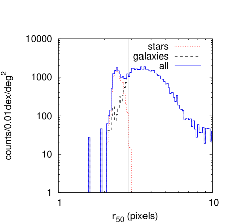
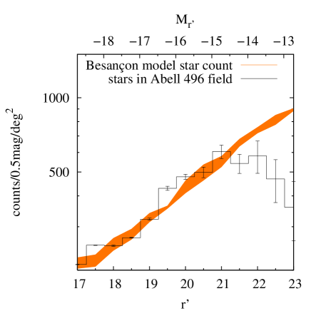
Fig. 2 compares our star counts with those from the Besançon model (Robin et al. 2003). We ran the Besançon model six times in order to get the error on these counts. We did the same with our algorithm. At bright magnitudes ($r^{\prime}<21$), the two distributions coincide. However, at faint magnitudes ($r^{\prime}>21$), our star counts decrease, while the Besançon model counts keep increasing. This could be due to a steeper fall of the stellar density distribution in the direction of Abell 496, in comparison with what is in the Besançon model. Alternatively, we may be wrongly classifying stars as galaxies at $r^{\prime}>21$, and at $r^{\prime}=22$ we may be overestimating the galaxy counts in the Abell 496 field. If we adopt the star counts from the Besançon model, we would end up with 114, 156 and 343 fewer galaxies at $r^{\prime}$ = 21.5, 22.0 and 22.5, respectively. However, if there were as many stars as predicted by the Besançon model, then, for $22<r^{\prime}<22.5$ (see Fig. 1), the distribution of stellar half light radii would rise to a maximum (near $r_{50}=1.3$ pixels) fall to a minimum (near 1.6 pixels), then rise again (to the limit of 1.8 pixels). It is difficult to understand what would cause this final rise. Therefore, in what follows, we adopt our own estimation of the star counts.

We also corrected magnitudes for Galactic extinction based on the Schlegel, Finkbeiner, & Davis (1998) maps. We finally computed the useful covered area (cf. Table 1), by masking all saturated stars, spikes and CCD edges. Galaxies and stars brighter than $r^{\prime}=18$ occupy less than 2% of the pixels of our image.

Figure 2: Comparison of star counts obtained with the Besançon model (Robin et al. 2003) (orange shaded region) and from the Abell 496 image (black solid histogram) using our star-galaxy separation.

The final catalogue will be electronically available at the following address: http://www.cencos.fr/ and in a few months the images will be available at the same address.

2.2 CFHTLS comparison field data

We used the CFHTLS Deep (D1, D2, D3 and D4, i.e. 4 MegaCam fields) and Wide (W1, W2 and W3, 59 MegaCam fields) as comparison field data. Because the LFs are computed by subtraction of the average of the 4 Deep fields (DFs) from the Abell 496 field, objects were re-extracted from the 4 DFs in exactly the same manner as in the cluster field: i.e., with the same detection waveband ($r^{\prime}$ rather than $\chi^{2}$ images) the same SExtractor parameters (including the same 0.4 ADU threshold, which given the same zero point corresponds to the same absolute threshold), and the 1 pixel minimum semi-minor axis. Since the Deep images are deeper than the Abell 496 images, we apply the same cut of mean surface magnitude within the half-light radius of $\mu<26.25$ for all 4 wavebands.

We chose the DFs as reference fields (rather than the CFHTLS Wide fields) because their greater depth ensures smaller photometric errors in our range of magnitudes than those of the Wide fields. Moreover, the DFs were selected to be free of rich nearby structures, which is not the case for the Wide CFHTLS fields, which are shallower (except in $i^{\prime}$) than the Abell 496 field.

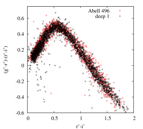
We checked that the cluster and reference fields have compatible photometric calibration. For this we made a colour-colour diagram, shown in Fig. 3, in which we corrected the magnitudes for galactic extinction using the Schlegel et al. (1998) model, and shifted the D1 $i^{\prime}$ magnitudes by +0.02 to force a match.

Figure 3: Colour-colour diagram for $17<r^{\prime}<20$ stars in the A496 (open red circles) and D1 (black crosses) fields, corrected for extinction, and with a shift of the D1 $i^{\prime}$ photometry by +0.02 magnitude.

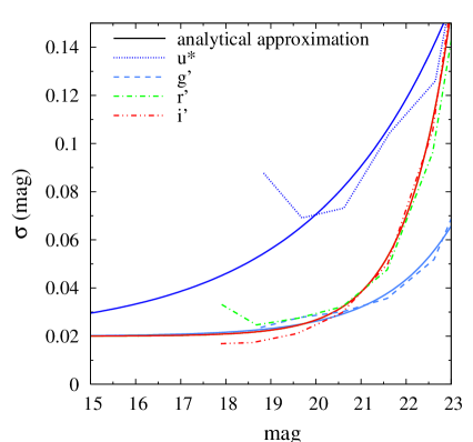
The W1 region (19 MegaCam fields) of the CFHTLS was considered to estimate the magnitude uncertainties as a function of magnitude in an external way. For this, we considered the overlapping areas of the 19 W1 fields. In these areas, we compiled the objects observed twice, and this allowed to estimate the magnitude difference as a function of magnitude in the $u^{*}$, $g^{\prime}$, $r^{\prime}$ and $i^{\prime}$ bands. We only selected objects located more than 400 pixels away from the field edges in order to avoid artificially increasing the magnitude uncertainties due to border effects. These uncertainties are shown in Fig. 4.

We used the TERAPIX object catalogues for the W1 fields, for which detections were done on the $\chi^{2}$ images. In each waveband, the W1 fields have the same measurement threshold as the Abell 496 image. However, the measurement isophote is noisier in the W1 fields (except in the $i^{\prime}$ band). but with the same area on average. Therefore, the W1 magnitude uncertainties should be upper limits for the Abell 496 magnitude uncertainties.

These uncertainties can be approximated by

$$\sigma_{m}=0.02+\alpha\exp\left[\frac{m-m_{1}}{\delta_{m}}\right]\ ,$$ (1)

where $(\alpha,m_{1},\delta_{m})$ = (1.2, 29.5, 3.0), (2.5, 29.0, 1.5), (1.0, 25.0, 1.0) and (1.0, 25.0, 1.0) for $u^{*}g^{\prime}r^{\prime}i^{\prime}$ respectively. These expressions are used to compute the uncertainties on galaxy counts. Note that although the W1 pointings had comparable PSFs to the Abell 496 PSFs, the integration times were smaller, except in the $i^{\prime}$ band (see Table 1). Hence, the photometric errors derived from the W1 field are upper limits in the $u^{*}$, $g^{\prime}$ and $r^{\prime}$ bands.

Figure 4: Magnitude uncertainties estimated from overlapping areas in the 19 CFHTLS W1 fields (dotted and dashed curves) with their analytical approximation (eq. [1], solid curves ).

We also recomputed the area coverage for the Deep and Wide fields from the CFHTLS mask files (see Table 1).

3 Description of the methods

3.1 Luminosity function calculations

The basic method is to statistically estimate the fore- and background contributions to the cluster lines of sight using comparison fields free of rich nearby structures (Oemler 1974).

We compute the LF in the standard fashion: we subtract the reference field counts (the mean of the 4 DFs) from the cluster field counts. The uncertainty is estimated as follows. In a first step, we compute the uncertainties coming from errors on magnitude measurements: starting from a catalogue of magnitudes $\{m_{i}\}$, we create mock catalogues $\{m^{\prime}_{i}\}$, where $m^{\prime}_{i}$ are gaussian distributed random variables of mean $m_{i}$ and standard deviation $\sigma(m_{i})$ estimated from overlapping areas in the 19 CFHTLS W1 fields (cf. Fig. 4). Uncertainties on distributions are then $\sigma_{m}=\sigma\{N(m^{\prime})\}$. In a second step, we compute the uncertainties due to the cosmic variance using the 59 CFHTLS Wide fields:

$$\sigma_{\rm CV}^{2}(m)=\sigma^{2}\{N_{\rm Wide}(m)\}-\langle\sigma_{m}^{2}(m)\rangle_{\rm Wide}\ ,$$ (2)

where $\langle\rangle_{\rm Wide}$ means the median over the 59 Wide fields. It should be stressed that $\sigma_{\rm CV}(m)$ defined in this way implicitly takes into account the statistical uncertainties on the star-galaxy separation (cf. Fig. 2). Finally, we add quadratically all uncertainties:

$$\sigma^{2}\{N^{\rm Cl}(m)\} = \sigma_{m}^{2}\{N^{\rm Cl}_{\rm los}(m)\}+\sigma_{\rm CV}^{2}(m)$$ (3)

$$+\,\frac{1}{4}\left[\sigma_{m}^{2}\{N^{\rm DF}(m)\}+\sigma_{\rm CV}^{2}(m)\right]\ ,$$

where $N^{\rm Cl}$, $N^{\rm Cl}_{\rm los}$ and $N^{\rm DF}$ are the counts from the cluster, the cluster field and the mean of the 4 DFs, respectively. The factor of 4 corresponds to the 4 DFs. All these uncertainties are plotted in Fig. 5 for Abell 496 in the $r^{\prime}$ band.

Figure 5: Uncertainties on the global LF of Abell 496 in the $r^{\prime}$ band for all galaxies, i.e. without selection from the colour-magnitude diagram. For comparison, we show the Poisson error calculated on the gross counts of Abell 496. Note that we defined cosmic variance (eq. [2]) with the Poisson contribution.

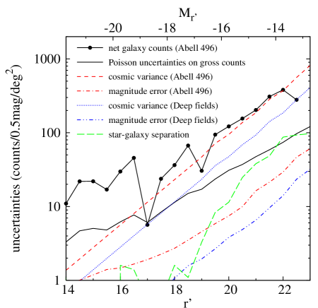
The uncertainty in the galaxy counts given in equation (3) as well as the contribution of star/galaxy separation to the uncertainty in the counts shown in Fig. 5 are purely statistical. One should also consider systematic contributions to this uncertainty, in particular those from star/galaxy separation. Indeed, the difference in galaxy counts after subtraction of the stars either from our star counts or from the Besançon model is almost as large as the cosmic variance of the galaxy counts of the Abell 496 cluster field. However, our analysis of Sect. 2.1 suggests that this systematic uncertainty is smaller than the difference between our estimated star counts and those obtained with the Besançon model.

3.2 Improvement using colour magnitude relations

LFs computed directly from the method described above show very big error bars mainly due to the cosmic variance (cf. Fig. 5). This problem has already been highlighted (e.g. Oemler 1974; Durret et al. 2002). We improve our analysis by removing those objects whose colour imply that they are background objects. We considered $g^{\prime}-i^{\prime}$ because it corresponds to the highest quality magnitude wavebands.

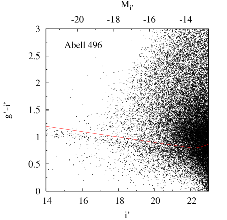
Fig. 6 shows the colour magnitude relations of Abell 496, where no background subtraction has been made. We see a well defined Red Sequence that decreases linearly with $i^{\prime}$, down to at least $M_{i}=-14.5$, as

$$(g^{\prime}-i^{\prime})_{\rm RS}\simeq 1.75-0.05\,i^{\prime}\ ,$$ (4)

consistent with what has been known since Bower et al. (1992). We assume that this Red Sequence is real and corresponds to the reddest galaxies of the cluster. We therefore select only galaxies slightly (0.15 magnitude) above our Red Sequence. Because our photometric errors increase with magnitude, the strict application of this colour cut would lead to an incompleteness at the faint-end. Therefore we use the cut

$$g^{\prime}\!-\!i^{\prime} \!\leq\! (g^{\prime}\!-\!i^{\prime})_{\rm RS}+\hbox{Max}\left(0.15,1.5\,\sigma_{g^{\prime}\!-\!i^{\prime}}\right)$$ (5)

$$\!=\! 1.75-0.05\,i^{\prime}$$

$$\qquad+\hbox{Max}\!\left[0.15,1.5\,\sqrt{\sigma_{g}^{2}\left(0.95\,i\!+\!1.75\right)+\sigma_{i}^{2}(i)}\right]\ ,$$

where we wrote $\sigma^{2}_{g^{\prime}-i^{\prime}}=\sigma_{g^{\prime}}^{2}+\sigma_{i^{\prime}}^{2}$, used the Red Sequence (eq. [4]) to translate $g^{\prime}$ to $i^{\prime}$, and took $\sigma_{g}(g^{\prime})$ and $\sigma_{i}(i^{\prime})$ from equation (1). The factor 1.5 in the first equality of equation (5) ensures that we are 93% complete (assuming a gaussian probability distribution function, hereafter pdf).

The colour cut of equation (5) is represented in Fig. 6 by the red curve. While our colour cut may lead to a loss of atypically red cluster galaxies (e.g. dusty objects), we are confident that such a population, if it exists, is small, and will only marginally decrease our completeness. On the other hand, the colour cut will drastically improve our reliability in the net cluster counts (indeed, our tests have shown that without the colour cuts, the LF is much noisier). Hereafter, all LFs as well as the cosmic variance are computed using this selection.

Figure 6: $i^{\prime}/g^{\prime}-i^{\prime}$ colour-magnitude diagram for Abell 496. The red curve shows the upper limit of galaxy selection to compute the LFs.

4 Results

We computed LFs both for the whole field of view and for 16 subfields. The subfields define a regular square grid of 15$\times$15 arcmin² each and allow a good compromise between spatial resolution and uncertainties in individual magnitude bins. We used 1 magnitude bins to limit the uncertainties. Several subregions are then defined including a certain number of subfields with common properties; they were chosen without assuming circular symmetry for the cluster.

Figure 7: Global luminosity functions for Abell 496 in the four bands with the best fits (in red).

Table 2: Faint-end slopes of Abell 496

Region	$20\leq u^{*}\leq 23$	$18\leq g^{\prime}\leq 22$	$17\leq r^{\prime}\leq 22$	$17\leq i^{\prime}\leq 22$
	$-15.73\leq M_{u^{*}}\leq-12.73$	$-17.73\leq M_{g^{\prime}}\leq-13.73$	$-18.73\leq M_{r^{\prime}}\leq-13.73$	$-18.73\leq M_{i^{\prime}}\leq-13.73$
All	${-1.68\pm 0.35}$	${-1.53\pm 0.08}$	${-1.62\pm 0.05}$	${-1.52\pm 0.05}$
All (no colour cuts)	${-1.78\pm 0.51}$	${-1.61\pm 0.17}$	${-1.73\pm 0.18}$	${-1.58\pm 0.24}$
Centre	${-1.60\pm 0.27}$	${-1.43\pm 0.07}$	${-1.39\pm 0.08}$	${-1.41\pm 0.05}$
South	${-1.87\pm 0.34}$	${-1.89\pm 0.14}$	${-1.79\pm 0.11}$	${-1.80\pm 0.10}$
East-North-West	${-1.88\pm 0.69}$	${-1.48\pm 0.22}$	${-1.40\pm 0.25}$	${-1.58\pm 0.12}$

Note: the magnitude intervals correspond to the centres of 0.5 magnitude bins (All) and 1.0 magnitude bins (Centre, South, East-North-West).

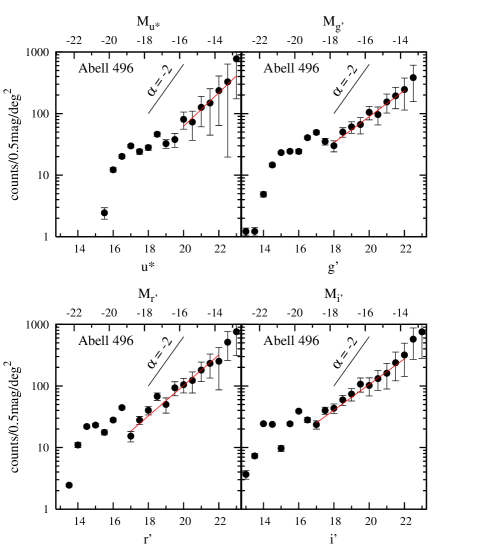
The LFs of Abell 496 in the four bands are displayed in Fig. 7 (the corresponding data are given in Table .2 of the appendix), showing that the shapes of the global LFs of the Abell 496 field are similar in the four bands, with the faint-ends increasing linearly. As these LFs do not look like Schechter functions, we decided to fit only the faint-ends by a power-law. The expression in terms of magnitude is given by:

$$\Phi(M)=10^{-0.4(\alpha+1)(M-M_{0})}.$$

The best fit slopes $\alpha$ of the overall LFs are given in Table 2. We used the Levenberg-Marquardt method (e.g. Press et al. 1992) to fit the data. Error bars were computed from 1000 parametric bootstraps, where the pdf of the net counts is assumed gaussian with a width obtained from the pdf of the gross galaxy counts of the 59 Wide fields. The faint-end slopes vary from band to band, but are typically $\alpha=-1.55\pm 0.05$.

We recomputed the LF in the $r^{\prime}$ band using a much more conservative cut in surface brightness: $\mu_{r}<24.25$ (instead of 26.25). The faint-end slope becomes $\alpha=-1.60\pm 0.05$ (instead of $-1.62\pm 0.05$). Hence, the faint-end slopes appear robust to different cuts in surface brightness.

Had we adopted instead the star counts from the Besançon model (see Fig. 2), the slope of the LF in the $i^{\prime}$ band for the global field would have been $-1.27\pm 0.04$.

We also computed the LFs for galaxies in the Red Sequence (where the redder limit is taken from eq. [5], while the bluer limit is the symmetrical cut, with respective to the average Red Sequence given in eq. [4]). The slopes for the Red Sequence galaxies matched those of the global LFs in all bands. The LFs for galaxies bluer than the Red Sequence are not significantly different but with larger error bars ($\alpha\approx-1.65\pm 0.15$).

Figure 8: Local luminosity functions for Abell 496 in the $r^{\prime}$ band. Each subfield is 15$\times$15 arcmin². X-ray intensity contours with logarithmic steps from ROSAT/PSPC data are superimposed. Three main areas are defined in blue, red and green, which correspond respectively to the centre, the well populated Southern rectangle and the sparse Northern ring.

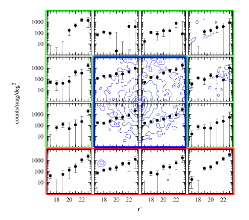
The local $r^{\prime}$ LFs in the 16 subfields of Abell 496 are displayed in Fig. 8. This figure shows that the LFs are not similar over the whole cluster field: subfields in the North, East and West extremities of the cluster are sometimes poorly populated and exhibit large error bars, while subfields in the Southern region show rising LFs. We can thus divide the cluster into three main regions: a central region 30$\times$30 arcmin² (1.15$\times$1.15 Mpc², in blue in Fig. 8), an East-North-West region around this central zone (in green in Fig. 8) and a Southern region (in red in Fig. 8). The central region extends to roughly one half of the virial radius and corresponds to the densest region of the cluster.

Figure 9: Luminosity functions for Abell 496 in the four bands and in the three main areas defined Fig. 8. The blue colour corresponds to the central region, red is for the South and green for the upper East-North-West zone.

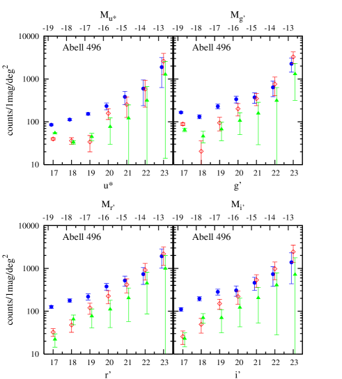
Fig. 9 shows the LFs computed in these three subregions, in the four photometric bands (the corresponding data are given in Table .2 of the appendix). The LFs have faint-end slopes (see Table 2) that are significantly shallower in the centre than in the Southern periphery in all bands except $u^{*}$. The Southern region has a surface density of faint galaxies ($M_{r^{\prime}}>-14$) that is higher than or comparable to that of the central region. If this is not caused by field contamination (see Sect. 6.3), then one would conclude that the faint ($M_{r^{\prime}}>-14$) galaxies do not trace the cluster, which presents no surface density enhancement.

Although they are both contained within the virial radius of the cluster, the two external regions present LFs differing from one another. The Southern region (red) is still quite populated compared to the green region, which is sometimes quite poor with LFs often not significantly positive. Since there are no clusters or groups known nearby (as searched with NED, see Fig. 10), this suggests there may be matter in the Southern region infalling from the surrounding cosmological web, as discussed in the next Section.

5 Large scale filament in the neighbourhood Abell 496

Figure 10: Large scale structure surrounding Abell 496, in a region of 17$\times$17 deg² (41$\times$41 Mpc²), in a redshift slice within $\pm 0.005$ of that of the cluster. The galaxies are taken from 6dFGS-DR3 (points), limited to the completeness limit of $K_{s}<12.65$, which corresponds to $L^{*}/4$ (using the $K_{s}$ field LF of Jones et al. 2006). We also show groups (blue triangles) and clusters (large blue circles) found in NED in the same redshift interval (with their redshifts highlighted). The surrounded red circle shows the position of the cluster centre.

Abell 496 has been shown to be a noticeably quiescent and relaxed cluster (e.g. Durret et al. 2000). The only sign of substructure found was an enhanced concentration of emission line galaxies in the North-West. From Fig. 8, we also see that the Southern part of the surrounding area around the cluster shows a significant galaxy population, with an LF that resembles that of the central cluster.

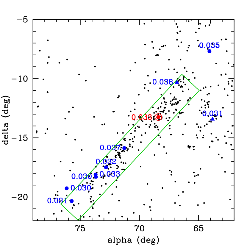
We searched the Six degree Field Galaxy Survey (6dFGS-DR3) database (Jones et al. 2004, 2005, 2008) for nearby galaxies in the large-scale neighbourhood of Abell 496, in a $\pm$0.005 redshift slice around the mean value of 0.033. This slice corresponds to $\pm$1.5 times the velocity dispersion of a massive cluster (1000 km/s), or expressed in terms of physical distance to a slice of 45 Mpc at the redshift of Abell 496. On the plane of the sky, we limited our search to a box of 17$\times$17 deg² (40 Mpc at the cluster redshift). This size is typical of the largest cosmic bubbles (Hoyle & Vogeley 2004).

Fig. 10 shows that the 6dFGS galaxies in the neighbourhood of Abell 496 are more concentrated along a strip in the South-East/North-West direction. This is confirmed by the distribution of groups and clusters that we found in NED (which is much less homogeneous) using the same search criteria. Note that the 6dFGS-DR3 is complete to $K_{s}\leq 12.65$ (Jones et al. 2008) down to galactic latitude $|b|>10^{\circ}$, and in our zone, we have $b<-24^{\circ}$. The galaxies displayed in Fig. 10 are clearly distributed along a large-scale filament, which appears to be at least 30 Mpc long.

We tested the prominence of this filament in the following manner. We searched for the rectangle of length $15^{\circ}$ (36 Mpc at the distance of Abell 496) and width $2^{\circ}$ encompassing the largest amount of points, imposing that Abell 496 lies along the long axis of the rectangle, within $4^{\circ}$ from the closest edge along that axis. We found that the furthest edge along the long axis is at position angle (PA) $137^{\circ}$ anti-clockwise from North. We then built 1000 random samples of as many (487) galaxies in the frame of Fig. 10 as observed, and checked for the most populated rectangle, defined as above, covering 360 PAs in steps of $1^{\circ}$. While the filament in the observed data set has 221 galaxies within the rectangle, none of the 1000 random datasets ever reached more than 81 galaxies. Therefore, the filament at position angle $137^{\circ}$ is highly significant. This filament should constitute a preferential avenue for infalling material into Abell 496, as well as backsplashing material from the cluster. However, this filament does not fully explain the excess of galaxies in the Southern region of Abell 496 since it is inclined relatively to the North-South direction.

6 Discussion and conclusions

6.1 Comparison with previous analyses of Abell 496

The LF of Abell 496 was previously measured by Molinari et al. (1998), who analyzed the cluster in 4 small fields, one including the cluster centre, and by Durret et al. (2002), who measured th LF in a $42^{\prime}\times 28^{\prime}$ field in the $I$ band. The faint-end slopes of $-1.69\pm 0.04$ in $r$ and $-1.49\pm 0.04$ in $i$ found by Molinari et al. are consistent with our slopes of $-1.62\pm 0.05$ and $-1.52\pm 0.05$ in these bands. Moreover, their faint-end slope of $-1.34\pm 0.04$ in $g$ is probably consistent with our slope ($-1.53\pm 0.08$), given that their estimated error neglects cosmic variance, which, as we show in Fig. 5, is many times greater than the Poisson variance. Durret et al. (2002) find a slope of $-1.79\pm 0.01$ in $I$, whereas we find here a slope of $-1.52\pm 0.05$. Given our analysis of cosmic variance, we estimate the error from cosmic variance on the slope of Durret et al. (2002) to be roughly 0.08. If this error estimate is correct, then the difference is faint-end slopes would be statistically significant. This difference may be caused by the different regions probed in the two studies and the different reference fields used.

6.2 Comparison of radial trends with other clusters

Our $g^{\prime}$, $r^{\prime}$ and $i^{\prime}$ LFs exhibit slopes that increase significantly from the centre outwards (Table 2). This agrees with the trend for flatter LFs around cluster cDs found by Lobo et al. (1997), with the steeper slope in the outer envelope of Coma found by Beijersbergen et al. (2002), and with the greater dwarf-to-giant ratio found by Driver et al. (1998a). Note, however, that all three trends are either qualitative or of marginal statistical significance. Although our radial trend is opposite to that found by De Propris et al. (2003) in 2dFGRS clusters, their shallower slope in the cluster envelopes is not statistically significant.

6.3 A ubiquitous dwarf population?

Whereas our faint-end slope for the core of Abell 496 is fairly shallow ($\alpha\simeq-1.4$), it is still steeper than most estimates of the field LF: Blanton et al. (2003) find $\alpha_{r}=-1.05\pm 0.01$ for the SDSS galaxies, while Jones et al. (2006) find $\alpha$ between $-1.10\pm 0.04$ ($J$-band) and $-1.21\pm 0.04$ ($r$-band) for 6dFGS galaxies. However, Blanton et al. (2005) estimate that a careful inclusion of SDSS low surface brightness galaxies yields $\alpha_{r}<-1.3$ and perhaps as steep as $-1.5$. But several authors found very steep slopes ($\alpha$ as steep as $-2.2$) for faint galaxy populations in clusters (see Table 3), suggesting an important population of dwarf galaxies in clusters, which is not seen in the field LFs.

It is difficult to understand how dwarf galaxies could survive better in the hostile cluster environment than in the field. Direct galaxy mergers should have little effect on dwarfs, whose cross-sections are small. Mergers of dwarfs after orbital decay by dynamical friction into the central cD cannot be an explanation: the decay times are expected to be proportional to galaxy mass, so the giant galaxies can disappear into the central cD. However, the orbital decay times for the low mass galaxies should be long enough that the faint-end mass function in clusters would be the same as the field, not steeper. Moreover, there is no observational evidence for luminosity segregation of faint galaxies in clusters (e.g., Pracy et al. 2005). Finally, tidal effects from the cluster potential are the same, to first order, on giant and dwarf galaxies. Given the trend that low luminosity ellipticals are less concentrated than more luminous ones (Graham et al. 2001), the latter will survive better the strong tides near the cluster centre, which should make the LF shallower, not steeper. The only possible explanation for a steeper faint-end slope in clusters would be that galaxies of moderately low luminosity are tidally fragmented by the cluster potential or by close encounters.

Now, if the field counts in the cluster field are underestimated (because the reference fields are slightly underdense), the resultant net cluster counts will be highly contaminated by field counts. Writing the field counts as $dN/dm=\hbox{dex}[\beta\,(m-m_{0})]$ and the cluster faint-end luminosity function as $\Phi(L)\propto L^{\alpha}$, it is easy to show that if the field dominates the net cluster counts, one will end up measuring $\alpha=(-\beta/0.4)-1$. For example, if $\beta=3/5$ (Euclidean counts), one would measure $\alpha=-5/2$, while if $\beta\simeq 0.36$ (as in the DFs in the magnitude range where we are measuring the faint-end slope of the LF), one should find $\alpha=-1.9$.

We are confident that we suffer little from a background contamination of our LFs. Indeed, the faint-end slopes that we have computed for the global LF (Table 2) and for the central region of Abell 496 (Table 2) are all considerably and significantly shallower than $\alpha=-1.9$ (except in the less sensitive $u^{*}$ band). We also took great care not to underestimate the counts in our field count process by the use of very homogeneous field data covering a large enough field of view in order to treat properly the cosmic variance (as described above). Finally the selection in colour that we have applied eliminates (both in the cluster fields and in the fields used for statistical subtraction) very red objects that are very unlikely to belong to the cluster, so the field subtraction is quite conservative and therefore secure.

The MegaCam colour redshift diagrams derived by Ilbert et al. (2006) from the VIMOS VLT Deep Survey (VVDS) followup of the CFHTLS DF show that galaxy spectra are shifted to the red to such an extent that, in the redshift range $0.4<z<0.6$, the bulk of field (intrinsically blue spiral) galaxies become redder in $g^{\prime}-r^{\prime}$ than nearby ellipticals, and the same happens in the range $0.5<z<1.2$ for $r^{\prime}-i^{\prime}$ colours. We are therefore probably contaminated by intrinsically blue (spiral) background galaxies with colours almost as red as our Red Sequence at $z<0.4$ or 0.5.

Note that two of the studies concluding to steep faint-end LF slopes (De Propris et al. 1995; Milne et al. 2007) have negative LFs at some magnitudes, which suggests inadequate background subtraction (Fig. 8 shows that 4 of our 12 non-central local LFs also display negative LFs at some intermediate magnitudes, which makes these particular LFs suspicious). Moreover, all steep faint-end slopes were found by authors who made no colour cuts, with the exception of Popesso et al. (2006). These authors estimated the LFs of clusters in the SDSS, using the statistical subtraction method, and found $\alpha\approx-2.2$. The range of absolute magnitudes where Popesso et al. see the rise in the faint-end LF, [$-17.7,-13.7$], corresponds to apparent magnitudes in the range $18.03<m<22.03$, which matches our analyzed range of apparent magnitudes. It is puzzling that we do not find in our deeper images the low surface brightness dwarf population found by Popesso et al. in the SDSS images.

Figure 11: Our $u^{*}-r^{\prime}$ vs $i^{\prime}$ colour-magnitude diagram for Abell 496. The dashed contours are for our selected cluster members using equation (5), while the solid (red) contours (same levels, spaced by factors of 1.6) are the galaxies identified as field galaxies, because they are redder than our Red Sequence of equation (5). Also shown are the limits used by Popesso et al. (2006) to separate their red cluster galaxies and field galaxies (upper horizontal line) and their blue and red cluster galaxies (lower horizontal line), after correcting both for $(u^{*}-r^{\prime})_{\rm MegaCam}=(u-r)_{\rm SDSS}-0.35$, as found using the matches in a field of Abell 85 for which we had both SDSS catalogues and reduced MegaCam images. The vertical lines delimit the region where Popesso et al. clearly found a steep faint-end LF slope.

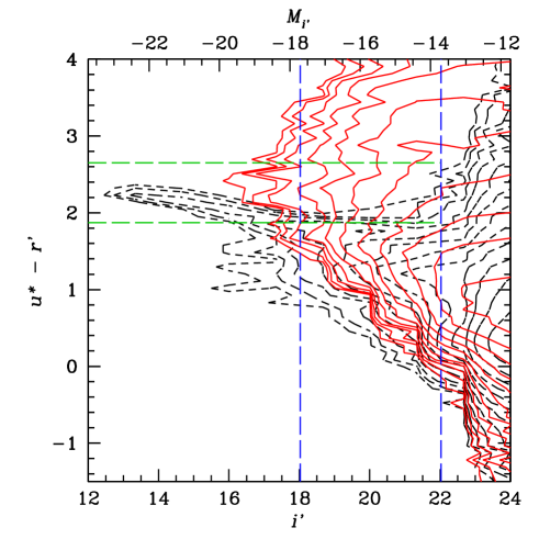
Fig. 11 displays the $u^{*}-r^{\prime}$ vs $i^{\prime}$ colour-magnitude diagram of the Abell 496 field. The Red Sequence is clearly visible at bright magnitudes and its red edge is still sharp at magnitudes $18<i^{\prime}<22$. The galaxies called red cluster members by Popesso et al. and fainter than $M_{i}^{\prime}=-19$ are almost all field galaxies according to our colour-magnitude diagram. Similarly, at $M_{i}^{\prime}=-16.5$, our Red Sequence (or its extrapolation) becomes bluer than the blue-red galaxy cut of Popesso et al.. This suggests that an increasing fraction of both Popesso et al.’s red and blue galaxies are in fact field galaxies.

From inspection of the $u^{*}-g^{\prime}$ and $g^{\prime}-r^{\prime}$ colour-redshift diagrams of Ilbert et al. (2006), one infers that the $u^{*}-r^{\prime}$ colour cut used by Popesso et al. should vary negligibly with redshift. This explains why the galaxies we assign to the field (solid red contours in Fig. 11) — because they are redder than our sharp $g^{\prime}-i^{\prime}$ vs $i^{\prime}$ Red Sequence — pollute the $u^{*}-r^{\prime}$ vs $i^{\prime}$ colour-magnitude diagram. Therefore, colour cuts based upon $u^{*}-r^{\prime}$ are not efficient in rejecting background galaxies (with $z\la 0.4$).

Nevertheless, while LF analyses based upon the statistical subtraction method with inappropriate or inexistent colour cuts should lead to noisier LFs, it is not clear why they should be biased to steeper slopes, unless the noise is such that the faint-end of the LF fluctuates from positive to negative (which is not the case for the global LF of Popesso et al.). Although simulations by Valotto et al. (2001) showed that clusters selected in 2D will have faint-end slopes much steeper than what they put in their simulations ($-1.4$ instead of $-1$ in roughly the same absolute magnitude range as where Popesso et al. found their slope of $-2.3$), Valotto et al. have also shown that LFs measured in clusters selected in 3D, such as all the clusters reported in this paper (including the X-ray selected clusters studied by Popesso et al.), show no bias in the faint-end slope. A confirmation of this result is that X-ray selected clusters show shallower faint-end slopes than do non X-ray clusters (Valotto et al. 2004), which are expected to be more prone to projection effects.

A possible cause for the discrepancy between different analyses could be the uncertainties from star/galaxy separation. This is a serious issue for our analysis, because Abell 496 lies at lower absolute galactic latitude ($b=-36^{\circ}$) than our reference DF fields ($b=-58^{\circ},42^{\circ},60^{\circ}$ and $-53^{\circ}$), so that Abell 496 is more contaminated by stars. Indeed, our $i^{\prime}$-band LF has a considerably shallower faint-end slope of $-1.27\pm 0.04$ instead of $-1.52\pm 0.05$ (Table 2). Moreover, in general, the errors on star/galaxy separation could go either way, leading to either an underestimation or overestimation of the faint-end LF slope.

A possible explanation for the wide range of faint-end slopes (see Table 3) is cosmic variance: some clusters may exhibit steeper slopes than others. However, inspecting the slopes found in the literature (Table 3), one notices a wide range of slopes for the same cluster analyzed in similar wavebands, magnitude ranges and fields of view (contrast the slopes in similar regions of Coma of $-1.7$, $-1.8$ of Lobo et al. 1997 and Trentham 1998a with the slopes shallower or equal to $-1.4$ of Andreon & Cuillandre 2002). Moreover, the two studies that have enough clusters to ‘beat’ cosmic variance have inconsistent slopes ($-2.2$ Popesso et al. 2006 and $-1.4$ Trentham 1998b) in the magnitude range $-18$ to $-14$.

6.4 Conclusions

We have analyzed the galaxy LFs in the relaxed cluster of galaxies Abell 496. We have shown that the LFs are not only well-defined in the central region (with a faint-end slope $\alpha=-1.4\pm 0.1$), but also in the South. A concentration of clusters is indeed observed towards the South-East and along a filament extending South-East to North-West (Fig. 10), suggesting the existence of a cosmological filament linking Abell 496 with various poor clusters and groups. However, such a filament cannot be very dense since no X-ray emission is detected in this direction, contrary to what is observed in Abell 85 (Durret et al. 2003).

We discuss the disagreement of our fairly shallow faint-end slope for Abell 496 with that found by other authors in this and other clusters. Although it is clear that a careful estimate of the reference field galaxy counts and their cosmic variance are crucial, there may also be a cosmic variance in the faint-end slopes of cluster LFs. We find that uncertainties in the star/galaxy separation can be responsible for some (but probably not all) of the scatter in the faint-end LF slopes given in the literature. We highlight the removal of galaxies redder than the Red Sequence as a means to reduce the noise in the LFs, but it is not clear if the lack of adequate colour cuts causes a bias towards steeper slopes. The advent of very deep spectroscopy in cluster fields should rapidly settle the issue of the faint-end slope of the cluster LF.

Table 3: Comparison of deep photometrically-estimated cluster galaxy luminosity functions

Cluster(s)	$r_{\rm max}/r_{100}$	abs. mag range	$\alpha$	Reference
Local Group	3.6	$M_{V}<-9$	–1.1	Pritchet & van den Bergh (1999)
Virgo	1.1	$M_{B}<-13.1$	–1.25	Sandage et al. (1985)
Virgo	1.1	$M_{B}<-11.1$	–1.3	Sandage et al. (1985)
Virgo	$0.24\!\times\!0.24$	$-15.6<M_{R}<-11.1$	–2.26	Phillipps et al. (1998)
Virgo	$2\!\times\!0.4\!\times\!1.2$	$-18<M_{B}<-11$	–1.35	Trentham & Hodgkin (2002)
Virgo	$2\!\times\!0.4\!\times\!1.2$	$-17<M_{B}<-14$	–1.7	Trentham & Hodgkin (2002)
Coma	$0.08\!\times\!0.08$	$M_{R}<-11.6$	–1.42	Bernstein et al. (1995)
Coma	$0.08\!\times\!0.08$	$-11.6<M_{R}<-9.4$	–2.0	Bernstein et al. (1995)
Coma	$0.58\!\times\!0.24$	$M_{V}<-15.5$	–1.8	Lobo et al. (1997)
Coma	$0.3\!\times\!0.3$	$-15.6<M_{B}<-10.6$	–1.7	Trentham (1998a)
Coma	$0.3\!\times\!0.3$	$-17.6<M_{R}<-11.6$	–1.7	Trentham (1998a)
Coma	0.8	$M_{U}<-13.4$	–1.32	Beijersbergen et al. (2002)
Coma	0.8	$M_{B}<-13.4$	–1.37	Beijersbergen et al. (2002)
Coma	0.8	$M_{r}<-13.4$	–1.16	Beijersbergen et al. (2002)
Coma	$0.28\!\times\!0.43$	$M_{B,V,R}<-12.8$	–1.25	Andreon & Cuillandre (2002)
Coma	$0.28\!\times\!0.43$	$M_{V}<-11.3$	–1.4	Andreon & Cuillandre (2002)
Coma	$0.28\!\times\!0.43$	$M_{R}<-11.8$	–1.4	Andreon & Cuillandre (2002)
Coma	$0.6\times 0.6$	$-19.1<M_{R}<-14.6$	–1.55	Iglesias-Páramo et al. (2003)
Coma	0.01	$M_{R}<-9.1$	–2.29	Milne et al. (2007)
Coma	0.01	$M_{R}<-11.3$	–1.9	Adami et al. (2007)
Coma (North)	$0.28\!\times\!0.22$	$M_{B}<-10.5$	–1.48	Adami et al. (2007)
Coma (North)	$0.28\!\times\!0.22$	$M_{R}<-11.3$	–1.74	Adami et al. (2007)
Coma (South)	$0.28\!\times\!0.22$	$M_{B}<-10.5$	–1.32	Adami et al. (2007)
Coma (South)	$0.28\!\times\!0.22$	$M_{R}<-11.3$	–1.28	Adami et al. (2007)
Abell 426	$0.1\times 0.1$	$-19.4<M_{I}<-13.4$	–1.56	De Propris & Pritchet (1998)
Abell 496	$4\!\times\!0.19\!\times\!0.19$	$M_{g}<-13.2$	–1.34	Molinari et al. (1998)
Abell 496	$4\!\times\!0.19\!\times\!0.19$	$M_{r}<-13.2$	–1.69	Molinari et al. (1998)
Abell 496	$4\!\times\!0.19\!\times\!0.19$	$M_{i}<-13.2$	–1.49	Molinari et al. (1998)
Abell 496	$0.9\!\times\!0.6$	$M_{I}^{\rm AB}<-13.7$	–1.79	Durret et al. (2002)
Abell 539	$0.24\times 0.24$	$-18.5<M_{I}<-14.0$	–1.42	De Propris & Pritchet (1998)
Abell 1185	0.9	$M_{B}<-12.4$	–1.25	Andreon et al. (2006)
Abell 1185	0.9	$M_{V}<-13.2$	–1.28	Andreon et al. (2006)
Abell 1185	0.9	$M_{R}<-13.7$	–1.28	Andreon et al. (2006)
Abell 1367	$0.7\times 0.7$	$M_{R}<-14.3$	–1.07	Iglesias-Páramo et al. (2003)
Abell 2199	$0.04\times 0.04$	$M_{B}<-10.5$	–2.16	De Propris et al. (1995)
3 clusters	$0.05\times 0.05$	$M_{I}<-13.0$	–2.28	De Propris et al. (1995)
9 clusters	$0.25\times 0.25$	$-19<M_{B}<-14$	–1.4	Trentham (1998b)
9 clusters	$0.25\times 0.25$	$-14<M_{B}<-11$	–1.8	Trentham (1998b)
Ursa Major	6.8	$-17<M_{R}<-11$	–1.1	Trentham et al. (2001)
69 RASS/SDSS clusters	0.7	$M_{g}<-13.7$	–1.98	Popesso et al. (2006)
69 RASS/SDSS clusters	0.7	$M_{r}<-13.7$	–2.19	Popesso et al. (2006)
69 RASS/SDSS clusters	0.7	$M_{i}<-13.7$	–2.26	Popesso et al. (2006)
69 RASS/SDSS clusters	0.7	$M_{z}<-13.7$	–2.25	Popesso et al. (2006)

Notes: The method used is field subtraction, except for the Local Group study of Pritchet & van den Bergh (1999) and the first line of the Virgo analysis by Sandage, Binggeli, & Tammann (1985), which are based upon raw counts, while the second line of the Virgo analysis of Sandage et al. adds a statistical background correction. The virial radii are from Mamon et al. (2004) (Virgo), Łokas & Mamon (2003) (Coma), this paper (Abell 496), Markevitch et al. (1999) (Abell 2199), and otherwise adapted from the velocity dispersions measured by Fadda et al. (1996), when available (only for 5 out of the 9 clusters of Trentham 1998b and 3 of 4 for De Propris et al. 1995). Magnitude ranges are converted to $H_{0}=72\,\rm km\,s^{-1}\,Mpc^{-1}$. Typical errors on $\alpha$ are in the range 0.1 to 0.2.

Table 4: Luminosity functions for Abell 496 in the whole field (Fig. 7) and in the three main areas (Fig. 9).

mag bin	$u^{*}$		$g^{\prime}$		$r^{\prime}$		$i^{\prime}$
	All
13.5	0$\ \pm\$	0	1$\ \pm\$	0	2$\ \pm\$	0	7$\ \pm\$	1
14	0$\ \pm\$	0	5$\ \pm\$	1	11$\ \pm\$	1	24$\ \pm\$	1
14.5	0$\ \pm\$	0	15$\ \pm\$	1	22$\ \pm\$	1	24$\ \pm\$	1
15	0$\ \pm\$	0	23$\ \pm\$	1	23$\ \pm\$	1	10$\ \pm\$	1
15.5	2$\ \pm\$	1	24$\ \pm\$	1	18$\ \pm\$	1	24$\ \pm\$	1
16	12$\ \pm\$	1	24$\ \pm\$	2	28$\ \pm\$	2	39$\ \pm\$	2
16.5	20$\ \pm\$	2	39$\ \pm\$	3	44$\ \pm\$	3	28$\ \pm\$	3
17	30$\ \pm\$	2	49$\ \pm\$	3	15$\ \pm\$	3	24$\ \pm\$	4
17.5	24$\ \pm\$	2	35$\ \pm\$	4	27$\ \pm\$	4	42$\ \pm\$	5
18	27$\ \pm\$	3	29$\ \pm\$	6	41$\ \pm\$	6	45$\ \pm\$	7
18.5	46$\ \pm\$	3	50$\ \pm\$	9	69$\ \pm\$	9	58$\ \pm\$	11
19	32$\ \pm\$	5	61$\ \pm\$	13	51$\ \pm\$	14	72$\ \pm\$	17
19.5	38$\ \pm\$	9	63$\ \pm\$	20	91$\ \pm\$	24	106$\ \pm\$	28
20	80$\ \pm\$	25	103$\ \pm\$	26	104$\ \pm\$	28	101$\ \pm\$	33
20.5	76$\ \pm\$	36	100$\ \pm\$	31	118$\ \pm\$	46	119$\ \pm\$	47
21	125$\ \pm\$	65	161$\ \pm\$	53	174$\ \pm\$	63	152$\ \pm\$	72
21.5	156$\ \pm\$	104	188$\ \pm\$	73	233$\ \pm\$	98	243$\ \pm\$	117
22	239$\ \pm\$	172	251$\ \pm\$	132	258$\ \pm\$	166	321$\ \pm\$	177
22.5	328$\ \pm\$	308	390$\ \pm\$	228	536$\ \pm\$	257	583$\ \pm\$	304
	Center
17	85$\ \pm\$	4	165$\ \pm\$	7	126$\ \pm\$	9	110$\ \pm\$	11
18	112$\ \pm\$	6	131$\ \pm\$	13	177$\ \pm\$	16	195$\ \pm\$	22
19	153$\ \pm\$	10	229$\ \pm\$	29	218$\ \pm\$	35	283$\ \pm\$	44
20	232$\ \pm\$	42	336$\ \pm\$	61	378$\ \pm\$	67	306$\ \pm\$	82
21	382$\ \pm\$	132	372$\ \pm\$	102	520$\ \pm\$	137	461$\ \pm\$	154
22	594$\ \pm\$	356	637$\ \pm\$	251	733$\ \pm\$	311	734$\ \pm\$	355
23	1895$\ \pm\$	1264	2256$\ \pm\$	813	1922$\ \pm\$	910	1387$\ \pm\$	949
	South
17	39$\ \pm\$	2	88$\ \pm\$	7	32$\ \pm\$	6	25$\ \pm\$	8
18	36$\ \pm\$	6	20$\ \pm\$	15	47$\ \pm\$	15	49$\ \pm\$	18
19	33$\ \pm\$	13	94$\ \pm\$	32	119$\ \pm\$	34	150$\ \pm\$	40
20	157$\ \pm\$	44	201$\ \pm\$	64	225$\ \pm\$	75	221$\ \pm\$	76
21	252$\ \pm\$	126	347$\ \pm\$	109	417$\ \pm\$	150	535$\ \pm\$	174
22	578$\ \pm\$	358	757$\ \pm\$	351	917$\ \pm\$	384	976$\ \pm\$	431
23	2605$\ \pm\$	1337	3275$\ \pm\$	1009	2182$\ \pm\$	991	2444$\ \pm\$	1065
	East-North-West
17	54$\ \pm\$	2	64$\ \pm\$	6	22$\ \pm\$	7	22$\ \pm\$	8
18	33$\ \pm\$	3	46$\ \pm\$	13	64$\ \pm\$	16	70$\ \pm\$	17
19	44$\ \pm\$	8	67$\ \pm\$	30	76$\ \pm\$	36	70$\ \pm\$	38
20	76$\ \pm\$	47	106$\ \pm\$	56	110$\ \pm\$	69	122$\ \pm\$	79
21	121$\ \pm\$	126	157$\ \pm\$	128	202$\ \pm\$	145	204$\ \pm\$	151
22	314$\ \pm\$	347	313$\ \pm\$	316	450$\ \pm\$	363	406$\ \pm\$	378
23	1276$\ \pm\$	1262	1308$\ \pm\$	991	992$\ \pm\$	991	720$\ \pm\$	1038