Effective temperature of active matter

Abstract

We follow the dynamics of an ensemble of interacting self-propelled motorized particles in contact with an equilibrated thermal bath. We find that the fluctuation-dissipation relation allows for the definition of an effective temperature that is compatible with the results obtained using a tracer particle as a thermometer. The effective temperature takes a value which is higher than the temperature of the bath and it is continuously controlled by the motor intensity.

Active matter is driven out of equilibrium by internal or external energy sources. Its constituents absorb energy from their environment or from internal fuel tanks and dissipate it by carrying out internal movements that lead to translational or rotational motion. A typical example can be found in eukariotes, which are cells organized into complex assemblies by internal structures. In these cells many processes involve the cytoskeleton cytoskeleton , the cellular scaffolding, that is formed by a network of long polar filaments interacting through molecular motors. The latter exert stresses which deform the former and regulate the network dynamics. These structures exhibit a rich variety of viscoelastic properties; by rearranging their structure they change from plastic/fluid to elastic/glassy phases and vice versa. Another celebrated example of active matter are self-propelled particle assemblies in bacterial colonies bacteria .

Here, we address the following fundamental question: which thermodynamic concepts, if any, can be applied to active matter? We focus on the definition of an effective temperature, $T_{eff}$, through the comparison of induced and spontaneous dynamic fluctuations Teff . The notion of such a $T_{eff}$ was introduced in the study of (passive) glassy systems, that is to say, macroscopic objects with a sluggish relaxation that takes them to an asymptotic small-entropy production regime which is, though, still far from equilibrium. In these systems $T_{eff}$ is a good thermodynamic concept. It admits a microcanonical-like definition in which only asymptotically dynamically accessible states contribute to the entropy Makse . $T_{eff}$ can be measured by a fine-tuned thermometer, it satisfies a zero-th law in the sense that it takes the same value for all observables evolving in the same time-scale, and heat flows in the direction of negative effective temperature differences Teff . Moreover, it appears in the modification of fluctuation theorems when applied to systems that cannot equilibrate when let freely evolve Zamponi . These features were confirmed with numerical simulations of a variety of realistic glassy models Binder-Kob and a number of groups are testing these ideas experimentally on colloidal suspensions Teff-exp-coll . Theory suggests that the effective temperature should also be well-behaved in weakly driven systems – in a small entropy production regime Teff . This fact was put to the test in gently sheared super-cooled liquids and glasses Ludovic , vibrated granular matter Makse , and moving vortex phases in superconductors Kolton . In biologically inspired problems the relevance of $T_{eff}$ was already stressed in studies of gene networks Wolynes1 and to reveal the active process in hair bundles Julicher and in a simple three-component model system consisting of myosin II, actin filaments, and cross-linkers mizuno . The modification of the rheological behavior in active filament solutions was also interpreted in terms of a non-equilibrium temperature in ziebert07 .

The role played by $T_{eff}$ in the stability of dynamic phases of motorized particle systems was stressed by Shen and Wolynes Wolynes2 with a variational analysis of the master equation of a similar model to the one we study here. In order to investigate the existence and properties of $T_{eff}$ in active matter we study a schematic statistical physical model: a system of $i=1,\dots,N$ massive, interacting and motorized spherical particles confined to a fixed volume, $V$, in $3d$. Spherical particles are indeed too simple for real applications in the context of cytoskeleton studies. In particular, they are allowed to freely move in space, with no bounds to a preexisting cytoskeletal filaments network. This choice is dictated by the need to highlight the effect of the non-equilibrium drive alone, with no additional effects related to a more complex internal structure. Similar behavior is anyhow expected for other geometries of the constituents. Particles are in contact with a thermal environment that is described by a random noise and a viscous drag. Neglecting hydrodynamics effects, the particles’ velocities ${\bf v}_{i}$ thus evolve with the Langevin equation:

$$m_{i}\dot{\bf v}_{i}=-\xi m_{i}{\bf v}_{i}+{\bf f}_{i}^{s}+{\bf f}^{M}_{i}+{\mathbf{\eta}}_{i}\;.$$ (1)

Here, ${\mathbf{\eta}}_{i}$ is a Gaussian white noise representing thermal agitation with zero mean, and correlations $\langle{\bf\eta}_{i}(t){\bf\eta}_{i}(t^{\prime})\rangle=2\xi m_{i}T\delta(t-t^{\prime})$ (we set $k_{B}=1$ henceforth). The term $-\xi m_{i}{\bf v}_{i}$ is the frictional force and $\xi$ the friction coefficient. The overdamped character of the dynamics is taken into account by considering a large value $\xi=10$. The choice of Eq. (1) in place of a position Langevin equation, where the inertia term $m_{i}\dot{\bf v}_{i}$ is dropped, allows for a more stable Verlet-like integration method and a more realistic description of short time dynamics allentildesley .

The systematic mechanical conservative force on particle $i$ due to all others is ${\bf f}^{s}_{i}\equiv\sum_{j=1}^{N}{\bf f}^{s}_{ij}=-\sum_{j=1}^{N}{\bf\nabla}_{i}U(r_{ij})$, with the $2n$-$n$ Lennard-Jones potential Lekk $U(r_{ij})=4\epsilon[\left(\sigma/r_{ij}\right)^{2n}-\left(\sigma/r_{ij}\right)^{n}]$. $r_{ij}$ is the interparticle distance. The short-range repulsion, parametrized by $\sigma$, prevents the overlapping of the particles and it is then a (soft) measure of the particle diameter. The energy parameter, $\epsilon$, describes the depth of the attraction. The mid-range attraction, $r_{Min}=\sigma 2^{-1/n}$, mimics the effective cross-linking by linker proteins between elements in the cytoskeleton. By choosing $n=18$ we get an adhesive soft-sphere potential with $r_{Min}\ll\sigma$ as often used to describe biomolecular assemblies Wolynes2 ; Rosenbaum . This case also presents the additional advantage that the region of the phase diagram where the metastable liquid phase is accessible in equilibrium is particularly extended. Again, we do not expect significant qualitative differences for other choices of $U$.

Finally, motors apply a force ${\bf f}^{M}_{i}$ on each particle following a stochastic process that mimics the realistic chemical process. For simplicity, we use here a time series of isotropic kicks. During $\tau$ steps of the molecular dynamics trajectory independent forces are applied to a fraction of randomly chosen particles. The subset of propelled particles and the directions of the applied forces change at each power stroke of duration $\tau$. The strength of the force exerted on each particle is chosen to be a fraction of the mean mechanical force acting on the equivalent passive system, $\overline{F}=\frac{1}{N}\sum_{j=1}^{N}|{\bf f}_{ij}^{s}|$. The parameters $\tau$ and $\overline{F}$ and the fraction of motorized particles are chosen consistently in order to induce an out-of-equilibrium steady state always remaining in linear-response conditions. We consider here adamant motors Wolynes2 which act in such a way that the direction of the force is chosen at random isotropically: their action is independent of the structural rearrangements they induce. The case of susceptible motors, which slow down when they drive the system uphill in the (free)-energy landscape, will be investigated in future work.

We integrated Eqs. (1) numerically using Ermak’s algorithm ermak78 ; allentildesley . We henceforth use standard Lennard-Jones units: length, energy and time-units are $\sigma$, $\epsilon$ and $(m\sigma^{2}/\epsilon)^{\frac{1}{2}}$, respectively allentildesley . In all our simulations we used 100 independent configurations with 500 particles. We have checked that larger systems have equivalent structural and dynamical behavior.

Figure 1: (Colour online) The static structure factor, $S(Q)$, for a system in equilibrium and driven out of equilibrium by motors with $f^{M}=50\%\overline{F}$.

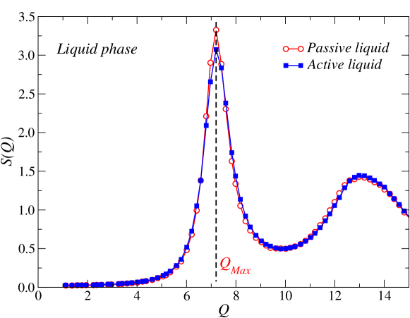
The passive system (motors switched off) is well characterized and presents gas, liquid and crystalline phases depending on the bath temperature and particle density Lekk . By tuning the intensity and direction of the non-conservative forces we drive the system near equilibrium (weak perturbation) or far from equilibrium (strong perturbation). We delay the description of the dynamic phase diagram to a more detailed publication. Here we focus on the driven dynamics of a system at conditions such that it is a liquid in equilibrium: $T=0.8$ and $\rho=1$.

We show data using a time-scale for the power strikes $\tau=5\times 10^{3}$, we apply the force to $10\%$ of the particles and the strength of the non-conservative force, $f^{M}$, is indicated in each figure. Other choices of these parameters give equivalent results. We start by comparing the structure of active and passive matter. In both cases the structure factor, $S(\vec{Q})=\langle\,\rho(\vec{Q},t)\rho^{*}(\vec{Q},t)\,\rangle$, with $\rho(\vec{Q},t)=N^{-1}\sum_{i=1}^{N}e^{i\vec{Q}\vec{r}_{i}(t)}$ the Fourier transform of the instantaneous density, becomes stationary and isotropic after a short transient: $S(\vec{Q},t)\to S(Q)$. In Fig. 1 we show that $S(Q)$ for the passive liquid and the active system with $f^{M}=50\%\overline{F}$ are practically identical, with a maximum located at $Q_{Max}\sim 7.1$ in both cases.

Figure 2: (Colour online) Main panel: the incoherent intermediate scattering function at $Q=Q_{Max}$, for motor force intensities given in the key. Data are shown as a function of simulation time measured in molecular dynamics integration steps (MDs). Inset: the dependence of the $\alpha$ relaxation time on the strength of the motor forces with an exponential fit $\tau_{\alpha}\sim A\exp-(f^{M}/f^{o})$ with $f^{0}\simeq 0.90$.

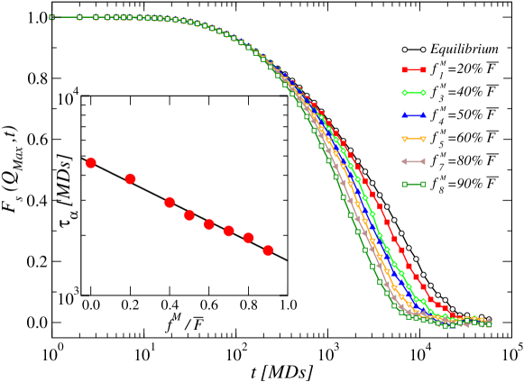
The relaxational dynamics of super-cooled liquids and glasses is usually examined by monitoring the decay of the – possibly two-time dependent – incoherent (one-particle) intermediate scattering function $F_{s}(\vec{Q},t,t_{w})=N^{-1}\sum_{i=1}^{N}\langle\,e^{-i\vec{Q}[\vec{r}_{i}(t+t_{w})-\vec{r}_{i}(t_{w})]}\,\rangle$ Binder-Kob with $t_{w}$ the waiting-time measured after preparation and $t$ the delay time between the total and the waiting times. In the liquid and under the effect of the motors the systems reach an isotropic stationary regime: $F_{s}$ only depends on $Q$ and $t$. Figure 2 displays $F_{s}$ as a function of time-delay in a log-linear scale for several force strengths ranging from zero (equilibrium limit) to $90\%\overline{F}$. The decay is faster for increasing force strengths though remains relatively slow for all drives as demonstrated by the fact that $F_{s}$ decays to zero in a logarithmic time-scale. In the inset we show how the $\alpha$-relaxation time, $\tau_{\alpha}\equiv F_{s}(Q,\tau_{\alpha})=e^{-1}$, decreases for increasing force strength in a linear-log scale, similarly to the shear-thinning phenomenon. The line is $\tau_{\alpha}\sim A\exp-(f^{M}/f^{o})$. At each applied force we find $\tau_{\alpha}\propto Q^{-2}$ (not shown).

Figure 3: (Colour online) Parametric representation of the fluctuation dissipation relation for passive and active matter. The strength of the applied forces are given in the key.

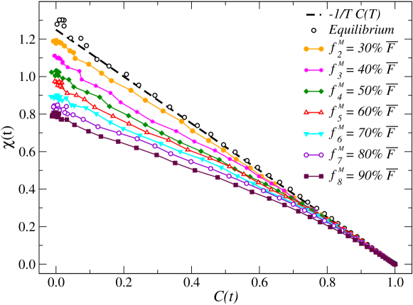
The equilibrium fluctuation-dissipation theorem (FDT) states that the spontaneous fluctuations are related to their associated induced fluctuations by a model-independent formula $T\chi(t,t_{w})=[C(t=0,t_{w})-C(t,t_{w})]$. $C$ is the connected correlation of two observables $O_{1}$ and $O_{2}$, measured at times $t+t_{w}$ and $t_{w}$ respectively. $\chi$ is the linear response of the average of the observable $O_{1}$ measured at time $t+t_{w}$ to an infinitesimal perturbation that modifies the Hamiltonian as $H\to H-hO_{2}$ from $t_{w}$ to $t$: $\chi(t,t_{w})=\langle O_{1}^{h}(t+t_{w})-O_{1}(t+t_{w})\rangle/h$. The choice of the appropriate observables $O_{1}$ and $O_{2}$ follows standard procedures and details about the calculations can be found in Ref. Ludovic . Here, we recall that in interacting particle problems Ludovic it is customary to use $O_{1}(t_{w})=\frac{1}{N}\sum_{i=1}^{N}\epsilon_{i}e^{i\vec{Q}\vec{r}_{i}(t_{w})}$, $O_{2}(t_{w})=2\sum_{i=1}^{N}\epsilon_{i}\cos[\vec{Q}\vec{r}_{i}(t_{w})]$, where the field $\epsilon_{i}=\pm 1$ with probability a half. With this choice, $C(t)=F_{s}(Q,t)$. For each system configuration we averaged over 100 field realizations and considered $Q=Q_{Max}$. In Fig. 3 we show the fluctuation-dissipation relation for passive and active matter. The plots are parametric constructions of the integrated linear response $\chi$ as a function of the correlation function using $t$ as the parameter Teff . In the equilibrium case, FDT holds and minus the inverse slope of $\chi(C)$ is the temperature of the thermal bath, $T=0.8$ in this case. In general, all curves join at $(C=1,\chi=0)$, as imposed by normalization at $t=0$. The ‘initial’ slope is determined by the equilibrium FDT Cudeku . At longer time-differences the curves progressively depart from the equilibrium result to reach other straight lines characterized by slopes that depend on the strength of the motor forces. A time (or correlation) dependent effective temperature is then defined as Teff

$$1/T_{eff}(C)=-d\chi(C)/dC\;.$$ (2)

Interestingly enough, soon after departure from the equilibrium form, the curves approach a new straight line from which one extracts a single value of the effective temperature – within numerical accuracy Houches .

Figure 4: (Colour online) Main panel: probability distribution function of the velocity $v$ of different tracers with masses $m_{tr}$ given in the key. The motor force intensity is $f^{M}=60\%\overline{F}$. The full lines are fits to the Gaussian form (3). Inset: $T_{eff}$ as function of $m_{tr}$ as obtained from the Gaussian fits to the data-points in the main panel.

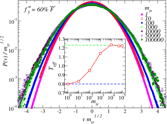
The meaning of $T_{eff}$ as a temperature depends on it verifying a number of conditions expected from such thermodynamic concept. In particular, a temperature should be measurable with a thermometer. A tracer particle with a long internal time-scale (proportional to the square root of its mass) Teff ; Ludovic ; Makse acts as a thermometer that couples to the long time-delay structural rearrangements (and not to the fast vibrations, $t\sim 0$, that yield the ambient temperature, see Fig. 3 and Cudeku ). We then coupled a tracer particle with mass $m_{tr}$ to the active matter via the same Lennard-Jones potential, so that we do not modify the structure factor of the fluid. (The tracer does not couple to the thermal bath.) In Fig. 4 we show the tracers’ velocity distributions (for 10 independent tracers). The data points are superposed to

$$P(v)=\sqrt{\frac{m_{tr}}{2\pi T_{eff}}}\;\exp\left(-\frac{m_{tr}v^{2}}{2T_{eff}}\right)\;,$$ (3)

with $T_{eff}$ the only fitting parameter. The reason why a Maxwellian distribution applies is that the tracer behaves as a normal system immersed in an environment made of active matter. The inset in Fig. 4 displays the dependence of $T_{eff}$ on $m_{tr}$ for one value of the energy pumping force. A very light tracer basically follows the very fast – high frequency – dynamics of its environment and thus measures the bath temperature (lower horizontal dashed line). A heavier tracer feels the slower – low frequency – structural relaxation and measures a higher temperature. A sufficiently heavy tracer only follows the slow dynamics of the sample and therefore measures the actual effective temperature (upper horizontal dashed line), $T_{eff}(f^{M}=60\%\overline{F})\sim 1.23$.

Figure 5: (Colour online) Effective temperature obtained from response-correlation and massive tracer calculations for different motor force intensities.

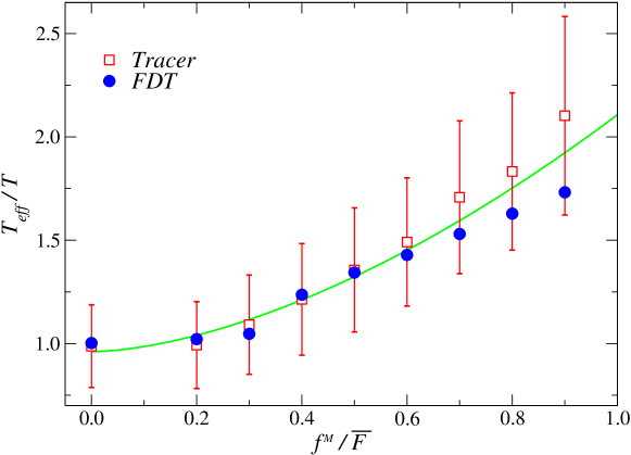
Finally, in Fig. 5 we compare the values of $T_{eff}$ derived from Eqs. (2) and (3). The two measurements yield consistent results, with $T_{eff}$ increasing from $T$ at zero pump to about $2T$ when the strength of the driving forces equals the one of the mechanical forces. We also found that $T_{eff}$ decreases with decreasing $\tau$ (not shown).

Summarizing, we showed that the notion of an effective temperature, defined by studying the deviations from the equilibrium FDT out of equilibrium can be applied to active matter. We demonstrated that the value of the effective temperature measured with a thermometer realized by a tracer particle coincides – within numerical accuracy – with the one obtained from the fluctuation-dissipation relation for all values of the pumping forces. For adamant motors $T_{eff}$ is larger or equal than the bath temperature and increases as a function of the pumping force. This finding is consistent with the intuitive idea that ascribes $T_{eff}$ to the degree of additional agitation caused by the non-conservative forces. It will be interesting to study in detail the case of susceptible motors Wolynes2 which slow down when driving the system uphill in the (free)-energy landscape. It is natural to expect that the effective temperature of such active matter would be lower than the one of the thermal bath. Finally, it is a challenge to derive the above results in the framework of hydrodynamic theories of the kind proposed in hydro .

LFC is a member of Institut Universitaire de France.

References

- (1) B. Alberts, The molecular biology of the cell (Garland, New York, 1994).
- (2) H. C. Berg, Nature 254, 389 (1975); E. Ben-Jacob et al, Phys. Rev. Lett. 75, 2899 (1995).
- (3) L. F. Cugliandolo, J. Kurchan and L. Peliti, Phys. Rev. E 55, 3898 (1997); L. F. Cugliandolo and J. Kurchan, Physica A 263, 242 (1999).
- (4) H. Makse and J. Kurchan, Nature 415, 614 (2002).
- (5) F. Zamponi et al, J. Stat. Mech. (2005) P09013.
- (6) K. Binder and W. Kob, Glassy materials and disordered solids (World Scientific, 2005).
- (7) see, e.g. P. Wang, C. Song, and H. A. Makse, Nature Physics 2, 526 (2006) and refs. therein.
- (8) L. Berthier and J-L Barrat, Phys. Rev. Lett. 89, 95702 (2002); J. Chem. Phys. 116, 6228 (2002).
- (9) A. B. Kolton et al, Phys. Rev. Lett. 89, 227001 (2002).
- (10) T. Lu et al, Biophys. J. 91, 84 (2006).
- (11) P. Martin et al, Proc. Nac. Acad. Sc. USA 98, 14380 (2001).
- (12) D. Mizuno et al, Science 315, 370 (2007).
- (13) F. Ziebert and I. S. Aranson, Phys. Rev. E 76, 1 (2007).
- (14) T. Shen and P. G. Wolynes, Proc. Nac. Acad. Sc. USA 101, 8547 (2004); Phys. Rev. E 72, 041927 (2005).
- (15) M. P. Allen and D. J. Tildesley, Computer simulation of liquids (Clarendon Press, 2nd ed., 1989).
- (16) G. A. Vliegenthart et al, Physica A 263, 378 (1999).
- (17) D. F. Rosenbaum and C. F. Zukoski, J. Cryst. Growth 160, 752 (1996).
- (18) D. L. Ermak and J. A. McCammon, J. Chem. Phys. 69, 1352, 1978.
- (19) L. F. Cugliandolo et al, Phys. Rev. Lett. 79, 2168 (1997).
- (20) For a discussion on the separation of time-scales see L. F. Cugliandolo, in Slow relaxation in glassy systems, J-L Barrat et al eds. (Springer, Berlin, 2003), cond-mat/0210312.
- (21) H. Y. Lee and M. Kardar, Phys. Rev. E 64, 056113 (2001); Y. Hatwalne et al, Phys. Rev. Lett. 92, 118101 (2004); T. B. Liverpool and M. C. Marchetti, Phys. Rev. Lett. 97, 268101 (2006); K. Kruse et al, Phys. Rev. Lett. 92, 078101 (2004)