Fast Estimator of Primordial Non-Gaussianity from Temperature and Polarization Anisotropies in the Cosmic Microwave Background II: Partial Sky Coverage and Inhomogeneous Noise
Abstract
In our recent paper (Yadav et al., 2007) we described a fast cubic (bispectrum) estimator of the amplitude of primordial non-Gaussianity of local type, , from a combined analysis of the Cosmic Microwave Background (CMB) temperature and E-polarization observations. In this paper we generalize the estimator to deal with a partial sky coverage as well as inhomogeneous noise. Our generalized estimator is still computationally efficient, scaling as compared to the scaling of the brute force bispectrum calculation for sky maps with pixels. Upcoming CMB experiments are expected to yield high-sensitivity temperature and E-polarization data. Our generalized estimator will allow us to optimally utilize the combined CMB temperature and E-polarization information from these realistic experiments, and to constrain primordial non-Gaussianity.
1 Introduction
Non-Gaussianity from the simplest inflation models, that are based on a slowly rolling scalar field, is very small (Salopek & Bond, 1990, 1991; Falk et al., 1993; Gangui et al., 1994; Acquaviva et al., 2003; Maldacena, 2003); however, a very large class of more general models, e.g., models with multiple scalar fields, features in inflation potential, non-adiabatic fluctuations, non-canonical kinetic terms, deviations from the Bunch-Davies vacuum, among others, predict substantially higher level of primordial non-Gaussianity (Bartolo et al., 2004, for a review and references therein).
Primordial non-Gaussianity can be described in terms of the 3-point correlation function of Bardeen’s curvature perturbations, , in Fourier space:
| (1) |
Depending on the shape of the 3-point function, i.e., , non-Gaussianity can be broadly classified into two classes (Babich et al., 2004). First, the local, “squeezed,” non-Gaussianity where is large for the configurations in which . Second, the non-local, “equilateral,” non-Gaussianity where is large for the configuration when .
The local form arises from a non-linear relation between inflaton and curvature perturbations (Salopek & Bond, 1990, 1991; Gangui et al., 1994), curvaton models (Lyth et al., 2003), or the New Ekpyrotic models (Koyama et al., 2007; Buchbinder et al., 2007). The equilateral form arises from non-canonical kinetic terms such as the Dirac-Born-Infeld (DBI) action (Alishahiha et al., 2004), the ghost condensation (Arkani-Hamed et al., 2004), or any other single-field models in which the scalar field acquires a low speed of sound (Chen et al., 2007; Cheung et al., 2007). While we focus on the local form in this paper, it is straightforward to repeat our analysis for the equilateral form.
The local form of non-Gaussianity may be parametrized in real space as (Gangui et al., 1994; Verde et al., 2000; Komatsu & Spergel, 2001):
| (2) |
where characterizes the amplitude of primordial non-Gaussianity. Different inflationary models predict different amounts of , starting from to , beyond which values have been excluded by the Cosmic Microwave Background (CMB) bispectrum of WMAP temperature data, , at the level (Komatsu et al., 2003; Creminelli et al., 2006b; Spergel et al., 2006).
So far all the constraints on primordial non-Gaussianity use only temperature information of the CMB. By also having the E-polarization information together with CMB temperature information, one can improve the sensitivity to the primordial fluctuations (Babich & Zaldarriaga, 2004; Yadav & Wandelt, 2005; Yadav et al., 2007). Although the experiments have already started characterizing E-polarization anisotropies (Kovac et al., 2002; Kogut et al., 2003; Page et al., 2007; Montroy et al., 2006), the errors are large in comparison to temperature anisotropy. The upcoming experiments such as Planck satellite will characterize E-polarization anisotropy to a higher accuracy. It is very timely to develop the tools which can optimally utilize the combined CMB temperature and E-polarization information to constrain models of the early universe.
Throughout this paper we use the standard Lambda CDM cosmology with the following cosmological parameters: , , , , , and . For all of our simulations we used HEALPix maps with pixels.
1.1 Generalized Bispectrum Estimator of Primordial Non-Gaussianity
In our recent paper (Yadav et al., 2007) we described a fast cubic (bispectrum) estimator of , using a combined analysis of the temperature and E-polarization observations. The estimator was optimal for homogeneous noise, where optimality was defined by saturation of the Fisher matrix bound.
In this paper we generalize our previous estimator of to deal more optimally with a partial sky coverage and the inhomogeneous noise. The generalization is done in an analogous way to how Creminelli et al. (2006a) generalized the temperature only estimator developed by Komatsu et al. (2005); however, the final result of Creminelli et al. (2006a) (their Eq. (30)) is off by a factor of two, which results in the error in that is much larger than the Fisher matrix prediction, as we shall show below.
The fast bispectrum estimator of from the combined CMB temperature and E-polarization data can be written as , where (Yadav et al., 2007)
| (3) |
| (4) |
| (5) |
| (6) |
| (7) |
| (8) |
and is a fraction of the sky observed. Indices and can either be or . Here, is 1 when , 6 when , and 2 otherwise, is the theoretical bispectrum for (Yadav et al., 2007), is the power spectrum of the primordial curvature perturbations, and is the radiation transfer function of adiabatic perturbations.
It has been shown that the above mentioned estimator is optimal for the full sky coverage and homogeneous noise (Yadav et al., 2007). To be able to deal with the realistic data, the estimator has to be able to deal with the inhomogeneous noise and foreground masks.
The estimator can be generalized to deal with a partial sky coverage and the inhomogeneous noise by adding a linear term to : . For the temperature only case, this has been done in Creminelli et al. (2006a). Following the same argument, we find that the linear term for the combined analysis of CMB temperature and polarization data is given by
| (9) |
where and are the and maps generated from Monte Carlo simulations that contain signal and noise, and denotes the average over the Monte Carlo simulations.
The generalized estimator is given by
| (10) |
which is the main result of this paper. Note that , and this relation also holds for the equilateral shape. Therefore, it is straightforward to find the generalized estimator for the equilateral shape: first, find the cubic estimator of the equilateral shape, , and take the Monte Carlo average, . Let us suppose that contains terms in the form of , where , , and are some filtered maps. Use the Wick’s theorem to re-write the average of a cubic product as . Finally, remove the MC average from single maps, and replace maps in the product with the simulated maps: . This operation gives the correct expression for the linear term, both for the local form and the equilateral form.
One can find the estimator of from the temperature data only by setting . We have compared our formula in the temperature-only limit with the original formula derived by Creminelli et al. (2006a) (their Eq. (30)), and found a discrepancy. To see the discrepancy, let us re-write the estimator as: . Our formula gives , while Eq. (30) of Creminelli et al. (2006a) gives . 111Equation (30) in Creminelli et al. (2006a) is off by a factor of 2. Since we used , to compare our normalization factor with Creminelli et al. (2006a) one needs to divide the normalization in Creminelli et al. (2006a) by a factor of .
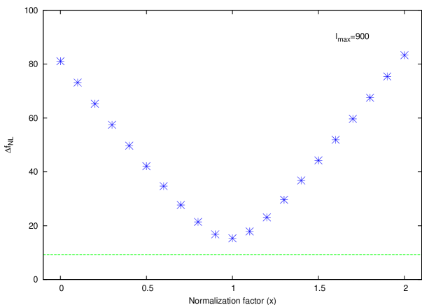
To make sure that our normalization gives the minimum variance estimator, we have done Monte Carlo simulations with varying . We find that minimizes the variance (as shown in Fig. 1). We conclude that the analysis given in Creminelli et al. (2006a) resulted in the larger-than-expected uncertainty in because of this error in their normalization of the linear term.
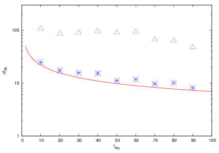
The main contribution to the linear term comes from the inhomogeneous noise and sky cut. For the temperature only case, most of the contribution to the linear term comes from the inhomogeneous noise, and the partial sky coverage does not contribute much to the linear term. This is because the sky-cut induces a monopole contribution outside the mask. In the analysis one subtracts the monopole from outside the mask before measuring , which makes the linear contribution from the mask small (Creminelli et al., 2006a). For a combined analysis of the temperature and polarization maps, however, the linear term does get a significant contribution from a partial sky coverage (see the right panel of Fig. 2). Subtraction of the monopole outside of the mask is of no help for polarization, as the monopole does not exist in the polarization maps by definition. (The lowest relevant multipole for polarization is .)
The estimator is still computationally efficient, taking only (times the sampling, which is of order 100) operations in comparison to the full bispectrum calculation which takes operations. Here refers to the total number of pixels. For Planck, , and so the full bispectrum analysis is not feasible while our analysis is.
2 Results
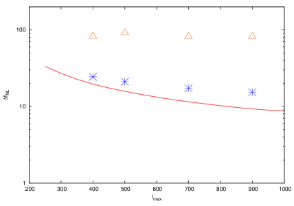
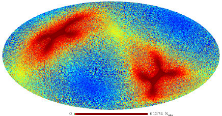
In the left panel of figure 2, we show the variance of using the estimator (with and without the linear term) for the Gaussian CMB simulations in the presence of inhomogeneous noise and partial sky coverage. For this analysis we use the noise properties that are expected for the Planck satellite, assuming the cycloidal scanning strategy (Dupac & Tauber, 2005). Inhomogeneous nature of the noise is depicted in the lower map of figure 4 where we show the number of observations () for the different pixels in the sky. As for the foreground masks, we use WMAP Kp0 intensity mask and P06 polarization mask. We find that, with the inclusion of the linear term, the variance reduces by more than a factor of 5. The linear term greatly reduces the variance approaching the Fisher matrix bound. However, the estimator is close to, but not exactly the same as the Fisher variance prediction in the noise dominated regime.
Nevertheless, we do not observe the increase of variance at higher : the variance becomes smaller as we include more multipoles. This result is in contradiction with the result of Creminelli et al. (2006a) and Creminelli et al. (2006b). We attribute this discrepancy to the error in the normalization of linear term in their formula.
In the right panel of figure 2, we show the variance of again using Gaussian simulations, but now in the presence of flat sky cut and in the absence of any noise. The purpose of the plot is to demonstrate (as pointed out in the previous section) that for the combined CMB temperature and polarization analysis, sky-cut does contribute significantly to the linear term. We find that the generalized estimator does a very good job in reducing the variance excess, and the simulated variance of does accurately saturate the Fisher matrix bound.
Can our estimator recover the correct , i.e., is our estimator unbiased? We have tested our estimator against simulated non-Gaussian CMB temperature and E-polarization maps. The non-Gaussian CMB temperature and E-polarization maps were generated using the method described in Liguori et al. (2007). We find that our estimator is unbiased, i.e., we can recover the value which was used to generate the non-Gaussian CMB maps. The results for the unbiasedness of the estimator are shown in Table 1. The analysis also shows the unbiasedness of the estimator described in Yadav et al. (2007).
| Noise | Sky-cut | |||
|---|---|---|---|---|
| No | flat cut, | |||
| Inhomogeneous | WMAP Kp0 and P06 masks |
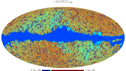
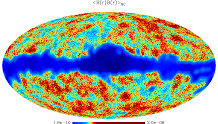
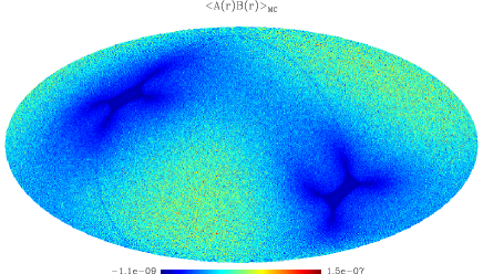
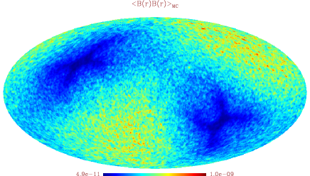
Figures 3 and 4 show the maps and , which appear in the linear term (Eq. 9) of the estimator. These maps are calculated using 100 Monte Carlo simulations of the data. Since the linear term contributes only in the presence of inhomogeneities, we also show these maps calculated with noise-only simulations (i.e. no signal). Notice how these maps correlate with the inhomogeneous noise (as shown in the lower map of figure 4).
3 Conclusion and discussion
Upcoming CMB experiments will provide a wealth of information about the CMB polarization anisotropies together with temperature anisotropies. The combined information from the CMB temperature and polarization data improves the sensitivity to primordial non-Gaussianity (Babich & Zaldarriaga, 2004; Yadav & Wandelt, 2005; Yadav et al., 2007). The promise of learning about the early universe by constraining the amplitude of primordial non-Gaussianity is now well established. In this paper we have generalized the bispectrum estimator of non-Gaussianity described in Yadav et al. (2007), to deal with the inhomogeneous nature of noise and incomplete sky coverage.
The generalization from Yadav et al. (2007) enables us to increase optimality of the estimator significantly, without compromising the computational efficiency of the estimator: the estimator is still computationally efficient, scaling as compared to the scaling of the full bispectrum (Babich & Zaldarriaga, 2004) calculation for sky maps with pixels. For the Planck satellite, this translates into a speed-up by factors of millions, reducing the required computing time from thousands of years to just hours and thus making estimation feasible. The speed of our estimator allows us to study its statistical properties using Monte Carlo simulations.
We have used Gaussian and non-Gaussian simulations to characterize the estimator. We have shown that the generalized fast estimator is able to deal with the partial sky coverage very well and in fact the variance of saturates the Fisher matrix bound. In the presence of both the realistic noise and galactic mask, we find that the generalized estimator greatly reduces the variance in comparison to the Yadav et al. (2007) estimator of non-Gaussianity using combined CMB temperature and polarization data.
Since the estimator is able to deal with the partial sky coverage very effectively, the estimator can also be used to constrain primordial non-Gaussianity using the data from ground and balloon based CMB experiments which observe only a small fraction of the sky. The estimator also solves the problem (Yadav et al., 2007) of non-trivial polarization mode coupling due to foreground masks. Earlier this issue was dealt with by removing the most contaminated modes from the analysis (usually ).
The naive approach of using galactic masks to deal with the polarization contamination is to be refined. Both temperature and polarization foregrounds are expected to produce non-Gaussian signals. Some sources of non-primordial non-Gaussianity are CMB lensing, point sources, and the Sunyaev Zel’dovich effect. Understanding the non-Gaussianity from the polarization foreground sources and refining the estimator to be able to deal with it will be the subject of our future work.
References
- Acquaviva et al. (2003) Acquaviva, V., Bartolo, N., Matarrese, S., & Riotto, A. 2003, Nucl. Phys. B, 667, 119
- Alishahiha et al. (2004) Alishahiha, M., Silverstein, E., & Tong, D. 2004, Phys. Rev. D, 70, 123505
- Arkani-Hamed et al. (2004) Arkani-Hamed, N., Creminelli, P., Mukohyama, S., & Zaldarriaga, M. 2004, Journal of Cosmology and Astro-Particle Physics, 4, 1
- Babich et al. (2004) Babich, D., Creminelli, P., & Zaldarriaga, M. 2004, Journal of Cosmology and Astro-Particle Physics, 8, 9
- Babich & Zaldarriaga (2004) Babich, D. & Zaldarriaga, M. 2004, Phys. Rev. D, 70, 083005
- Bartolo et al. (2004) Bartolo, N., Komatsu, E., Matarrese, S., & Riotto, A. 2004, Phys. Rep., 402, 103
- Buchbinder et al. (2007) Buchbinder, E. I., Khoury, J., & Ovrut, B. A. 2007, Arxiv e-prints, 710
- Chen et al. (2007) Chen, X., Huang, M.-x., Kachru, S., & Shiu, G. 2007, Journal of Cosmology and Astro-Particle Physics, 1, 2
- Cheung et al. (2007) Cheung, C., Creminelli, P., Fitzpatrick, A. L., Kaplan, J., & Senatore, L. 2007, ArXiv:astro-ph/0709.0293
- Creminelli et al. (2006a) Creminelli, P., Nicolis, A., Senatore, L., Tegmark, M., & Zaldarriaga, M. 2006a, Journal of Cosmology and Astro-Particle Physics, 5, 4
- Creminelli et al. (2006b) Creminelli, P., Senatore, L., Zaldarriaga, M., & Tegmark, M. 2006b, ArXiv Astrophysics e-prints, astro-ph/0610600
- Dupac & Tauber (2005) Dupac, X. & Tauber, J. 2005, A&A, 430, 363
- Falk et al. (1993) Falk, T., Rangarajan, R., & Srednicki, M. 1993, ApJ., 403, L1
- Gangui et al. (1994) Gangui, A., Lucchin, F., Matarrese, S., & Mollerach, S. 1994, ApJ., 430, 447
- Górski et al. (2005) Górski, K. M., Hivon, E., Banday, A. J., Wandelt, B. D., Hansen, F. K., Reinecke, M., & Bartelmann, M. 2005, ApJ, 622, 759
- Kogut et al. (2003) Kogut, A., Spergel, D. N., Barnes, C., Bennett, C. L., Halpern, M., Hinshaw, G., Jarosik, N., Limon, M., Meyer, S. S., Page, L., Tucker, G. S., Wollack, E., & Wright, E. L. 2003, ApJS, 148, 161
- Komatsu et al. (2003) Komatsu, E., Kogut, A., Nolta, M. N., Bennett, C. L., Halpern, M., Hinshaw, G., Jarosik, N., Limon, M., Meyer, S. S., Page, L., Spergel, D. N., Tucker, G. S., Verde, L., Wollack, E., & Wright, E. L. 2003, ApJ., 148, 119
- Komatsu & Spergel (2001) Komatsu, E. N. & Spergel, D. N. 2001, Phys. Rev. D, 63, 063002
- Komatsu et al. (2005) Komatsu, E. N., Spergel, D. N., & Wandelt, B. D. 2005, ApJ., 634, 14
- Kovac et al. (2002) Kovac, J. M., Leitch, E. M., Pryke, C., Carlstrom, J. E., Halverson, N. W., & Holzapfel, W. L. 2002, Nature, 420, 772
- Koyama et al. (2007) Koyama, K., Mizuno, S., Vernizzi, F., & Wands, D. 2007, arXiv:astro-ph/0708.4321
- Liguori et al. (2007) Liguori, M., Yadav, A., Hansen, F. K., Komatsu, E., Matarrese, S., & Wandelt, B. 2007, arXiv:astro-ph/0708.3786
- Lyth et al. (2003) Lyth, D. H., Ungarelli, C., & Wands, D. 2003, Phys. Rev. D, 67, 023503
- Maldacena (2003) Maldacena, J. 2003, J. High Energy Phys., 05, 013
- Montroy et al. (2006) Montroy, T. E., Ade, P. A. R., Bock, J. J., Bond, J. R., Borrill, J., Boscaleri, A., Cabella, P., Contaldi, C. R., Crill, B. P., de Bernardis, P., De Gasperis, G., de Oliveira-Costa, A., De Troia, G., di Stefano, G., Hivon, E., Jaffe, A. H., Kisner, T. S., Jones, W. C., Lange, A. E., Masi, S., Mauskopf, P. D., MacTavish, C. J., Melchiorri, A., Natoli, P., Netterfield, C. B., Pascale, E., Piacentini, F., Pogosyan, D., Polenta, G., Prunet, S., Ricciardi, S., Romeo, G., Ruhl, J. E., Santini, P., Tegmark, M., Veneziani, M., & Vittorio, N. 2006, ApJ, 647, 813
- Page et al. (2007) Page, L., Hinshaw, G., Komatsu, E., Nolta, M. R., Spergel, D. N., Bennett, C. L., Barnes, C., Bean, R., Dore’, O., Halpern, M., Hill, R. S., Jarosik, N., Kogut, A., Limon, M., Meyer, S. S., Odegard, N., Peiris, H. V., Tucker, G. S., Verde, L., Weiland, J. L., Wollack, E., & Wright, E. L. 2007, APJS, 170, 335
- Salopek & Bond (1990) Salopek, D. S. & Bond, J. R. 1990, Phys. Rev. D, 42, 3936
- Salopek & Bond (1991) —. 1991, Phys. Rev. D, 43, 1005
- Seljak & Zaldarriaga (1996) Seljak, U. & Zaldarriaga, M. 1996, ApJ., 469, 437
- Spergel et al. (2006) Spergel, D. N., Bean, R., Dore’, O., Nolta, M. R., Bennett, C. L., Hinshaw, G., Jarosik, N., Komatsu, E., Page, L., Peiris, H. V., Verde, L., Barnes, C., Halpern, M., Hill, R. S., Kogut, A., Limon, M., Meyer, S. S., Odegard, N., Tucker, G. S., Weiland, J. L., Wollack, E., & Wright, E. L. 2006, ApJS, in press (astro-ph/0603449)
- Verde et al. (2000) Verde, L., Wang, L., Heavens, A. F., & Kamionkowski, M. 2000, MNRAS, 313, 141
- Yadav & Wandelt (2005) Yadav, A. P. & Wandelt, B. D. 2005, Phys. Rev. D, 71, 123004
- Yadav et al. (2007) Yadav, A. P. S., Komatsu, E., & Wandelt, B. D. 2007, ApJ, 664, 680