Dephasing and the steady state in quantum many-particle systems
T. Barthel and U. Schollwöck
Institute for Theoretical Physics C, RWTH Aachen, D-52056 Aachen, Germany
(March 12, 2008)
Abstract
We discuss relaxation in bosonic and fermionic many-particle systems. For integrable systems, the time evolution can cause a dephasing effect, leading for finite subsystems to certain steady states. We give an explicit derivation of those steady subsystem states and devise sufficient prerequisites for the dephasing to take place. We also find simple scenarios, in which dephasing is ineffective and discuss the dependence on dimensionality and criticality. It follows further that, after a quench of system parameters, bipartite entanglement entropy will become extensive. This provides a way of creating strong entanglement in a controlled fashion.
pacs:
05.70.Ln, 05.30.Ch, 02.30.Ik, 03.67.Bg
In equilibrium statistical physics we usually work with canonical ensembles, characterized by density matrices that can be derived by maximizing the entropy under the constraint of fixed expectation values for a few (macroscopic) observables like energy or particle number Jaynes1957-106 .
However, it is in general unclear whether a given system in a certain initial state will evolve to any steady state at all and if so, whether that state is indeed one of the canonical ensembles. Recent experiments, especially with ultracold gases, have revived the interest in this important topic of nonequilibrium physics. In such experiments with integrable systems, absence of thermalization was observed (e.g. in Kinoshita2006-440 ). We will deduce analytically under what circumstances integrable systems relax to non-canonical steady states.
It was conjectured in Rigol2007-98 that the time evolution in an integrable system with conserved observables should lead to the corresponding maximum entropy ensemble Jaynes1957-106
(1)
where the are determined by the initial state. So far, the conjecture was discussed by analyzing specific observables for specific systems Rigol2007-98 ; Rigol2006-74 ; Cazalilla2006-97 ; Eckstein2007 . In Gangardt2007 it was found that certain observables do not relax to the ones predicted by the ensemble as conjectured in Rigol2007-98 . So here the focus will be not on observables but states themselves.
We point out that it is essential, for the conjecture to hold, to restrict oneself to measurements in a finite subsystem, i.e. (1) should not be interpreted as the steady state of the full system (see a first discussion in Cramer2007 ). A general proof is given, showing explicitly how state relaxation in such subsystems can occur due to dephasing. We devise the necessary prerequisites, discuss the relaxation speed, and give simple examples and counter examples for dephasing. Our results allow for a simple interpretation of the discrepancies between Rigol2007-98 and Gangardt2007 .
On general grounds it follows further that through dephasing the bipartite entanglement entropy in a pure state will become extensive. This may be of interest for quantum computation applications where entanglement is needed as a resource. We comment on implications for the ability to simulate such systems on classical computers. We will first present the case of free systems, then point out how this generalizes to Bethe Ansatz integrable models and close with a short discussion of nonintegrable systems.
Dephasing for quadratic Hamiltonians.–
First, we address the situation of quadratic Hamiltonians (for ),
(2)
where are bosonic or fermionic () ladder operators, , and . This covers also lattice regularized free field theories. The Hamiltonian is diagonalized by a linear canonical transformation
(3)
where is the diagonal matrix of one-particle energies.
For quadratic systems, the groundstate, thermal or evolved states are all Gaussian. Assuming such a Gaussian initial state , due to the Wick theorem, the state is always fully characterized by the one-particle Green’s functions (superscripts indicate the chosen basis)
(4)
The initial state might e.g. be the groundstate of a different quadratic Hamiltonian (“quench” of system parameters at ). In the following, we will consider bipartitions of the full system into a subsystem and its environment , call the projection onto , and the volume . In the situation where is approaching the thermodynamic limit, the quantum number labels become a set of continuous labels and one discrete label (e.g. a -dimensional momentum vector and a band index, denoting the dispersion relation) with , finite, and the density of states .
Again, due to the Wick theorem, reduced density matrices of quadratic systems are functions of the one-particle subsystem density matrices , , where is defined by .
Theorem.
Let the Green’s function be defined by
(5)
i.e., in the eigenbasis representation, is the diagonal part of .
Under preconditions (a-c), stated after the proof, the steady state of is then given by
(6)
i.e. subsystem states relax to the reduced density matrices of , the maximum entropy ensemble (1) with
(7)
Proof.
To compare the two reduced density matrices in proposition (6), we compare at first the corresponding subsystem Green’s functions , . They are
(8)
where , ,
, and thus
(9)
(10)
Here, is a matrix valued function of and , whose matrix indices label points in .
Comparing to , we see that (6) is true, if the nondiagonal contributions to vanish for . The summation over , for a fixed , corresponds for increasing to a Fourier transform with respect to ever higher frequencies which may vanish due to phase averaging (hence we call the effect “dephasing”): To see this, let us rewrite , (9), with as
111One needs to exclude cases where single modes give, in the thermodynamic limit, finite contributions to the sum.
(11)
with phase function and group velocity difference ,
(12)
In the following, we omit indices , , and and consider always nondiagonal contributions to (11), i.e. or .
If , finite on , and if the matrix elements of are integrable
222 means that exists .,
the integral of (11) vanishes for (Riemann-Lebesgue Lemma). This is due to the fast oscillation of the Fourier kernel in the vicinity of every point . Further, if is bounded in a vicinity of , the contribution of to the integral is of .
But what happens at points where vanishes? If such a zero of , is isolated (i.e. if the Hesse matrix of at is invertible) and if is smooth in a vicinity of , its contribution to (11) is still vanishing (follows from the Morse lemma and a Gaussian integral).
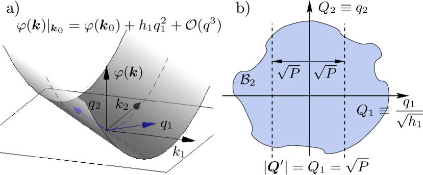
We can also treat the case where the Hesse matrix has only n () nonzero eigenvalues . With the transformations (, ) and , the contribution from a vicinity of becomes (see Fig. 1)
(13)
where , , and
.
Integral (13) has again the form of a Fourier transform and vanishes for , if . If is bounded in the vicinity of , the integral vanishes as . Those conditions on have to be interpreted as stricter conditions on when approaching zeros of , appropriate to still guarantee the dephasing. Zeros of with multiplicity () can be treated in a general fashion only for 1d by substituting . In higher dimensions they are a lot more complicated; see e.g. Varchenko1976 for 2d.
Figure 1: Sketch of coordinate transformation and integration path in (13) for a non-isolated zero of with , .
In the cases discussed so far, we have assumed that is continuously differentiable (). For the sake of brevity we will consider now only the scenario . This is for nondifferentiable. The cases and cover very typical examples (for example magnons, phonons or free particles). The contribution of a (small) sphere of radius around to the integral in (11) is with the substitution
(14)
This contribution vanishes for if and if is bounded, the contribution is of .
For a few general, physically relevant scenarios, we have established sufficient conditions under which (every matrix element of) the integral in (11) goes to zero as . As is finite and as we have a finite number of bands , those conditions guarantee hence that all nondiagonal contributions to vanish.
Due to Wick’s theorem, expectation values of arbitrary observables on are given by polynomials in . Nondiagonal contributions to will consequently also vanish if we restrict to finite subsystem sizes.
From the convergence follows then the proposition (6). Finally, (7) follows from and .
Preconditions.
During the proof, we collected the following prerequisites, sufficient to guarantee convergence to the steady state (6):
(a) is finite and .
(b) The parameterization of the quantum numbers is possible with a finite and a finite number of bands .
(c.1) , finite on , and . If this is not given for the vicinity of a point , we require for such a point
(c.2) if , then the Hesse matrix exists and is nonzero, and , or
(c.3) if, at , then . Of course, (c.3) can be generalized to the case with some nonzero matrix .
With those conditions, all nondiagonal contributions to the subsystem Green’s function matrix vanish for and dephasing to the steady state ensemble is effective, (6). If , , and are, in the corresponding situations, bounded instead of only integrable, nondiagonal contributions to decay (more quickly) as . Below, we give illustrative examples. Among those are simple scenarios where some of the prerequisites are violated and dephasing does in fact not occur.
Examples and counter-examples for dephasing.–
At the end of the proof, a reason for requiring (a) was given. A simple counter-example consists in violating (a) with and measuring , i.e. measurements in infinite subsystems, can reveal the phases and nondiagonal contributions (“rephasing”).
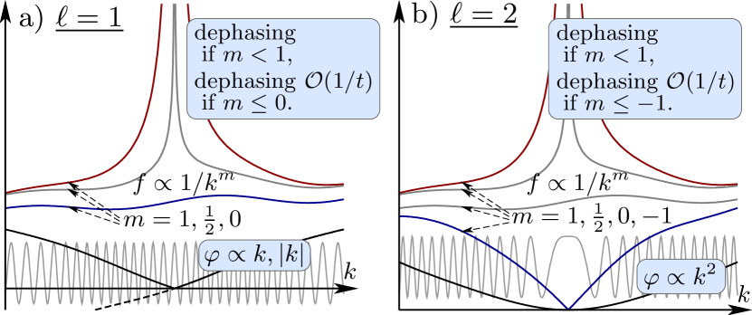
If has zeros or if has divergences, dephasing properties are dominated by the vicinities of such points. Thus, we illustrate (c) by considering the paradigmatic scenario , near (for some fixed and ). The integral in (11) is then
(15)
Hence this (nondiagonal) contribution to , for ,
does not vanish if , vanishes as if , and (at least) as if ; see Fig. 2.
In this scenario, both (c.2) and (c.3) apply with and are not only sufficient but also necessary.
Our first explicit example is (, )
(16)
the dimerized fermionic tight-binding model,
where modes and are coupled and the dispersion relation is , i.e. gapless if . The eigenmodes are labeled .
We evolve the groundstate for a certain dimerization with a different value . Skipping details of the calculation, we note that, using (11), the nondiagonal contributions from and to can be written as
(17)
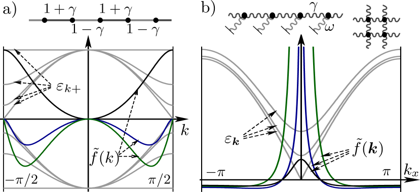
Fig. 3a displays and for and three different quenches with . The zeros of are and have each, in the notation of the paradigmatic situation (15), one of the characteristics . Hence, and dephasing of is guaranteed. The same is given for all other and has also been checked numerically. However, if we switch to , is const. and no dephasing can occur – we have uncoupled dimers.
Figure 2: Phase function , , and the nondiagonal
contribution to in the paradigmatic case (15), .Figure 3: a) Dimerized fermionic 1d tight-binding model (16). Dispersion relation for and the nondiagonal contribution to according to Eq. (17) for quenches (top to bottom).
b) The -dimensional harmonic lattice model. Dispersion relation for with , and the nondiagonal contribution to according to Eq. (19) for quenches (top to bottom).
As a second explicit example we choose the harmonic lattice model in dimensions (, ). Contrary to the first example, it will not dephase in all cases.
(18)
The dispersion relation is , i.e. gapless for .
With the bosonic operators , is brought to the form (2) and is hence amenable to the theorem. Using (11) we arrive at
(19)
where we switch at the oscillator frequency and
is the dispersion relation before that quench. The dephasing properties are dominated by the vicinity of .
If one switches between two noncritical values , its characteristic in terms of (15) is , i.e. and hence dephasing of for and for .
For , , one has and consequently no dephasing for , and dephasing of [] for [].
For , , one has and hence no dephasing for , and dephasing of for ; Fig. 3b. This was confirmed numerically for .
As a last example, consider free hard-core bosons in a 1d box. The system is prepared in the groundstate for a box of size which is switched to at , Rigol2007-98 . The Jordan-Wigner transformation yields a model of free fermions. The transformation between one-particle eigenstates before and after the quench ( and ) is
(20)
The weight of is concentrated in the interval . With the Fermi momentum , the initial Green’s function is diagonal in the basis and , which appears in (10), is hence also concentrated in . Thus and are and dephasing is ineffective. In Rigol2007-98 , the bosonic momentum distribution was found to relax to the one of the corresponding steady state ensemble . However, as the dephasing is ineffective, relaxation (6) of subsystem density matrices does not occur. This is also visible in the observables: As derived in Gangardt2007 , correlators do not relax to the value predicted by ; see also non-decaying oscillations of in Ref. 41 of Rigol2007-98 and Fig. 10 of Rigol2006-74 . That a particular observable, here , may relax anyway is a different issue. In Gangardt2007 it was shown for a slightly modified setup how relaxation of occurs.
Discussion.–
The dephasing theorem (6) confirms the conjectured (1), clarifies its interpretation, and devises conditions for its applicability. Dephasing properties are determined in particular by points where the gradient of the phase function, (12), vanishes or the amplitude , (10), diverges.
Also note that the notion of integrals of motion standing in involution as used for classical systems does not carry over to quantum mechanics, Weigert1992-56 . Hence it was per se not clear what operators were to be chosen in the maximum entropy ensemble (1). The theorem settles this question.
Further, as , (7), becomes finite for finite regions, the subsystem (entanglement) entropies will finally be dominated by the extensive contribution (cmp. to Calabrese2005 for 1d).
Hence, the required computational resources to simulate such systems on classical computers scale exponentially in the system size, preventing access to arbitrarily long times. On the other hand, this shows that quenches are a simple tool for the controlled generation of strong (extensive) entanglement.
Bethe Ansatz integrable systems.–
In Bethe Ansatz solvable models
Zachary1996 ,
the transfer matrix is conserved for any value of the spectral parameter ;
and
.
Initial states can be expanded in a -eigenbasis and, via time evolution, nondiagonal contributions will attain quickly oscillating phases
.
It will be shown elsewhere that, as in the free case, the nondiagonal contributions to the density matrix of a finite subsystem will under appropriate preconditions decay. Then, the steady state in the thermodynamic limit will, in generalization of (6), be given by
where denotes the density of quasiparticles.
Nonintegrable systems.–
Whether or how thermalization occurs in nonintegrable systems is in general unclear.
Intuitively, information about the initial state gets smeared out by scattering events which are, contrary to the integrable case Mussardo1992-218 , able to change the quantum numbers of the involved particles and not factorizable.
Our results are expected to carry over to nonintegrable cases, if system and initial state allow for a description by an integrable theory of quasiparticles (e.g. Fermi gases and Luttinger liquids) and quasiparticle lifetimes exceed time scales necessary to observe dephasing. In such cases, first relaxation to the steady state of the integrable theory will occur, followed by decay to the thermal ensemble.
Numerical results in Kollath2007-98 may be interpreted in this vein.
T. B. thanks the DFG and the Studienstiftung des deutschen Volkes for support.
References
(1)
E. T. Jaynes, Phys. Rev. 106, 620 (1957).
(2)
T. Kinoshita, T. Wenger, and D. S. Weiss, Nature 440, 900 (2006).
(3)
M. Rigol et al., Phys. Rev. Lett. 98,
050405 (2007).
(4)
M. Rigol, A. Muramatsu, and M. Olshanii, Phys. Rev. A 74, 053616
(2006).
(5)
M. A. Cazalilla, Phys. Rev. Lett. 97, 156403 (2006).
(6)
M. Eckstein and M. Kollar, arXiv:0707.2789.
(7)
D. M. Gangardt and M. Pustilnik, arXiv:0709.2374.
(8)
M. Cramer et al., Phys. Rev. Lett. 100, 030602 (2008).
(9)
A. Varchenko, Funct. Anal. Appl. 10, 175 (1976).
(10)
S. Weigert, Physica D 56, 107 (1992).
(11)
P. Calabrese and J. Cardy, J. Stat. Mech. P04010 (2005).
(12)
N.-C. H. Zachary, Quantum Many-Body Systems in One Dimension (World
Scientific, Singapore, 1996).
(13)
G. Mussardo, Phys. Rep. 218, 215 (1992).
(14)
C. Kollath, A. M. Läuchli, and E. Altman, Phys. Rev. Lett. 98, 180601
(2007).