KUNS-2112
Higher Order Couplings
from
Heterotic Orbifold Theory
We calculate couplings of arbitrary order from correlation functions among twisted strings, using conformal field theory. Twisted strings arise in heterotic string compactified on orbifolds yielding matter fields in the low energy limit. We calculate completely the classical and the quantum amplitude including normalization, up to a contribution from Kähler potential. The classical action has saddle points which are interpreted as worldsheet instantons described by metastable untwisted strings, formed by twisted strings distributed at certain fixed points. This understanding generalizes the area rule, in the case that the locations of twisted strings do not form a polygon, and provides a general rule for calculating these kinds of instanton corrections. An interpretation of couplings involving linearly combined states is given, which commonly appear in non-prime order orbifolds. The quantum part of the amplitude is given by ratios of gamma functions with order one arguments.
1 Introduction
Superstring theory is a promising candidate for unified theory including gravity. Heterotic orbifold construction is one of interesting constructions for four dimensional string models [1, 2]. (See also for resent works Ref. [3, 4] and for review [5].) One can solve equation of motion of string on the orbifold background, and geometrical picture is clear in heterotic orbifold models. Thus, several aspects can be computed and can be understood from the geometrical viewpoint.
Heterotic orbifold models have modes localized at fixed points, that is, twisted strings. 3-point couplings as well as 4-point couplings of these localized modes have been computed analytically [6, 7, 8, 9, 10], and the size of Yukawa coupling is obtained as , where denotes naively the area of triangle corresponding to three fixed points of twisted strings. This will be clarified more and generalized in this paper. This aspect is quite interesting from the phenomenological viewpoint. One can obtain suppressed Yukawa couplings when twisted strings are localized far away from each other. That is, one could explain the hierarchy of quark and lepton masses as well as their mixing angles when they are localized at different places.
We have to study selection rules for allowed couplings in order to examine whether realistic fermion masses and mixing angels can be realized from string theory. The space group selection rule [7, 11] constrain allowed Yukawa couplings rather strongly. For example, on prime order orbifolds off-diagonal Yukawa couplings are not allowed, and we can not obtain realistic mixing angles by using only 3-point couplings with the minimum number of Higgs fields.111In non-factorizable orbifold models, off-diagonal Yukawa couplings are allowed, but it is still difficult to derive realistic Yukawa matrices [12]. On non-prime order orbifolds, off-diagonal Yukawa couplings are allowed [11] and possibilities for leading to realistic quark and lepton masses and mixing angles have been studied [13]. However, to realize fermion masses and mixing angles in string theory is still a challenging issue.
In this paper, we study generic higher order couplings than renormalizable couplings in heterotic orbifold models. Higher dimensional operators become effective Yukawa couplings after symmetry breaking. Suppose that we have a coupling of type in the superpotential of effective field theory, where and are chiral matter fields corresponding quarks and leptons, denotes electroweak Higgs superfields and correspond to several heavy modes. When all scalar components of the superfields develop their vacuum expectation values (VEVs), this higher dimensional operator becomes a Yukawa coupling among chiral fermions and and the electroweak Higgs fields . Thus, there is a possibility for deriving quark/lepton masses and mixing angles through this type of symmetry breaking, but by use of not only 3-point couplings. Indeed, such possibility has been examined in explicit models [2, 3, 4]. Therefore, it is important to study selection rules of allowed higher order couplings and compute magnitude of allowed couplings.222 It would also be useful to study non-Abelian flavor symmetries [14, 15] and accidental global symmetries [16] in string models. When correspond to localized modes on orbifold fixed points, the above effective Yukawa coupling may correspond to a 3-point coupling on a Calabi-Yau manifold, where orbifold singularities are smoothed by the VEVs of . Thus, calculations of higher order couplings on the orbifold are also important from the viewpoint of calculations of 3-point couplings on the Calabi-Yau manifold around the orbifold limit.
We compute magnitudes of -point couplings. Generic aspects of -point couplings heterotic orbifold models have been obtained in [8]. Here we apply it to concrete heterotic orbifold models. Similar calculation has been carried out for generic -point couplings in intersecting D-brane models [17].333See for 3-point couplings in intersecting D-brane models [18, 19, 20, 21].
The paper is organized as follows. In section 2, we give a brief review on heterotic orbifold models in order to fix our notation. Then, we study the selection rule due to discrete -symmetry and the space group. In section 3, we compute classical contributions of -point couplings. Their quantum parts are calculated in section 4. In section 5, we consider normalization of correlation functions. Section 6 is devoted to conclusion and discussion. In appendix, we give useful formulae for hypergeometric functions and their multivariable generalizations.
2 Setup
2.1 Twisted strings and their vertex operators
The heterotic string theory consists of 10D right-moving superstring and 26D left-moving bosonic string. For the common ten (bosonic) dimensions, we consider the background with our 4D space-time and 6D orbifold. The other 16D left-moving bosonic string correspond to a gauge part. A 6D orbifold is a division of a 6D torus by a twist , while is obtained as , where is a 6D lattice. The twist must be an automorphism of the lattice , and its eigenvalues are diag in the complex basis . We mainly concentrate ourselves to the case that is factorizable as . To preserve 4D supersymmetry (SUSY), they must satisfy the following condition,
| (1) |
where is not integer for each .
The twisted string is a closed string up to orbifold identification
| (2) |
where is the above lattice (in the complex basis) defining the orbifold. It makes sense to restrict the phase to be . Its zero mode satisfies the same condition, and it is called a fixed point on the orbifold. The fixed point can be represented by the corresponding space group element, . Note that the fixed point is equivalent to . They belong to the same conjugacy class. The sector with corresponds to the so-called untwisted sector.
The local operator called the twist operator takes into account the nontrivial boundary condition (2) by inducing a branch point at with the order on the world-sheet, but the theory remains local by moding out by orbifold projection. The ground state corresponding to the twisted string on the fixed point is generated from the untwisted ground state by the twist field . These twist fields have the operator product expansions (OPEs)
| (3) | ||||
| (4) |
which are understood as the most singular parts in the mode expansion for . For the other region , we have the corresponding relations by replacing with . Also we have similar expressions for . Their conformal weights for the holomorphic and anti-holomorphic parts are
| (5) |
thus inducing a shift of zero point energy.
Each -twisted sector has several ground states, that is, twist fields corresponding to several fixed points under twist. When we specify the fixed point , we denote . Also we use the notation , where denotes the space group element corresponding to the fixed point under twist.
On non-prime order orbifolds, fixed points under higher twist () are not always fixed under or twist fields are not always eigenstates of the twist . To make eigenstates, we have to take the following linear combinations [22, 11],
| (6) |
where with integer to be determined by gauge quantum numbers and internal momenta. This linear combination may include twist fields corresponding to fixed points, which belong to the same conjugacy class.
We consider the covariant quantization with the explicit conformal and superconformal ghosts. It is convenient to bosonize right-moving fermionic string and write bosonized degrees of freedom by . In the bosonized formulation, untwisted massless modes have momenta for , which are quantized on the weight lattice. The space-time boson and fermion correspond to vector and spinor, respectively. The compact space corresponds to . The twisted sector has shifted momenta, , which are often called -momenta.
A bosonic massless state has the corresponding vertex operator,
| (7) |
naturally in the -picture, where is the bosonized ghost, corresponds to the gauge part and corresponds to 4D part. Here, and denote oscillators for the left-mover, and and are oscillator numbers, which these massless modes include. Similarly, we can write massless modes corresponding to space-time fermions as
| (8) |
in the -picture. We understand that the fields contains the four dimensional spin field. The -momenta for space-time fermion and boson, and in the same supersymmetric multiplet are related each other
| (9) |
that is, corresponds to the -momentum of unbroken 4D space-time SUSY charge. To each vertex operator, we have to include overall normalization
| (10) |
from the state-operator mapping or the unitarity relation [23]. The closed string coupling is expressed in terms of ten dimensional gauge and gravitational couplings
| (11) |
Thus, including one more field suppresses the corresponding coupling by one inverse mass dimension as we expect. We have omitted the two-cocycles, which determine the overall sign [24].
We calculate a correlation function among twisted matter fields including two space-time fermions on the orbifold, along the lines [7, 8, 9, 17]. It yields a higher order coupling in the zero momentum limit . Since the background has the superconformal ghost charge 2, the correlation function is of the form,
| (12) |
such that the total ghost charge vanishes. Here is worldsheet cosmological constant and we also have three bosonic ghost fields and . We take radial ordering implicitly, which reflects the ordering property from noncommutative space group.
In order to make the total superconformal ghost charge vanishing, we need vertex operators in the -picture. We can obtain by operating the following picture changing operator on [25],
| (13) |
where , and for the components corresponding to the 6D compact space. Thus we have
| (14) |
up to the same normalization (10). Here, is the th component of . Containing no derivatives, the higher order coupling is defined in the zero momentum limit . Thus the first term is not relevant. The only change is that some components of twist fields are replaced by excited twist fields , and the normalization factors , in accord with the number of oscillators in (10). In the next subsection, we see this change does not modify the calculation in the case that all the twist fields are simply , not excited twist fields.
2.2 Selection rules
Here we briefly summarize the selection rules [7, 11, 3, 26, 27]. The vertex operator consists of several parts, the 4D part , the gauge part , the 6D twist field , the 6D left-moving oscillators and the bosonized fermion , as explained in the previous subsection. Each part has its own selection rule for allowed couplings. The selection rules of the 4D part and the gauge part are simple, that is, the 4D total momentum and the total momentum of the gauge part should be conserved. The latter rule is nothing but the requirement of gauge invariance. The other parts lead to non-trivial selection rules. In this subsection, we study the selection rule from the -momenta and oscillators, as well as the selection rule from the 6D twist fields .
The total -momentum should be conserved like the 4D momentum and the gauge momentum . For example, for 3-point couplings , they should satisfy the following condition,
| (15) |
Here we take a summation over the -momentum for the scalar components, using the fact that the -momentum of fermionic component differs by .
Another important symmetry is the twist symmetry of oscillators. We consider the following twist of oscillators,
| (16) | |||
| (17) |
without summation over each . Allowed 3-point couplings should be invariant under the above twist.
However, for generic -point couplings we have to carry out picture changing, and the picture changing operator includes non-vanishing -momenta and right-moving oscillators and . Thus, the definition of -momentum depends on the choice of the picture. However, the R-charges, which are defined as [3]444See also [28] and references therein.
| (18) |
are invariant under picture-changing. Here we do not distinguish oscillator numbers for the left-movers and right-movers, because they have the same phase under twist. Indeed, physical states with picture have vanishing oscillator number for the right-movers, while the oscillator number for the left-movers can be non-vanishing. Thus, hereafter and denote the oscillator number for the left-movers, because we study the physical states with picture from now. For simplicity, we use the notation . Now, the selection rule due to R-symmetry is written as
| (19) |
where is the minimum integer satisfying , where with any integer . For example, for -II orbifold, we have , and .
Whereas the twist operator itself does not transform under the twist of oscillators, the excited twist operator transforms like the oscillator in (16), since it is nothing but the product of an oscillator and a twist operator, from the transformational point of view. The modified -momentum has a compensating property and the resulting amplitude is invariant under the twist of oscillators, as it must be because the picture changing operator is invariant. However the OPE is of a similar form of a twisted operator
| (20) |
which is readily extracted from the OPE . It has a branch structure like , but the part is carried by from its definition to leave (20). Thus the amplitude including excited twisted operators is the same as one including only twisted operators, up to the overall normalization.
We have the space group selection rule. Here, we study the selection rule for twist fields, . First of all, the product of phases should satisfy .555That is automatic for physical states when the other selection rules are satisfied [26, 27]. Next, we study the space group selection rule. Now, let us consider -point couplings of twisted states corresponding to (). Their couplings are allowed if the product of space group is the identity, i.e.,
| (21) |
Since space group elements do not commute, nor do vertex operators, the ordering of vertex operators in the coupling is important. We have to take into account the fact that is equivalent to . Thus, the condition for allowed couplings is that the product of space group elements must be the identity up to such equivalence. The space group selection rule includes the point group selection rule, which requires , i.e. (mod ) for the orbifold. The rules for the linearly combined states are discussed in detail in Ref [27].
3 The classical contribution
Here we consider the 6D orbifolds, which can be factorized as three 2D orbifolds, and we concentrate ourselves to calculation of correlation functions on the 2D orbifolds. The following analysis can be extended to other cases, where 6D orbifold is not factorizable or 6D orbifold includes 4D non-factorizable orbifold.
The nontrivial part is the correlation function among twist operators
| (22) |
This can be calculated independently of the remaining components of vertex operators, because they commute. Some of them should be excited twisted states for the total ghost charge being . Indeed we noted above that the amplitude is the same with a number of factors .
From the point group selection rule we have
| (23) |
where must be an integer. For the moment we assume
| (24) |
and we will relax this condition later. This choice is the most convenient one because of two reasons. First, by doubling trick we can relate the corresponding amplitude with that of open strings [17], where this is the closedness condition for sided polygon. This gives rise to the generalized Schwarz–Christoffel transformation and the area rule that we will show below. Another reason is that we can obtain the closed form of integration, in terms of a multivariable hypergeometric function [29].
If we use path integral formulation, the correlation function (22) is divided as
| (25) |
according the classical value and the quantum fluctuation around it, i.e. .
The corresponding tree-level Feynman diagram is a sphere with a number of vertex operators inserted. Every object in string theory, including the vertex operators and the correlation function (22) can be separated into holomorphic and antiholomorphic part. Considering one of them, holomorphicity restricts many things in a very simple form. Using the compactification we can cover all the coordinate on the sphere by holomorphic coordinate except infinity. To take care of infinity we introduce another patch where becomes . Considering a holomorphic solution from
| (26) |
if we need the LHS well-behaved at , in the RHS should drop faster than as goes to infinity.
3.1 -point coupling
We begin calculating the classical contribution first. We see that the classical solution is the completely factorized part for each inserted operator. Therefore, from the OPEs (3) and (4), the classical solutions are obtained by the holomorphicity and the desired singular structures as
| (27) |
Here we define the basis of functions
| (28) |
For the symmetric orbifold they are complete since and . From (26), the whole part (27) should behave as as . Using (24), we can see does. For , we admitted an additional degree of freedom, i.e. changing the power of singularity by integer, since it does not modify the branch cut structure. Hence, we have many free parameters .
To determine the coefficients , we should consider the global monodromy condition. The relation (2) does not take into account the global phase if we transport branch cuts from more than one fields. Taking a contour encircling more than one points gives the relation between overall coefficients in (27) and net translation in the target space
| (29) |
This expression makes sense only if there is no additional phase. The quantum part does not carry any amplitude . Hence, Eq. (29) shows a purely classical contribution. Upon integration relating these branch cuts, the Pochhammer loop [30] is a clever way to encompass the two branch points nontrivially without phase. For each branch cut the contour goes in and out exactly once through the cuts, depicted in Fig. 1. Its effect is to encircle the fixed points: clockwise, counterclockwise, counterclockwise and then clockwise. In terms of space group elements and with , we obtain
| (30) |
where . The encircling is not necessarily once, i.e, in general, in which we cannot draw branch cuts. The net effect is pure translation. It turns out that every contour is generated by the basis of Pochhammer loops encircling -th and -th points.

Taking Pochhammer loops around the vertices and , from (30) we obtain
| (31) |
We have vectors and angles (with the constraint (24)), which completely specify -sided polygon.
Later we can express the solution in terms of the following integrals
| (32) |
and
| (33) |
with
| (34) |
Note that and form matrices. In Appendix, they are expressed in terms of multi-valued hypergeometric functions [17, 29]. With , we can set to be respectively and the others to the cross-ratios of .
Plugging (27), the solution is expressed as
| (35) |
where we defined , and by inverting them we obtain
| (36) |
where the inverse is taken with respect to the matrix basis with indices . Plugging into the classical action, we obtain the final solution
| (37) |
where
| (38) |
We can expand this action by products of holomorphic and antiholomorphic functions, with careful choices of contours. It is nothing but the relation between open and closed string amplitudes before integration over s [31],
| (39) |
where
| (40) |
Plugging in (37), we obtain the classical action . It it a function of complex variables which will be integrated out in the final amplitude. Later, we will integrate this with variables over the entire complex plane. Among these, using the saddle point approximation by adjusting s or equivalently ratios , we find a minimum
| (41) |
Note that in general the integrals are complex and we coordinated the fixed points as complex vectors on a given 2D torus and orbifold.
Inserting these into (36), we have for all , except . The solution is nothing but the generalized Schwarz–Christoffel transformation [29], whose original version maps the upper half plane into inside an -polygon
| (42) |
Namely, the points are mapped to vertex and the turning around angle is given by . In this case, we obtain the instanton contribution is exponential of the polygon area
| (43) |
This is valid under the assumption (24), i.e. forming a polygon, but in general case we have more fundamental interpretation shortly.
Of course, there are other minima with the same value, where and all vanish except one, say . This corresponds to and the Schwarz–Christoffel transformation corresponds to .
In forming the area from the Schwarz–Christoffel transformation, the ordering is important. If we just exchange two fields, we cannot satisfy the space group selection rule in general, and the polygon becomes self-crossing, where the area rule is not applicable. In the correlation function we take the radial ordering. In the superpotential of effective field theory, we do not see the ordering, since the integration over all completely symmetrize the amplitude.
3.2 Four-point correlation function
The four-point correlation function provides a good example of calculation of the classical part. In this case, the functions are well-known hypergeometric functions, which are solutions of second order linear differential equation. It is known [32] that if any three of the solutions have the common domain of existence, there be a linear relation among them. In our case, we can express all of in terms of, say, and . They are shown in (A) and (A) of Appendix.
Plugging these to (39) the holomorphic part is obtained as
| (44) |
where
| (45) | ||||
The coefficient reduces to
| (46) |
only for the polygon case, using (24). The prefactor in is the relative phase of (complex numbers) and , where with . From (36) we have the coefficients
| (47) |
We can obtain the antiholomorphic action and integral from and respectively, by substituting and . With these we obtain the classical action (37). The action does not have manifest duality symmetry, since we have fixed four points by .
We define the following modulus
| (48) |
which is in the case the modular parameter of two-torus, made by connecting two Riemann sheets with two branch cuts [6, 7]. As expected from (41), the minimum of is obtained at
| (49) |
Thus we have and the minimum of classical action is obtained as
| (50) |
For the case of polygon, the classical action reduces to
| (51) |
This is the area of the quadrilateral formed by vertices at the fixed points and .
In the case with and/or , this expression is not well-defined. Without loss of generality, the case with and leads to , by use of (24), and such a case has been calculated in [7]. Here we have to come back to (44), and the result agrees.666 To compare between our results and [7], we have to replace our modulus by . The case with or leads to , and such a case has been calculated in [9].
From four-point amplitude, we can obtain three point amplitude by taking to, say, . In this case the fixed points and become coalescent and the classical action reduces to
| (52) |
Note that this action depends on the choice of contour “picture”. Here, we chose one encircling two fixed points and . We do not need worry about whether is actually compatible to factorization [7]. The Pochhammer loops in which and belong are independent.
In the special case with , we have and yielding
| (53) |
which is again interpreted as twice the area of the rectangle, in unit of if is orthogonal to . This is the case of order 2 subsector (-th twisted sector) in even order orbifold. Note that this action is not the minimum action, since in this case the classical action is not the function of . In this case the area rule interpretation is somehow ambiguous. We will study more detail in the following subsection.
We have considered -point couplings only for as examples. However, we will study that higher order -couplings reduce to a combination of lower order -couplings with by the discussion of field coalesce in subsection 3.4. In addition, since the number of fixed points on orbifolds is limited, we can expect that most of higher order -couplings can be written as combinations of -point couplings only with . We will study this expectation in separated papers [27, 33], by examining concrete orbifold models.
3.3 Non-polygon case: the meaning of area
We assumed the polygon condition (24) is satisfied. However, in general, the following relation
| (54) |
is possible. In the inequality case, the holomorphic part of the classical solution decays faster than , whereas the antiholomorphic part decays not faster than . The only sensible way of treating is to make antiholomorphic part vanishing.
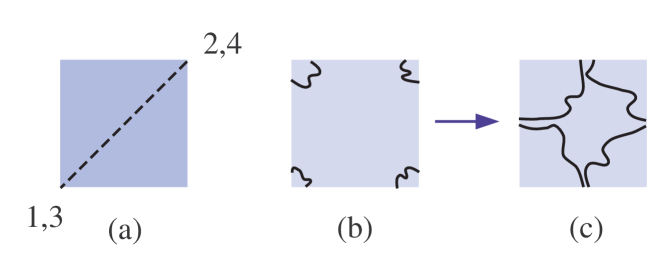
For example, in the orbifold, the coupling of four first twisted sector fields,
shown in Fig. 2(a), satisfies the space group selection rule. Note that does not satisfy the space group selection rule, and the ordering is important. All of twist fields are of order four, which cannot satisfy the relation (24). The classical solution is obtained as
| (55) |
From global monodromy condition, we have
and the classical action is given with , yielding
Thus we have the classical contribution
which is interpreted as the area of the square whose diagonal is .
Similarly, for the coupling
we obtain the classical action,
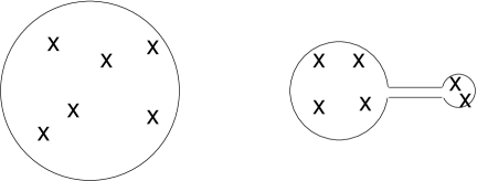
In these cases, we have a different area rule: The “area” is not that surrounded by fixed points, but one as follows. The classical solution describes a local minimum of the action, which is the instanton of worldsheet nature, suppressed by . The selection rule tells us that these twisted strings can potentially make an untwisted string, which is not possible due to energetics for massless strings, since they are completely localized at certain fixed points, as in Fig. 2(b). However they can oscillate to grow to be large size, and above a certain threshold, they can form an untwisted string as in Fig 2(c). Noting that the instanton describes tunneling between vacua which is energetically forbidden, we can understand that forming untwisted string corresponds to such tunneling.
Still we can have the hint from the modified area. It is the sweeping area for localized twisted strings to grow to become a untwisted string. For the polygon case, i.e. that satisfying the condition (24), this interpretation is still valid, since still the area swept by twisted strings at each vertex makes the polygon area.
On the other hand, in the case not satisfying the condition (24), we lost the interpretation of the mapping being a generalized Schwarz–Christoffel transformation, since in the target space the fixed points fail to make a polygon.
The subleading correction is generated by identical fixed points on the orbifold, but more separated in the covering space, i.e. . Since they are identical points, they satisfy the selection rule. With this interpretation, we can understand the classical solution which makes more than one untwisted strings possible. For example, for , the coupling , where each fixed point belongs to the same conjugacy class as the previous one, satisfies the space group selection rule, but corresponds to a large and a large instanton action.
3.4 Fields coalescent at the same fixed point
In most cases, some of the fields sit at the same fixed point . The corresponding correlation function might be obtained by taking the limit in the correlation function,
| (56) |
Note that this limit is not always well-defined. It is because twist fields do not commute. By conformal symmetry, the OPE has the generic form,
| (57) |
Equating the conformal weights of the both sides, we have
| (58) |
Because of the nontrivial branch cut, this relation is asymmetric under the exchange of two twist fields. This property is also reflected in the space group elements, which do not commute, either. We can define an invariant block of twist fields, which correspond to the identity of the space group . Thus, these invariant blocks commute and satisfy
| (59) |
In the case where two points and are in the successive order, and we can merge two twists without ruining the radial ordering. They are neighboring points as polygon vertices. Then, from (57) the two twists reduce to a single twist with the summed order. Also this implies the classical solution becomes
| (60) |
where, again, the even integral power is not relevant to branch structure, so that we can make lie in for instance. This means, not all of vertices form the -polygon, but effectively one with the lesser vertices. (Recall that the positions of vertices are given as singularities in the classical solution.) In fact this is the familiar case when we obtain a three point function from the four point function by setting two of the points coalesce. In the latter limit, the polygon is triangle. We can see this in terms of space group elements. Neglecting gauge group, which is not involved in the classical amplitude, we cannot distinguish the product
| (61) |
when two identical twisted fields sit at the same point, and are put on the neighboring points in the correlation function.
There is the case where is integer. In this case there is no singularity in the classical solution and such vertex does not contribute to the area rule. In the extreme case where order- twisted fields sit at the same points, the coefficients of higher order couplings are not suppressed. Thus all we need to consider is the other nontrivial couplings. Fortunately, not all of them survive: From -symmetry invariance, the correlation function is further constrained.
However, from the radial ordering, there is a case in which the exchange of two branch cut fails to give well-defined radial ordering. This is not possible for two fields which are not the neighboring fields in the correlation function, since the space group and the mapping of classical solution is not commutative.
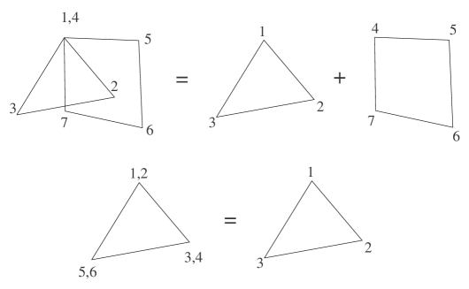
For example, in couplings among twist fields corresponding to two ’s, two ’s and two ’s on the orbifold, there are two following combinations possible, satisfying the space group selection rule
| (62) | ||||
| (63) |
In the first case, the solution behaves like
| (64) |
The two points, and for , correspond to the same fixed points on the target space, i.e. , and . Thus, we take the limit for . In such a limit, the solution behaves like
| (65) |
Thus, in the space group point of view, it is indistinguishable from the coupling among the second twisted couplings
| (66) |
which gives only the area of triangle. On the other hand, the latter coupling (63) gives twice the area of the triangle. The classical solution maps from the different points to the same points. For example the holomorphic part behaves
| (67) |
and the two points, and for , correspond to the same fixed points on the target space, i.e. , and . Otherwise the ordering is ruined. It is also understood that two different and independent sets of twisted fields can sweep the triangle, which means the instanton corrections from the complete polygons are additive in the action. This case is depicted in Fig. 4.
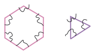
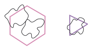
We summarize how to calculate the classical part of -point couplings among twist fields (). First, we classify all of possible ordering of these twist fields, which satisfy the space group selection rule. For each ordering of twist fields allowed by the space group selection rule, we consider the following procedure. We combine two or more twist fields sitting at the same fixed point to a single twist field like (57) and Fig. 3 if possible, that is, they satisfy (59). When their total twist is just twist with integer , correlation function reduces to much simpler form. The resultant correlation function can be written as product of invariant blocks, which satisfy the space group selection rule like Fig. 3. Each block includes smaller number of twist fields.777 In most of cases, may be equal to . We will study this point in concrete models [33]. Then, for each block, we calculate classical contributions, , i.e. instanton actions corresponding to the minimum action and larger ones, and take their summation, i.e. . Next, we take a production of classical contributions corresponding to each block, i.e.
| (68) |
Finally, we sum over all of possible ordering to obtain the total coupling, i.e,
| (69) |
Because of the ordering, the correlation function does not possess the worldsheet duality like in the Virasoro–Shapiro amplitude [34]. In the vanishing momentum limit we do not distinguish the channel, thus the effective coupling like Yukawa coupling does not distinguish the order. However even in this case, the above two cases are distinguishable, since this contribution is the worldsheet effect, suppressed by .
3.5 Linearly combined states
In higher order twisted sector of a non-prime order orbifold, there are states formed by linear combinations, as in (6) , due to the orbifold projection. The linear combination of states can be more precisely defined by that of vertex operators. It follows that the corresponding classical solution consists of linear combination of individual solutions before combination, and also the relative weights are inherited. For example the classical solution involving (6) contains the factor
| (70) |
where is mapped to the fixed points .
For such couplings, we observe two points
-
1.
The selection rule for a linearly combined state is derived from that for each term.
-
2.
A part of the classical solution, which does not satisfy the selection rule vanish.
The proof for the first is given in Ref. [27], and we easily see the latter is the case. We can show that such term not satisfying the classical solution always contain the same element more than once. Setting these to the other(s) corresponding to shrinking the area to zero, if we do not want to change the angles corresponding other vertices.
For instance, in the second twisted sector of orbifold, we have a coupling including linearly combined states
| (71) |
The total coupling is given by summation over each of the four correlation functions. However, the nonvanishing contributions come from the only ones satisfying the selection rule. One that does not satisfy the rule, e.g. , does not contribute.
To sum up, for the linearly combined state, we can treat a linearly combined state as a complete physical field, the classical amplitude has only contribution from the parts satisfying the space group selection rule.
4 The quantum amplitude
Now we determine the quantum part of the amplitude (25),
| (72) |
We use the stress tensor method [7, 9, 17], in which (72) can be indirectly calculated, relying on only the holomorphicity. All the information can be read from the Green’s function
| (73) |
Its form we know from the holomorphic part of the OPE (3),
| (74) |
where . The condition avoids overcounting, although otherwise the formula would be more symmetric. The prefactor , from (28), gives the desired pole structure. The normalization is determined by requiring the limit of to be 1, and the condition
| (75) |
leads the desired conformal weight , as the coefficient of each double pole in . To have no residue in , we require the condition for ,
| (76) |
where we use the fake number for the case . Summing over , this condition implies (75). We have less condition for many , reflecting the freedom of our choice of . Of course, the physics does not depend on the choice . As , we have the OPE
| (77) |
We extract the residue for fixed , and take limit.
In the limit , the Green’s function becomes energy-momentum (stress) tensor
| (78) |
where the last term arises from the normal ordering. Sandwiching the OPE in the correlation function
| (79) |
with the fixed and its conformal weight given in Eq. (5), we can completely calculate the holomorphic part up to normalization
| (80) |
We obtain
| (81) |
At this stage, using symmetry, we set . Then dependent terms vanish since , but there are corrections to this from , which are also dependent on . We now have unknown for constraint, and remaining freedom corresponds to redefinition of .
Similarly we define the antiholomorphic Green’s function
| (82) |
To obtain and , we apply the global monodromy condition for the quantum part
| (83) |
It is convenient to call the first term in the RHS (74) as . If all the are different, the matrix has the inverse. Thus we can multiply it to eliminate and , so that we obtain
| (84) |
Since we set , the only relevant terms are ones containing the factor . We divide them by and take the limit . Then, in the sense of (79), we read off the residue of in the integrand
| (85) |
where we have replaced with by the relation (76). Therefore we have no dependence on the specific choice of , or , as it should be.
Integration around the contour gives
| (86) |
The first term in the RHS is contained in the derivative of . By the chain rule, we obtain
| (87) |
For the second term in the RHS of (86), in the same way, we find the singular structure as ,
| (88) |
Thus we obtain
| (89) |
up to antiholomorphic action. In fact, there are additional factors, since we have used only the part of the terms in (87). The remaining terms completely vanish if we calculate the antiholomorphic part in the same way. The similar analysis is carried out for , by dividing by . Combining it with the holomorphic part , we arrive
| (90) |
up to the normalization, to be determined in the following section. The various branch cuts reflect the noncommutativity of the vertex operators under permutation, due to orbifold phase. As well as the classical part, the quantum part has no world-sheet duality, either. Nonetheless the complete amplitude will be single-valued, completed with other parts of vertex operators.
5 Factorization and normalization
To normalize the amplitude, we choose the reference of normalization
| (91) |
Equivalently, two twist fields of the opposite twists coalescent at the same point become the identity operator. In general we cannot make use of the normalization (91), since for each twist field we need one with the opposite twist. Thus we use a doubling trick.
First we calculate point function with twists
| (92) |
By setting we obtain the product of a -point function and a -point function. From the unitarity, the intermediate state gives an on-shell pole, with the lowest state being massless gauge bosons,
| (93) |
This factorization is schematically drawn in Fig. 5.
Concentrating only twist fields, the intermediate gauge boson does not contain a twist field. The former contains only twist operators and the latter has the form as in (91). Therefore we have
| (94) |
We have already known the general solution. For this we have the same action, including the classical and the quantum parts, except the factor . In this, each term contains the common factor
| (95) |
Thus there is a discrepancy between the two by the factor
| (96) |
where the subscript in the determinant indicates that these are for and point correlation functions, respectively. This is so, since the normalization of point function have no special dependence of a specific . In effect, we replace in (90) with , which is defined in (34). This is a desirable result, since any choice of factorization should give the same result, not depending on the special set of contour choice, which is reflected in .
We cannot go from the four-point function into the product of two two-point functions, since the point cannot be arbitrary close to all of , already fixed by , at the same time. For this, we do the Poisson resummation [7]. Since it involves a lattice transformation into its dual lattice, as a result we have the overall factor of the lattice volume.
Finally we set to infinity to obtain the OPE
| (97) |
where the selection rules should be satisfied. The RHS is nothing but the product of two identical th order couplings. Comparing the coefficients, we obtain the coupling of order
| (98) |
where
| (99) |
For the rest of vertex operator components, we have
| (100) | ||||
Multiplying these, and using the massless condition, the branch cuts disappear in the overall amplitude. Including universal geometric factor of sphere , we have the overall factor
| (101) |
up to contributions from picture changing and/or oscillator excitations (10). For the four point coupling, we have volume factor suppression from the compactification.
As the simple example, we can extract the information for three point correlation function. By symmetry, we can fix three arbitrary given points completely, thus the correlation function contains no information. To obtain it, we need four point correlation function with twists
| (102) |
where we consider only one two-torus. From (32), we have
| (103) |
Let us assume . In the limit , using the relations (110) and (111) in Appendix, the most dominant part has the coefficient
| (104) |
where we used the relation . Thus, taking the entire compact dimension, the Yukawa coupling is obtained as
| (105) |
with the classical action given in (52). For the case , we can obtain the corresponding amplitude by replacing by . It is notable that, in the quantum amplitude, there is no contribution from the geometry, since it is canceled by the same dependence in the four dimensional gauge coupling arising from the dimensional reduction.
We can obtain similar expressions for the higher order couplings, expressed in terms of multivalued hypergeometric functions. One can be convinced that the asymptotic form of generalized hypergeometric function in the above limit is the ratios of gamma functions [35] with arguments of . Thus we expect that the quantum parts of the higher order couplings are roughly of order one. Thus we see that the size of higher order coupling is dominated by the classical part.
6 Conclusions
We have calculated couplings of arbitrary order, among untwisted and twisted fields of heterotic string on orbifolds, using conformal field theory. In the low energy limit, they correspond to the matter superpotential. They are given by the zero external momentum limit of radially ordered correlation functions. The specification of orbifold and the shift vector determines the possible couplings. This provides us with lessons for constructing low-energy effective field theory, in particular for vacuum configurations of compactified string theory and realistic quark and lepton masses.
The higher order couplings are complicated due to two things. The first is the technical difficulties dealing with arbitrary number of twist fields and even some excited twist fields from the picture changing. In the calculation of higher order coupling, the latter has just an effect of changing the normalization, not changing the transformation property and the branch cut structure. The other difficulty arises from linearly combined states, which appear in higher twisted sectors of non-prime order orbifolds. They make the interpretation of the classical and the quantum somewhat tricky.
The selection rules (mainly studied in Ref. [27]) from the location of fields and the -symmetry can be possible origins of discrete quantum numbers in effective field theory. They also provides the understanding on discrete flavor symmetries. Because of the restrictive form of selection rules, in particular in the heterotic string models, only limited number of couplings are possible, since there are limited number of orbifolds and fixed points. This will be classified elsewhere [33].
The classical part is an instanton amplitude of world-sheet nature. Its size is exponentially suppressed by the effective area swept by the twisted strings to form untwisted strings. The latter is energetically not allowed, metastable intermediate state. This generalizes the naive area rule even if the twisted strings do not form a polygon. Decomposing the locations of twisted fields, we can obtain handy rule for calculating the size. For couplings involving linearly combined states, the only contribution comes from the terms satisfying the space group selection rule. The others vanish individually.
We have also calculated the quantum amplitude with the complete normalization, up to the Kähler normalization. In this there is no contribution from the geometric distribution of the fields, since the contributions from the normalization and that from the dimensional reduction cancel.
Besides the suppressions from the closed string couplings and oscillator normalizations, the coefficient is given by ratios of products of gamma function, whose argument is of , thus we expect a factor of from the quantum amplitude. The dominant amplitude is classical one, which is exponentially suppressed. Thus it is easy to generate hierarchy of Yukawa couplings. However, from the top-down approach, it is not easy to locate the desired fields at the desired positions.
Acknowledgements
We are grateful to Steve Abel, Massimo Bianchi, Jihn E. Kim, Hans-Peter Nilles, Saul Ramos-Sanchez, Michael Ratz, Robert Richter and Patrick K. S. Vaudrevange for discussion. K. S. C. thanks to Yukawa Institute for hospitality, where part of the work is done. K. S. C. is supported in part by the European Union 6th framework program MRTN-CT-2004-503069 “Quest for unification”, MRTN-CT-2004-005104 “ForcesUniverse”, MRTN-CT-2006-035863 “UniverseNet” and SFB-Transregio 33 “The Dark Univerese” by Deutsche Forschungsgemeinschaft (DFG). T. K. is supported in part by the Grand-in-Aid for Scientific Research #1754025 and the Grant-in-Aid for the 21st Century COE “The Center for Diversity and Universality in Physics” from the Ministry of Education, Culture, Sports, Science and Technology of Japan.
Appendix A Useful formulae
The four point amplitude is described by the standard hypergeometric functions. The following relations
| (106) | ||||
| (107) |
are useful.
The classical action contains the following functions,
| (108) | ||||
where and it is the Euler beta function. For and we have used above relations (A),(107), as well as (24). For , the above functions become as
| (109) | ||||
For factorization of the amplitude, we need the asymptotic behaviors of hypergeometric functions in the limit
| (110) | ||||
| (111) |
For the higher order amplitude than four, we need a multivariable generalization of hypergeometric function, called Lauricella D function [36]. It is defined as
| (112) |
with for all . Here is the Pochhammer symbol meaning
| (113) |
We can express the integration as [17]
| (114) |
where is the conformally invariant cross ratio.
References
- [1] L. J. Dixon, J. A. Harvey, C. Vafa and E. Witten, Nucl. Phys. B 261, 678 (1985); Nucl. Phys. B 274, 285 (1986).
- [2] L. E. Ibáñez, H.-P. Nilles and F. Quevedo, Phys. Lett. B 187, 25 (1987); L. E. Ibáñez, J. E. Kim, H.-P. Nilles and F. Quevedo, Phys. Lett. B 191, 282 (1987); L. E. Ibáñez, J. Mas, H. P. Nilles and F. Quevedo, Nucl. Phys. B 301, 157 (1988); A. Font, L. E. Ibáñez, F. Quevedo and A. Sierra, Nucl. Phys. B 331, 421 (1990); A. Font, L. E. Ibanez, H. P. Nilles and F. Quevedo, Phys. Lett. 210B, 101 (1988) [Erratum-ibid. B 213, 564 (1988)]; Phys. Lett. B 213, 274 (1988); J. A. Casas and C. Munoz, Phys. Lett. B 209, 214 (1988); J. A. Casas and C. Munoz, Phys. Lett. B 214, 63 (1988); D. Bailin, A. Love and S. Thomas, Phys. Lett. B 194, 385 (1987); Y. Katsuki, Y. Kawamura, T. Kobayashi, N. Ohtsubo, Y. Ono and K. Tanioka, Nucl. Phys. B 341, 611 (1990).
- [3] T. Kobayashi, S. Raby and R. J. Zhang, Phys. Lett. B 593, 262 (2004) [arXiv:hep-ph/0403065]; Nucl. Phys. B 704, 3 (2005) [arXiv:hep-ph/0409098].
- [4] S. Forste, H. P. Nilles, P. K. S. Vaudrevange and A. Wingerter, Phys. Rev. D 70, 106008 (2004); W. Buchmuller, K. Hamaguchi, O. Lebedev and M. Ratz, Nucl. Phys. B 712, 139 (2005); Phys. Rev. Lett. 96, 121602 (2006); arXiv:hep-th/0606187; S. Forste, H. P. Nilles and A. Wingerter, Phys. Rev. D 72, 026001 (2005); Phys. Rev. D 73, 066011 (2006); K. S. Choi, S. Groot Nibbelink and M. Trapletti, JHEP 0412 (2004) 063; H. P. Nilles, S. Ramos-Sanchez, P. K. S. Vaudrevange and A. Wingerter, JHEP 0604, 050 (2006); J. E. Kim and B. Kyae, arXiv:hep-th/0608085; J. E. Kim and B. Kyae, Nucl. Phys. B 770, 47 (2007) [arXiv:hep-th/0608086]; O. Lebedev, H. P. Nilles, S. Raby, S. Ramos-Sanchez, M. Ratz, P. K. S. Vaudrevange and A. Wingerter, Phys. Lett. B 645, 88 (2007) [arXiv:hep-th/0611095].
- [5] K. S. Choi and J. E. Kim, “Quarks and leptons from orbifolded superstring,” Lect. Notes Phys. 696, Springer (2006).
- [6] S. Hamidi and C. Vafa, Nucl. Phys. B 279, 465 (1987).
- [7] L. J. Dixon, D. Friedan, E. J. Martinec and S. H. Shenker, Nucl. Phys. B 282, 13 (1987).
- [8] J. J. Atick, L. J. Dixon, P. A. Griffin and D. Nemeschansky, Nucl. Phys. B 298, 1 (1988).
- [9] T. T. Burwick, R. K. Kaiser and H. F. Müller, Nucl. Phys. B 355, 689 (1991); J. Erler, D. Jungnickel, M. Spalinski and S. Stieberger, Nucl. Phys. B 397, 379 (1993).
- [10] T. Kobayashi and O. Lebedev, Phys. Lett. B 566, 164 (2003); Phys. Lett. B 565, 193 (2003).
- [11] T. Kobayashi and N. Ohtsubo, Int. J. Mod. Phys. A 9, 87 (1994).
- [12] S. Forste, T. Kobayashi, H. Ohki and K. j. Takahashi, JHEP 0703, 011 (2007) [arXiv:hep-th/0612044].
- [13] P. Ko, T. Kobayashi and J. h. Park, Phys. Lett. B 598, 263 (2004); Phys. Rev. D 71, 095010 (2005) [arXiv:hep-ph/0503029].
- [14] T. Kobayashi, H. P. Nilles, F. Ploger, S. Raby and M. Ratz, Nucl. Phys. B 768, 135 (2007) [arXiv:hep-ph/0611020].
- [15] P. Ko, T. Kobayashi, J. h. Park and S. Raby, arXiv:0704.2807 [hep-ph].
- [16] K. S. Choi, I. W. Kim and J. E. Kim, JHEP 0703, 116 (2007) [arXiv:hep-ph/0612107].
- [17] S. A. Abel and A. W. Owen, Nucl. Phys. B 682, 183 (2004).
- [18] D. Cremades, L. E. Ibanez and F. Marchesano, JHEP 0307, 038 (2003).
- [19] M. Cvetic and I. Papadimitriou, Phys. Rev. D 68, 046001 (2003).
- [20] S. A. Abel and A. W. Owen, Nucl. Phys. B 663, 197 (2003).
- [21] I. R. Klebanov and E. Witten, Nucl. Phys. B 664, 3 (2003) [arXiv:hep-th/0304079].
- [22] T. Kobayashi and N. Ohtsubo, Phys. Lett. B 245, 441 (1990).
- [23] J. Polchinski, “String Theory,” 2 vols, Cambridge University Press (1998).
- [24] P. Goddard and D. I. Olive, Int. J. Mod. Phys. A 1, 303 (1986); K. S. Choi, Nucl. Phys. B 708, 194 (2005) [arXiv:hep-th/0405195].
- [25] D. Friedan, E. J. Martinec and S. H. Shenker, Nucl. Phys. B 271, 93 (1986).
- [26] O. Lebedev, H. P. Nilles, S. Raby, S. Ramos-Sanchez, M. Ratz, P. K. S. Vaudrevange and A. Wingerter, arXiv:0708.2691 [hep-th].
- [27] K.-S. Choi, T. Kobayashi, H.-P. Nilles, S. Ramos-Sanchez, and P. K. S Vaudrevange, to appear
- [28] T. Araki, K. S. Choi, T. Kobayashi, J. Kubo and H. Ohki, arXiv:0705.3075 [hep-ph].
- [29] E. M. Opdam, “Multivariable hypergeometric functions”, Proceedings of the European Congress of Mathematics 2000, volume I, Progress in Math., Birkhäuser, (2001).
- [30] L. Pochhammer, Math. Ann. 35, 495 (1890);
- [31] H. Kawai, D. C. Lewellen and S. H. H. Tye, Nucl. Phys. B 269, 1 (1986).
- [32] E. T. Whittaker and G. N. Watson, “A Course of Modern Analysis,” Cambridge Univ. Press, 4th ed. (1932).
- [33] K. S. Choi and T. Kobayashi, to appear.
- [34] M. A. Virasoro, Phys. Rev. 177, 2309 (1969); J. A. Shapiro, Phys. Rev. 179, 1345 (1969); G. Veneziano, Nucl. Phys. B 74, 365 (1974).
- [35] See, for example, C. Ferreira abd J. Lopez, J. Comp. and Appl. Math. 151, 235 (2003).
- [36] H. Exton, “Multiple Hypergeometric Functions and Applications,” Ellis Horwood Ltd, (1976).