New insights into the nature of the SMC WR/LBV binary HD 5980

Presentamos los resultados de una campaña de observaciónes ópticas del sistema múltiple HD 5980 cuya estrella primaria sufrió una erupción importante en 1994. Atribuyendo la variabilidad de las líneas en emisión al movimiento orbital de las dos estrellas con órbita de 19.3 dias, deducimos sus masas. El comportamiento de las líneas fotosféricas indica que la fuente de “tercera luz” del sistema es probablemente también un sistema binario como fué propuesto por Scheickhardt (2002). Los datos presentados en este artículo estarán publicamente disponibles.

Abstract

We present the results of optical wavelength observations of the unusual SMC eclipsing binary system HD 5980 obtained in 1999 and 2004–2005. Radial velocity curves for the erupting LBV/WR object (star A) and its close WR-like companion (star B) are obtained by deblending the variable emission-line profiles of NIV and NV lines. The derived masses $M_{A}=$58–79 M_⊙ and $M_{B}=$51–67 M_⊙, are more consistent with the the stars’ location near the top of the HRD than previous estimates. The presence of a wind-wind interaction region is inferred from the orbital phase-dependent behavior of He I P Cygni absorption components. The emission-line intensities continued with the declining trend previously seen in UV spectra. The behavior of the photospheric absorption lines is consistent with the results of Schweickhardt (2002) who concludes that the third object in the combined spectrum, star C, is also a binary system with $P_{starC}\sim$96.5 days, $e=$0.83.

Binaries: close Stars: mass loss Stars: individual (HD5980) 0.95

0.1 Introduction

The Small Magellanic Cloud system HD 5980 consists of two very luminous components referred to as star A and star B in a relatively close, eclipsing and eccentric orbit and a third equally luminous source, referred to as star C, that may merely be a line-of-sight coincidence. The eclipsing nature of HD 5980 was discovered by Hoffmann, Stift & Moffat (1978), although the actual 19.3-day orbital period was found by Breysacher & Perrier (1980; henceforth BP80), and more recently refined by Sterken & Breysacher (1997). The two eclipses were not separated equally in time, indicating an eccentric orbit ($e=0.32$, Breysacher & Perrier 1991; $e=0.27$ Moffat et al. 1998; $e=0.30$ Kaufer et al. 2002). The presence of strong and broad emission lines as well as photospheric absorption lines led to its early classification as a WN+OB binary system (Azzopardi & Vigneau 1975; Walborn 1977; Breysacher & Westerlund 1978). However, Niemela (1988) showed that the Doppler shifts in the N IV 4057 and N V 4603 emission lines moved in anti-phase, concluding that both stars in the 19.3-day binary orbit were Wolf-Rayet stars of the nitrogen sequence (WN) and that the absorption-line spectrum had to arise in a third object. With this result, Niemela et al. (1997) estimated the masses of the two stars, M${}_{A}\sim$50 M_⊙ and M${}_{B}\sim$28 M_⊙. From the eclipse light curve, Breysacher & Perrier (1991, henceforth BP91) derived stellar radii, R${}_{A}\sim$21 R_⊙ and R${}_{B}\sim$15 R_⊙. Its location in the SMC implied a visual absolute magnitude M${}_{V}^{sys}=-$7.3 mag (BP91) and the BP91 light curve analysis provided good constraints on the visual absolute magnitude for each of the three stars within the system, from which M${}_{V}^{A}=$-6.3 mag, M${}_{V}^{B}=$-5.8 mag, and M${}_{V}^{C}=$-6.1 mag. These and other parameters for HD 5980 are summarized in the first column of Table 1, which contains information derived from data obtained prior to 1981. Results from data of other epochs is listed in column 2 (1994; near the time of eruption) and in column 3 (1999-2005; declining phase of the eruption).

The spectral characteristics and visual brightness of HD 5980 gradually changed between the late 1970’s and 1993, when it entered an eruptive state that lasted $\sim$1 year (Bateson & Jones 1994; Barbá et al. 1995; Koenigsberger et al. 1995). The activity involved an increase in visual brightness and mass-loss rate, and a decrease in wind velocity and effective temperature, similar to the eruptive phenomena observed in LBVs. The radial velocity (RV) variations in the post-eruption emission-line spectrum led Barbá et al. (1996, 1997) to conclude that the instability producing the outbursts originated in star A. This was also confirmed by independent observations of Moffat et al. (1998). The hydrogen abundance in star A that was derived near the time of maximum eruption, when its emission-lines are believed to have completely dominated the combined spectrum, was found to be depleted (Koenigsberger et al. 1998b). Thus, star A is a very massive star that has left the Main Sequence. Another fascinating aspect of the system is that in the process leading up to the eruption, star A seems to have traversed the entire nitrogen-sequence (WN) of the WR classification system, starting out as a WN3 (Niemela 1988) and reaching WN11 (Drissen et al. 2001) during maximum eruption. This behavior is unprecedented.

It is important to note that the eruptive activity in HD 5980 has been recorded only once. Thus, star A may still be basically in the pre-LBV evolutionary phase, resembling one of the H-rich (or at least not yet H-poor), luminous WR stars of type WNh, or probably even WNha, like most, if not all of the 10 other WN stars in the SMC (Foellmi et al. 2003). These are not really bona fide WR stars in the classical sense, i.e. in the He-burning stage.

Star B is also inferred to be a WR star based on pre-eruption spectroscopic observations that indicated emission-line RV variations consistent with this notion (Breysacher, Moffat & Niemela 1982). If both stars are, indeed, WR’s, the time-variable wind of star A presents a unique opportunity for studying the effects that a changing wind momentum ratio produces on the wind-wind interaction (WWI). Curiously, however, the change in the WWI region during declining phases of the eruptive event appears to have had little effect on the observed X-ray emission (Nazé et al. 2007).

The masses of star A and star B are the central issue for establishing their evolutionary state. But a vexing problem arises when radial velocity curves of the emission lines are used to derive the stellar masses. The centroid of an emission line is ill-defined when the line is asymmetrical and undergoes strong variability over the orbital cycle, as is the case for HD 5980. Without a clear understanding of the line profile variations (lpvs), the orbital motion cannot be reliably ascertained and, hence, one cannot establish the primary cause of the variability.

The objectives of this paper are to use new and archival observations to establish constraints on the sources of the line-profile variability in HD 5980 and thus obtain RV curves that may be more representative of the orbital motion. Section 2 summarizes the data; in Section 3 we describe the line profile variability, leading to a new set of RV curves (Section 4) from which the masses of star A and star B are estimated; Section 5 summarizes the evidence suggesting that the wind density of star A is diminishing over long timescales; Section 6 describes the stationary photospheric absorptions; Section 7 presents the results of the photometric monitoring; in Section 8 we discuss the wind-wind interaction region; and in Section 9 we present the conclusions.

0.2 Observational data

The 2005/2006 observation campaign at ESO was coordinated by CF and GK. Spectroscopy was obtained under service observing mode with the Fiber-Fed Extended Range Optical Spectrograph (FEROS) mounted on the MPI 2.2m telescope at La Silla, and the ESO Multi Mode Instrument (EMMI) mounted on the NTT. In addition to these data, a set of archival FEROS observations obtained in 1999 on the 1.5m telescopes at La Silla (Schweickhardt, 2000; Kaufer et al. 2002) were retrieved. Photometric observations were obtained at Las Campanas in 2003, at ESO in 2005, and at CTIO in 2005-2006.

0.2.1 Spectroscopy

The 33 FEROS echelle spectra reported in this paper were obtained with a 2 k $\times$ 4 k EEV CCD, and they cover the whole optical range ($\sim$3750-9200 Å). The spectral resolving power of FEROS is 48000. Typical exposure times for the 1999 data were between 40 and 50 minutes while those of the 2005 data were typically 27 minutes. The S/N$\sim$30-70 per resolution element in the collapsed 1D spectrum, lower values corresponding to the blue spectral region. Tables 2 and 3 contain the ephemeris of these observations.

The “pipeline” FEROS data reduction was checked by LG against sample detailed processing using MIDAS and IDL routines and was found to provide similar results, and thus we chose to use the “pipeline” reduced spectra. Data analysis was performed by GK. The merged spectrum in the wavelength range 3900–8500 Å  was normalized in a three-step process. In the first step, all the spectra were combined for each epoch (1999 and 2005, respectively) so as to automatically remove cosmic rays. In the second step, the continuum was traced using a linear interpolation between small wavelength intervals over which the location of the continuum could be relatively well established. This yielded a curve that approximately describes the shape of the continuum on the average spectrum and that was then used to rectify the continuum on each of the individual spectra. After the spectra were normalized in this manner, the third step consisted in fitting a spline function (“spline3” in IRAF) of order 3, 6 or 15 to arrive at the normalized spectrum for the whole wavelength range stated above. However, for the detailed comparison of the line profiles and RV measurements, selected spectral windows were extracted from the whole normalized spectrum, and renormalized individually by fitting a second order Legendre function to the neighboring continuum levels. Cosmic rays in spectral windows to be measured were removed individually, and a Gaussian smoothing procedure was applied to enhance the S/N ratio per wavelength interval.

Spectra obtained near mid-continuum eclipses need to be renormalized so that the comparison of line profiles is meaningful. Because the orbit is eccentric, eclipses are not equidistant in phase; they occur at $\phi=$0 (star A “in front”) and at $\phi=$0.36 (star B “in front”). From the Breysacher & Perrier (1991; henceforth, BP91) light curve solution, $\phi=$0 eclipse is total while at $\phi=$0.36, only $\sim$50% of star A’s continuum is occulted. The relative continuum levels for stars A, B and C are, respectively, I${}_{A}=$0.41, I${}_{B}=$0.26 and I${}_{C}=$0.33. Hence, to correct for the continuum eclipses, we added I_B at $\phi=$0.00 and 0.7I_A at $\phi=$0.36–0.37 (see below), and then renormalized the continuum to unity. It must be emphasized that this renormalization is only a gross approximation, since no recent (i.e., for data taken after 1980) light curve solution is available to provide current values of the stellar radii. However, under the assumption that only star A changed its size, it is pretty certain that the eclipse at $\phi=$0 is a total eclipse. In addition, FUSE observations lead to the conclusion that the ratio of star A and star B radii in 2002 is similar to that obtained by BP91. This would suggest that the correction at this phase be only 0.5I_A. However, this correction leads to an increase in the line-to-continuum ratio at eclipse, contrary to what is expected, especially since a fraction of star A’s line emission must be eclipsed, leading to the conclusion that a larger correction is required. This leads to the correction value of 0.7I_A given above. Such a larger correction is justified when limb-darkening is taken into account.

The ESO Multi Mode Instrument (EMMI) was used in the red mode (RILD) with the low-resolution grism 2, leading to a resolution of 300-1700 in the wavelength range 4000-10000 Å. Typical exposures were 20s for HD5980. EMMI data were processed by OT using standard IRAF routines. This processing consists of cosmic ray excision, bias subtraction, flat-field correction, wavelength calibration, background/sky subtraction and extraction to produce a 1-dimensional spectrum. Background includes the strong ISM lines that are produced by the large H II region N66 within which HD 5980 is located. Three spectra were obtained on each night, and these were averaged together and normalized using an interactive polynomial fit to line-free continuum regions. Wavelength calibration was done with the HeAr lamp exposures obtained on the same nights as the exposures of HD 5980. Table 4 contains a summary of the EMMI data, and Figure 1 illustrates the 4000-7500 Å region of the average EMMI spectrum at orbital phase 0.00. Prominent emission lines are identified.

0.2.2 Photometry

Observations with the Danish 1.5m telescope, using DFOSC and the V Johnson filter, were coordinated by TD and obtained over the time period JD 2453561 –2453693. DFOSC is a focal reducer imager and spectrograph, covering a 13 $\arcmin\times$13$\arcmin$ field of view. Data processing was carried out by SM as follows. The available CCD images were reduced with standard IRAF procedures. Following the general approach of Everett & Howell (2001), a weighted combination of fluxes of multiple comparison stars was introduced in order to produce differential magnitude values, $<$m_v-C$>$. This approach provides a typical accuracy $\sigma_{instr}$=0.003-0.008 mag for each individual observation, as listed in column 5 of Table 6. The additional columns in Table 6 list, in columns 1-3 the average MJD of the observations, the orbital phase, and the number of differential magnitude determinations that were averaged to yield the $<m_{v}-C>$ listed in column 5. The standard deviation, s.d., for this average is listed in column 6.

In addition to the above, we include V-band observations obtained by NM from JD 2452975.56 to 2452991.57 on the 1-m Swope Telescope, at Las Campanas Observatory, and data that were taken from JD 2453591.88 through 2454092.70 for PM by the SMARTS consortium on the CTIO/SMARTS 1.0-m telescope. Both sets were processed by PM and converted to the visual magnitude scale. Part of the SMARTS data overlap in time with the Danish Telescope photometry, filling in the gaps in orbital phase not covered by the latter. The photometry of the Swope and SMARTS data were done relative to other stars in the NGC 346 cluster, with the zero-point set by comparison of the data from a single (arbitrary) exposure to the photometry of Massey et al. (1989). Within each data set, the photometry has a relative accuracy of $\sim$0.02 mag.

0.3 Line profile variability

Line-profile variability in WR binaries is a major obstacle for determining the stellar masses. This is because the amplitudes of the RV curves obtained from variable and asymmetric line profiles depend on the way in which the lines are measured. In HD 5980, emission line-profile variability has been a common feature since the star was first observed spectroscopically (Breysacher & Westerlund 1978). Remarkably, the nature of the variability has remained qualitatively the same over many years, despite the strong changes that have occurred in the stellar wind properties. For instance, emission lines are always broader near elongations, while near eclipses they are visibly narrower and more sharply peaked (BMN80; Moffat et al. 1998), as illustrated by the Balmer-series lines of hydrogen that are plotted in Figure 2. The left panels of Figure 2 correspond to eclipse phases and those on the right to orbital phases near elongations. Most of the emission lines display the same pattern of variability.

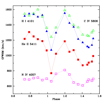
Figure 3: Full width at half maximum intensity measured with Gaussian fits to the line profiles of NIV 4057 (open squares), He II 5411 (filled-in squares), C IV 5806 (open triangles), H I 4201 (filled-in triangles) in the 1999 spectra. All lines except N IV display the sudden decrease in width when star A is “in front” ($\phi\sim$0). A more gradual decrease is observed at the opposite eclipse ($\phi\sim$0.36). This is the same behavior seen in the late 1970’s. The dotted line connects the data points. Data at eclipse phases correspond to the renormalized spectra.

The change in full-width at half maximum (FWHM) is illustrated in Figure 3 obtained from the Gaussian function fits to HI (+He II) 4101, N IV 4057, He II 5411, and CIV 5806/12 Å as a function of orbital phase, showing that different lines behave differently. However, the qualitative nature of the variations we observe in 1999 is as reported in previous optical observations (Moffat et al. 1998; Breysacher et al. 1980; Breysacher 2000). This effect is only one aspect of a much more complex phase-dependent line profile variability pattern that involves asymmetric distortions in the line shape. Thus, the amplitude of any RV curve derived from the emission lines depends on how the lines are measured; that is, it depends on where within the system the emission lines are assumed to originate.

Fortunately, optical and UV spectroscopic monitoring of HD 5980 since the late 1970’s provides the first of three pieces of solid information to aid in interpreting the variability: numerous emission lines that are currently present in the spectrum were absent prior to the early 1980’s. The RV variations of the “new” lines indicate that they arise in star A. This is also true of the “new” UV lines observed with IUE and HST (Koenigsberger 2004 and references therein).

A second fact is that lines arising primarily in the inner portions of the stellar wind are less susceptible to distortions due to wind-wind interaction effects than lines that arise from outer wind regions. The former tend to originate from atomic transitions between excited states, and from elements of lower chemical abundance and are visible only because the density of the inner, accelerating portions of the wind is sufficiently large. Hence, lines from abundant ions and having large transition probabilities, such as H$\alpha+$He II 6560 Å and He II 4686 Å should be avoided during the RV curve analyses, while lines such as N IV 4057 Å may better describe the orbital motion.

The third datum that aids in the interpretation of the lpv’s is that the system is eclipsing and the largest RV’s occur near orbital phase $\phi=$0.15. In addition, due to the geometry of the orbit, during the eclipse at $\phi=$0.00 only the wind of star A contributes emission or absorption at wavelengths shorter than the rest wavelength.

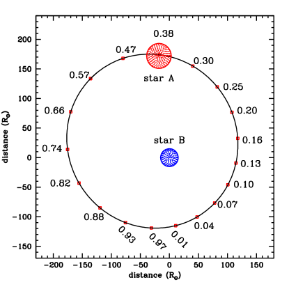
Figure 4: Schematic representation of the orbit indicating orbital phases in a frame of references in which star B is at the origin. For this representation, the masses M${}_{A}=$70 M_⊙ and M${}_{B}=$54 M_⊙ (see Section 4), and the eccentricity and argument of periastron are, respectively, e=0.3 and $\omega=$133^∘; and R${}_{A}=$21 R_⊙, R${}_{A}=$15 R_⊙ from BP91. The observer is located off the page at the bottom of the figure.

Figure 4 provides a guide to the location of star A with respect to star B (located at the center of this coordinate system) as seen by an observer located at the bottom of the page. The red squares that are labeled with the orbital phases correspond to the location of star A at that given time. Periastron passage occurs near $\phi=$0.07.

0.3.1 Emission lines

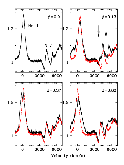
Figure 5: Line profiles at $\phi=$0.0 (top left) used as a template to compare with profiles at $\phi=$0.13 (top right), 0.37 (bottom left), and 0.80 (bottom right). The template is shifted by +275 km/s (top panel, right) and -150 km/s (bottom panel, right). Spectra at $\phi=$0.0 and 0.37 are renormalized to account for the eclipses. The arrows point to excess emission that appears to be associated with star B. The velocity scale is centered on the He II $\lambda_{0}=$4541.59 line, corrected for SMC motion ($+$150 km/s).

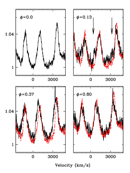
Figure 6: Same as previous figure, but for 3 of the He II lines in the 6000-6200 Å region. V=0 km/s corresponds to $\lambda_{0}=$6100. Å.

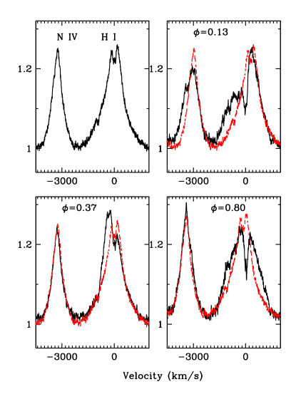
Figure 7: Same as previous figure, but for N IV 4057 and H I 4100 Å. Velocity scale is centered on $\lambda$ 4101.73 Å.

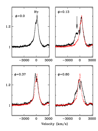
Figure 8: Same as previous figure, but for H$\gamma$.Velocity scale is centered on $\lambda$ 4340.45 Å.

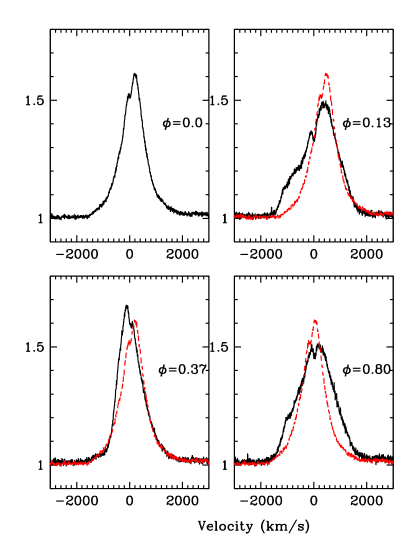
Figure 9: Same as previous figure, but for He II 5411 Å. Velocity scale is centered on $\lambda$ 5411.52 Å.

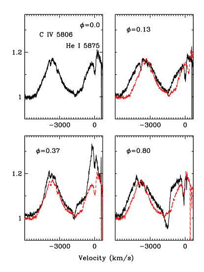
Figure 10: Same as previous figure, but for He I 5875.80 Å.

With the above ideas in mind, we compared the 2005 FEROS line profiles obtained at orbital phases 0.13, 0.36 and 0.80 with the profiles observed at $\phi=$0.00. The spectrum at $\phi=$0.0 is expected to be dominated by star A emission. The individual line profiles are illustrated in Figures 5–10, plotted on a velocity scale corrected for a SMC motion of $+$150 km/s. The top left panel contains the $\phi=$0 spectrum. The other three orbital phases are presented in the remaining panels, and compared with the $\phi=$0 profile, which has been shifted in velocity scale to align major features. For example, Figure 5 displays the He II 4542, N V 4603 and N V 4621 Å lines. The velocity shift required to align the maxima of the three emission lines at $\phi=$0.13 is $+$275 km/s, while for $\phi=$0.8, the He II 4542 Å emissions are aligned with a shift of $-$150 km/s.

We first consider the profiles of N V 4603, 4621 (Figure 5) and the weak He II lines in the $\lambda\lambda$6000–6200 Å region (Figure 6). At $\phi=$0.13 excess emission is apparent in the blue emission line wings, pointed out by arrows. In N V 4603, 4621 Å it can be seen as narrow sub-peaks that “fill in” the P Cygni absorption components. A similar excess emission at this phase appears in N IV 4057, H$\delta$ (Figure 7), H$\gamma$ (Figure 8), He II 5411 (Figure 9) and C IV 5806-11 (Figure 10). We interpret this excess blue emission as emission arising in star B, which is approaching the observer at $\phi=$0.13.

No relative shift was applied to the spectra at $\phi=$0.37 since the N IV 4057 line coincides almost exactly with the profile of $\phi=$0. In most of the other lines, at least the red wings match very well, but blueward of line center one can easily see that excess emission is present.

At $\phi=$0.8 the lines present two different patterns. In the first, N IV 4057, the weak He II 6000-6200 Å emissions and the N V 4603 P Cygni absorptions match the shifted $\phi=$0 line profiles. Thus, these features are primarily formed in star A and have negative RV’s due to its approaching orbital motion. The second pattern, however, is more prevalent and consists of the presence of excess emissions on both wings, although the excess red emission is generally more extended than the blue. Within the context of the interpretation given above, the excess red emission at $\phi=$0.8 originates in star B, which is receding from the observer at this phase. The excess blue emission, however, appears to arise from an additional source. It is tempting to suggest that it arises from the same source as that which produces excess emission at $\phi=$0.36, although its projected velocity towards the observer is greater at $\phi=$0.8 than at $\phi=$0.36.

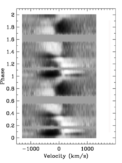
Figure 11: Grey scale representation of residuals for N IV 4057. Phase increases from the bottom to the top, the same data being plotted twice. White corresponds to positive residuals, black to negative. Residuals are the difference between the nearly equally-spaced (in phase) 1999 FEROS spectra and the average of these same spectra. Gaps in phase coverage are filled in with grey background color.

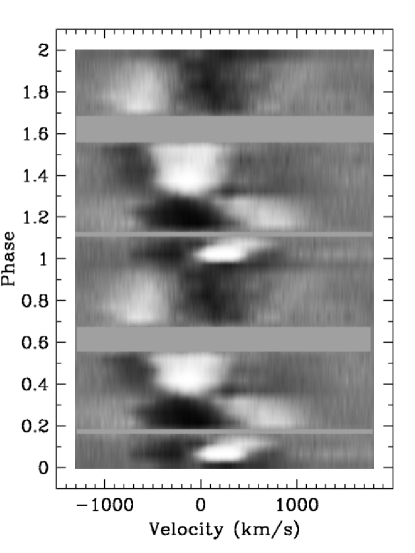
Figure 12: Grey scale representation of 1999 FEROS data for He II 5411 as in previous figure

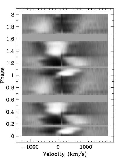
Figure 13: Grey scale representation of 1999 FEROS data for H$\beta$+He II as in previous figure.

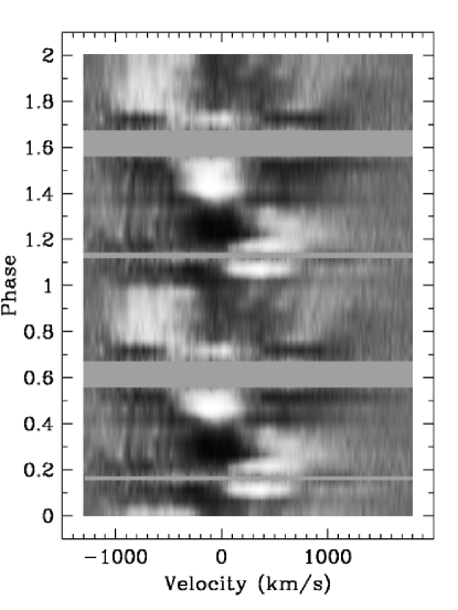
Figure 14: Grey scale representation of 1999 FEROS data for HeI 6678 as in previous figure.

Figures 11–14 are grey-scale representation of the 1999 FEROS data and provide a global view of the lpv’s in 4 representative lines: N IV 4057, He II 5411, H$\beta$+He II 4860 and He I 6678 ÅṪhey are constructed with line profile residuals, stacked from bottom to top with increasing orbital phase. The residuals are the difference between each individual spectrum and the average of the 15 spectra obtained over a single orbital cycle and listed in Table 2 (the first two spectra of this table were not included here). The spacing between the spectra is $\Delta\phi\sim$0.05 in orbital phase, and to consistently retain this spacing in the dynamic plots, the gaps of missing phase coverage are filled-in with grey background color. Plotting the same data twice provides a clearer picture of the orbital-phase dependent trends. The white regions in these images correspond to excess emission; the black to emission deficiency with respect to the mean, or absorption. The maximum dynamic range is typically 10–15% in the residuals with respect to the normalized mean profiles.

All four dynamic plots display similar large-scale trends, specifically, the excess emission traces out a curve suggestive of orbital motion associated with star A. Some of the details of the plots, however, are different. For example, there is a fainter sinusoidal curve that moves in anti-phase with the more dominant bright sinusoid that is clearly seen in He I 6678 and H$\beta$+He II 4860, weaker in He II 5411, but not detectable in N IV 4057. In He I 6678, this secondary curve has a ”whisp-like” structure around $\phi=$0 in the velocity range 0 – 1000 km/s. A striking difference between N IV 4057 and H I 6678 is the very extended blue emission in the phase interval $\sim$0.9–1.0 in the latter. While N IV 4057 shows a rapid shift towards the red, as expected from the orbital motion of star A, He I 6678 stays very much the same, extending over the velocity range $-$300 to $-$1100 km/s. This implies the presence of emitting gas that is approaching the observer with a speed that is not correlated with the orbital motion within this phase interval.

0.3.2 Peculiar behavior of He I P Cygni absorptions

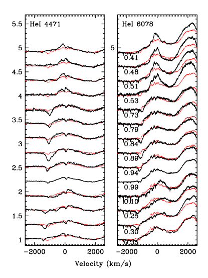
Figure 16: Montage of the 1999 individual FEROS spectra obtained over a single orbital cycle illustrating the behavior of the He I P Cygni absorption components. The template (dotted spectrum) is the profile at $\phi=$0.99, renormalized to account for the eclipse. The spectrum at $\phi=$0.35 is also renormalized. The absorption is strong during the phase interval $\phi=$0.73-0.30, but nearly vanishes at $\phi=$0.99 (eclipse of star B). The y-axis is relative intensity, each spectrum having been shifted along this axis by 0.3 units. The x-axis is velocity with respect to the laboratory wavelength, corrected for SMC systemic motion (+150 km/s).

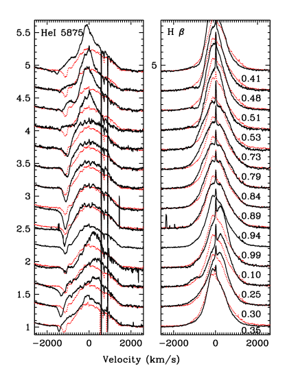
Figure 17: Same as previous figure, but for He I 5875 Å (left). The same behavior is observed for the P Cygni absorptions. Note that when they are sharpest and strongest, the emission component has a very rounded shape. When the P Cygni absorption is not as prominent, the emission appears to have a sharper (possibly superposed) additional emission component. The right panel illustrates the same montage of spectra at H$\beta$. The y-axis is relative intensity, each spectrum having been shifted along this axis by 0.3 units. The x-axis is velocity with respect to the laboratory wavelength, corrected for SMC systemic motion (+150 km/s).

A clue to the origin of the excess blue emission at $\phi=$0.80 may lie in the behavior of the He I lines. As an example, consider the blue wing of He I 5875 Å that is shown in Figure 10. At $\phi=$0.80, a sharp P Cygni absorption is present in the same velocity range as the excess blue emission in the H I and He II lines shown in the grey-scale plots discussed above. Such sharp and strong P Cygni absorptions are usually associated with lines that are formed far from the star, in the low-density regions that are expanding at a constant speed, usually the terminal wind speed, v_∞. The presence of the absorption would not be surprising were it not for its absence or weakness at other orbital phases. This effect can be more clearly appreciated in Figures 15, which displays montages of He I 4471, 5875, 6678 and 7965 Å at the four orbital phases $\phi=$0.0, 0.13, 0.37 and 0.80, and in Figures 16 and 17 where the fuller orbital phase coverage of the 1999 data shows that the absorptions are strongest in the orbital phase interval 0.7–0.9. They nearly vanish at $\phi\sim$0–0.10 (around periastron passage), and re-appear briefly right before the secondary eclipse at $\phi=$0.36. They are then very weak or absent (or greatly displaced) between $\phi=$0.36 and $\sim$0.7.

There is no immediate explanation for this behavior, although similar features as described here have been linked to the WWI interface in the well-documented case of V444 Cygni (Marchenko et al. 1994, 1997), GP Cep (Demers et al. 2002), $\gamma^{2}$ Vel (De Marco, O., 2002), and $\eta$ Carinae (Nielsen et al. 2007). It is also interesting to note that in these four systems the observations lead to the conclusion that there are substantial differences in strengths and velocities of the leading/trailing WWC arms. A similar scenario for HD 5980 will be discussed in Section 8.

In summary, we find that the only lines in the optical spectrum of HD 5980 that are likely to truly describe the orbital motion of star A are N IV 4057, N V 4603 and some of the weak He II lines in the $\lambda\lambda$6000–6200 Å range.

0.4 New constraints on the masses of the system

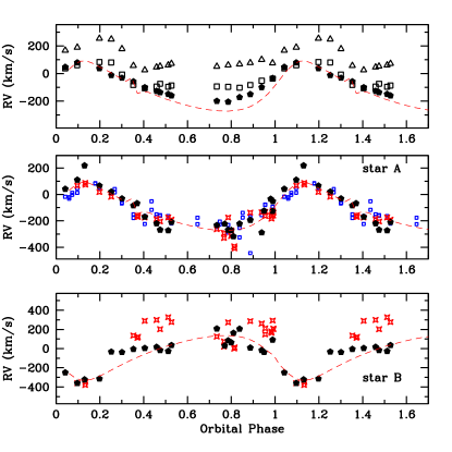
Figure 18: Radial velocity measurements. Top: A single Gaussian was fit to lines of N IV 4057 Å (filled pentagons), H I 4101 Å (squares) and He II 5411 Å (triangles). Each RV curve has a different shape due to contributions from different sources. Middle: Star A’s contribution isolated using a 2-function fit to N IV 4057 Å (filled pentagons) and N V 4603 Å (stars), and a single Gaussian to He II 6074 and 6118 Å (small squares). Arbitrary vertical shifts were applied to correct for different zero-point locations and align the 4 RV curves. Bottom: Star B’s deduced contribution derived from the 2-function fit to N IV 4057 Å (filled pentagons) and N IV 4603 Å (stars). The dashed curves are theoretical computations for a 70$+$54 M_⊙ binary system in an e$=$0.3, $\omega=$133^∘ orbit. All RVs are corrected for the SMC systemic velocity (+150 km/s).

The top panel of Figure 18 illustrates the RV curves that result when the centroid of the emission lines is measured using a single Gaussian fit. The corresponding data are listed in columns 4, 7 and 10 of Tables 2 and 3. The RV curve for N IV 4057 Å line is very similar to that derived by Barbá et al. (1997), indicating that star A is still the major contributor to this line. The H I $+$ He II 4101 and He II 5411 Å display a similar trend, but with different amplitudes and shapes, implying that they contain a more significant contribution from star B and from the WWI region.

Assuming that the line profile variability is in part due to the superposition of emission arising in two distinct sources, we deblended the lines using a two-function fit to the profiles. The results of these measurements are plotted in the middle and bottom panels of Figure 18 (filled-in pentagons), showing two RV curves in anti-phase. Using a similar procedure, we deblended the N V 4603 emission (open stars) using two Gaussians. The results for N V are more uncertain for two reasons: 1) the P Cygni absorption component of the neighboring N V 4621 Å line limits the extent of the N V 4603 Å red wing; 2) at $\phi=$0.13, star B’s component is shifted into star A’s P Cygni absorption component. On some spectra, this superposition makes it very difficult to measure the secondary component, since it simply fills in the P Cyg absorption but is not prominent enough to enter the two-function fit. Because star A’s contribution is dominant, its RV curve is not severely affected by these two effects. However, that of star B not only displays much larger scatter, but also a systematic deviation from the RV curve derived from N IV 4057. Part of this deviation may also be due to NV emission arising in the WWI region.

The middle panel of Figure 18 also contains the RV variations of the weak He II 6074.1 and He II 6118.2 Å lines (small open squares), obtained by fitting a single Gaussian function. These lines show a slightly smaller RV amplitude than that of N IV 4057 Å  consistent with the notion that they arise primarily in the wind of star A but also contain a contribution from star B.

The shape of the RV curve of star B shown in the bottom panel of Figure 18 matches quite well the mirror of the RV curve for star A, within a constant factor (related to the relative masses of the 2 stars), thus supporting the hypothesis that the excess emission (with respect to the $\phi=$0 spectrum) is in fact primarily coming from the 2 stars. The WWI excess should be out of phase with the orbital motion.

We performed a fit to the RV amplitude of NIV and NV using the genetic algorithm PIKAIA (Charbonneau, 1995). The radial velocity curves of the two stars were fitted simultaneously, giving the two RV semi-amplitudes (K1 and K2), the eccentricity $e$, and the longitude of the periastron $\omega_{per}$. The semi-amplitudes are K${}_{A}=$198 km/s (NIV) and 180 km/s (NV), and K${}_{B}=$222 km/s from both lines. These results lead to $M_{A}=$58–79 M_⊙ and $M_{B}=$51–67 M_⊙, adopting an orbital inclination angle $i=$88^∘ (Moffat et al. 1998), and given the uncertainties in the fit to the RV curves ($\pm$4 km/s and $\pm$16 km/s for star A and star B, respectively). The corresponding range in semimajor axis is $a=$143–157 R_⊙. The orbital eccentricity derived from both N IV and NV solutions is $e=$0.30$\pm$0.16. This value is compatible with $e=$0.27 (Moffat et al. 1998) and $e=$0.32 (PB91). The longitude of periastron that we derive lies in the range $\omega_{per}=$283^∘–294^∘. This is smaller than the corresponding values of $\omega_{per}=$319${}^{\circ}\pm$6 (Moffat et al. 1998) and $\omega_{per}=$313^∘ (BP91). Given that the RV curve has a limited orbital phase coverage and that various interaction effects are present in the emission-line spectrum, we favor the values of $\omega_{per}$ derived from the photometric light curve and polarimetry (BP91 and Moffat et al. 1998).

The above masses are significantly larger than those based on single function fits to the emission lines and they are more consistent with the stars’ position on the H-R Diagram near the 120 M_⊙ evolutionary track (Koenigsberger 2004).

0.5 Declining wind densities ?

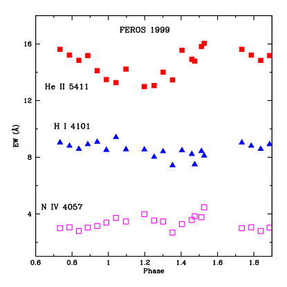
Figure 19: The equivalent width of 1999 FEROS data as a function of orbital phase for N IV 4057 Å  H$\delta+$ He II 4101 Å and He II 5411 Å.

The emission lines in 2005 are substantially weaker than observed in 1999, indicating that the trend for decreasing wind densities that was observed in UV spectra (Koenigsberger 2004) is continuing. In order to quantify the effect, we measured the equivalent width (EW) of H $\delta+$HeII 4101 Å  NIV 4057 Å  and He II 5411 Å as listed in Tables 2 and 3. The orbital phase-dependent variability in 1999 is plotted in Figure 19, showing that He II 5411 Å displays a large modulation with a broad minimum centered around $\phi\sim$0.15, while N IV 4057 Å gives only a hint of an eclipse at $\phi=$0.36. No clear phase-dependent changes are evident in H$\delta+$He II 4101 ÅḞigure 20 illustrates the ratio EW(He II 5411)/EW(H$\delta+$He II 4101) as a function of orbital phase for the two different epochs, 1999 and 2005, leading to the conclusion that the degree of ionization in HD 5980 is greater in 2005 than in 1999. Consistent with this conclusion is the significanly weaker N III 4640 Å blend in 2005 compared to that of 1999.

Hence, these are indications that HD 5980’s wind is reverting to its state prior to the 1993/1994 eruptions, when the emission lines were much broader and significantly weaker (Koenigsberger et al. 1998a; Moffat et al. 1998).

0.6 Stationary photospheric absorptions

A striking feature in the 2005 FEROS data is the strength of photospheric absorptions clearly seen superposed on the emission lines (see, for example, Figures 2, 7, 8, 10, and 15). Similar absorptions have been observed in 1999 HST/STIS spectra (Koenigsberger et al. 2003), and found to be relatively stable in wavelength; that is, the amplitude of the RV variations was $\leq$40 km/s, which was within the uncertainties of the RV measurements. Table 5 lists the dominant absorption lines that we identified in the 2005 FEROS data, with measurements of their RV (columns 2,4,6, and 8) and their corresponding FWHM (columns 3, 5, 7, and 9), measured with Gaussian fits to the profiles. It is important to note that since these features are superposed on strongly variable emission lines, the extent of the absorption line wings is nearly impossible to establish. Hence, the RV measurements refer to the line cores and these do not display any significant RV variations. In fact, if we average the RV values for each orbital phase listed in Table 5, we find that the average RV values are virtually constant, within the standard deviation of the measurements at each orbital phase. The averages and standard deviations are listed in the bottom rows of Table 5. The average velocity at each of the 4 orbital phases listed in this table are within the range 161–172 km/s, with a corresponding range in standard deviations of $\pm$16 – $\pm$22 km/s. Hence, they are indeed stationary within the timescale of the 2005 observations.

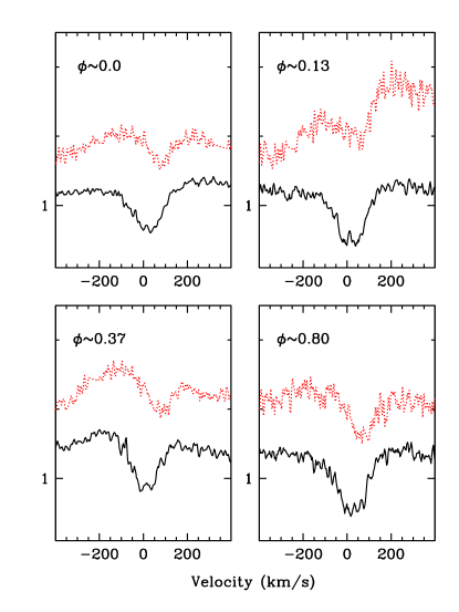
Figure 21: Comparison of the He I 4471 Å photospheric absorption line in the 1999 (dotted) and in 2005 at four orbital phases. The velocity scale is corrected for an assumed SMC systemic velocity of $+$150 km/s, and the 1999 data were shifted upward for clarity in the figure. Note that the 2005 profiles are blue-shifted and stronger than the 1999 profiles. The 1999 spectra were obtained over the timescale MJD 51381.4-51391.4.

The photospheric absorptions are believed to arise in star C (Niemela, 1988; Koenigsberger et al. 2001) which is a reasonable conclusion, given their apparently stationary nature over the P=19.2654 day orbital timescales. Over longer timescales, however, the RV and strength of the lines undergo changes, as illustrated in Figure 21, where the He I 4471 Å lines observed in 1999 and 2005 are compared. At each of the four orbital phases plotted in the figure, the 1999 profiles are significantly redshifted with respect to those of 2005. Schweickhardt (2000) measured the RVs of the O III 5592.4 photospheric absorption line in 1999 FEROS data, finding them to be periodic with P${}_{starC}\sim$96.5 days, and suggested that star C is itself a binary system. His analysis of the RV curve implies that the star C system is very eccentric ($e=$0.83; $\omega=$255^∘; T${}_{0}=$2451183.6) and that the amplitude of the star responsible for the O III photospheric absorption is $K=$71 km/s. Similar results were derived from the analysis of the He I 4471 Å photospheric absorption. Our 2005 data only cover a fraction of the phase for such a period, $\phi_{starC}\sim$0.4–0.8, which lies in a relatively constant portion of the star C RV curve. However, OIII 5592.4 RV variations do show a declining trend with total amplitude of $\sim$20 km/s which is consistent with Schweickhardt’s (2000) conclusion. If this binary is gravitationally bound to the A$+$B pair or whether it is merely a line-of-sight projection remains to be resolved. In any case, however, Schweickhardt’s (2000) results suggest that star C is also an intriguing object that requires further analysis.

An explanation for why the photospheric absorption lines appear to be more prominent in 2005 compared with 1999 may lie in the decreasing visual brightness of star A which thereby makes star C’s photospheric absorptions appear more prominent. Another possibility is that since the emission lines became weaker in 2005 compared with 1999, photospheric absorptions from star A could enhance the strength of absorptions in the combined spectrum.

In Table 5 we have also listed the measurements of a photospheric-like dip observed at orbital phase $\phi=$0.13 “blue-ward” of the stationary absorptions. It is typically located $-$500 km/s from the stationary absorptions, with a FWHM$\sim$500 km/s. At this phase, star B is approaching the observer and it is conceivable that these broad features could be associated with its photospheric absorptions. The large width and the excess blue-shift (with respect to the orbital motion) could be produced by the velocity gradient in its photosphere. An alternative explanation may reside in the presence of a slower-moving wind region (or WWI region ?) projected upon the stars at this phase. However, this issue must await further observations since, as the intensity of the emission lines from star A diminishes, the characteristics of photospheric absorptions will become easier to establish.

0.7 Light curve

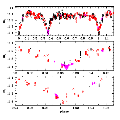
Figure 22: Visual magnitudes from SMARTS (open squares) and Swope (plus signs) compared with differential photometric observations of Breysacher & Perrier (1980; data of July-October 1979) $+$10.415 mag (crosses); and Danish data $+$12.57 mag (filled-in triangles). Orbital phases for the Danish2005, SMARTS and Swope data sets were computed using T${}_{0}=$JD2443158.705 and P=19.2654 days from Sterken & Breysacher (1997). The orbital phases of BP80 data are as listed in their Table 1, which BP80 computed with T${}_{BP80}=$JD2443158.771 and P${}_{BP80}=$19.266 days. The difference in phase computed with P and P_BP80 is $<$0.002 for the BP80 data.

Figure 22 illustrates four sets of HD 5980 photometry. The best full orbital phase coverage (open squares) consists of visual magnitude observations obtained using the CTIO/SMARTS telescope during 2005. The second set having full phase coverage consists of the original Breysacher & Perrier (1980) differential magnitudes (crosses), with a constant value of 10.415 mag added in to make the average levels coincide with those of the SMARTS and the Swope data at orbital phase 0.60. The Swope data (small plus signs) has a poorer overall phase coverage, but covers portions of the ascending branch of the $\phi=$0.36 eclipse more densely. Finally, the Danish telescope differential magnitudes to which the constant value of 12.57 mag has been added (triangles) are primarily concentrated around $\phi=$0.99 and around the $\phi=$0.36 eclipse phase. The top panel of Figure 22 illustrates the complete light curve, while the middle and lower panels focus on the two eclipses.

The difference between the 2003 (SWOPE) and 2005 SMARTS data sets during the ascending branches of both eclipses (there is practically no 2003 data during the descending branches) is noteworthy. It shows the large degree of epoch-to-epoch variability in the system. Also, we should note that in order to shift the photometric minimum to the anticipated $\phi=0.36$, a slightly corrected $T_{modified}=$2443158.865 is suggested, which also better accomodates the photometry obtained in 1994-1995 (Moffat et al. 1998). This implies a significantly larger difference with respect to the Sterken & Breysacher (1997) T${}_{0}=$2443158.707$\pm$0.07 than their quoted uncertainty. The possibility that this shift is related to apsidal motion and a full analysis of the eclipse light curve will be explored in a forthcoming investigation. It is important to note that the analysis requires a methodology as that used by Breysacher & Perrier (1991) in which the extended nature of the continuum eclipsing sources is contemplated.

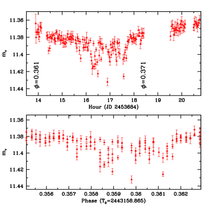
Figure 23: Differential photometric observations from the Danish telescope at $\phi=$0.36–0.37, after adding +12.57 mag to convert to visual magnitudes consistent with the SMARTS values. Top: plotted as a function of time (in hours). Bottom: plotted as a function of orbital phase, using P=19.2654 d and T${}_{modified}=$JD2443158.865. With this T_modified, the secondary minimum is centered on $\phi=$0.36. The error bars correspond to the uncertainty per individual data point, $\sigma_{instr}$.

The longest train of Danish data was obtained around eclipse at $\phi=$0.36–0.37, and the individual data points are plotted in Figure 23, disclosing $\sim$0.^mag035 amplitude variations within a timespan of half an hour. This is considerably shorter than the $\sim$6-hour periodic variations (0.02 mag) reported by Sterken & Breysacher (1997) and attributed to oscillations of star A. Curiously, if we assume T${}_{0}=$T${}_{modified}=$JD 2443158.865, then the two prominent minima appear symmetrically located around $\phi_{modified}=$0.36 (where $\phi_{modified}$ is the phase computed using the modified value of T₀). This would seem to indicate the presence of a bright emitting source that is eclipsed just prior to and just after mid-eclipse, but not during mid-eclipse. Or, alternatively, the presence of dense, eclipsing gas located at a distance from star B that is slightly larger than the radius of star A. One geometry for such a gas that comes to mind is that of a WWI interacting region whose apex is transparent to optical radiation.

Strong variability near $\phi=$0.36 on similar timescales has previously been reported in polarimetric observations (Villar-Sbaffi et al. 2003), and two HST/STIS UV observations obtained one day apart at these same phases suggest that the wind speeds are very variable.

0.8 The wind-wind interaction region

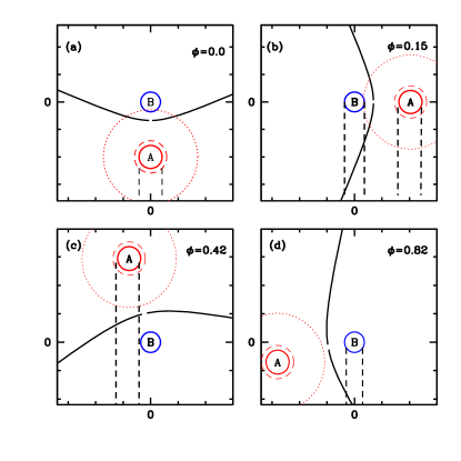
Figure 24: Cartoon of the system geometry for different orbital phases, illustrating how the lines-of-sight to the two stars cross different portions of the WWI region and the stellar winds. Dashed lines contain the columns of gas projected onto the continuum-emitting regions, as seen by an observer situated at the bottom of the page. Discontinuous circles around star A indicate the accelerating portion of the wind (1.5R_A) and the assumed extent of a line-emitting region ($\sim$4R_A).

The current view of the HD 5980 system, consisting of two stars with powerful winds, implies the presence of an interaction zone. Thus, at least part of the variability reported in this paper may result from phase-locked wind-wind interaction effects. In its simplest representation, the WWI region can be modeled in terms of a discontinuity between the two winds that consists of the two thin shocks formed when the supersonic winds collide and whose shape depends on the momentum ratio of the stellar winds. Figure 24 is a cartoon illustrating the WWI region shape for HD 5980, assuming that the wind of star A dominates. This assumption is based on the fact that all emission lines in the combined spectrum increased significantly in strength after the 1994 eruption and that the phase of their Doppler motions corresponds to that of star A (Koenigsberger 2004). The significantly larger emission measure from star A compared to star B is expected to correlate with a larger density. Preliminary stellar wind models for the HD 5980 system that have been fit to FUSE 2002 data imply that star A’s mass-loss rate was still large, $\dot{M}_{A}\sim$10^-4 M_⊙/yr (Georgiev et al., in preparation). In addition, for star B, Moffat et al. (1998) found $\dot{M}_{B}=$2$\times$10^-5 M_⊙/yr from polarimetric data obtained prior to the eruption. These mass-loss rates, combined with wind terminal speeds derived from UV and FUV observations lead to the WWI shock cone configuration shown in Figure 24, with a shock cone opening angle $\sim$50^∘.

Four orbital phases are shown. Star A is represented with three concentric circles depicting, respectively, its photosphere (R_A), the extent of its accelerating wind region in the case of a “fast” velocity law ($\sim$1.5 R_A), and the extent of the dominant emitting wind region for a moderately strong, but arbitrary, emission line ($\sim$4 R_A). Note that because the orbit is eccentric, the WWI discontinuity intersects the line emitting region around periastron passage, but not around apastron. When the WWI region intersects the line-emitting region, the intensity of the observed line-profile is truncated at the corresponding velocity range. The sets of dashed lines drawn parallel to the line-of-sight in Figure 24 enclose columns of wind material that are projected against the luminous stellar continua and that are expanding towards the observer (located at the bottom of the figure). All P Cygni absorption components observed in the spectrum arise in these columns.

The behavior of the blue-shifted, sharp absorption components of the He I emission lines suggests that they arise in the WWI region. They are strongest during the orbital phase interval 0.7–0.9 (when both stars are in view and one of the WWI arms lies in the foreground of star B) and they are weak at $\phi\sim$0–0.10 (when mostly star A is in view) and $\phi=$0.36 – 0.7 (when mostly star B is in view). It is important to note that the sharp and deepest portion of the P Cygni absorption components generally arise in the wind regions that have attained terminal speeds. In the 1999 data, at orbital phase $\sim$0.8, the He I 4471 Å sharp feature extends between -900 to -1340 km/s, and maximum absorption at $\sim-$1130 km/s (assuming a correction for SMC motion of $-$150 km/s). This is significantly slower than terminal wind speed of $-$1750 km/s inferred for star A during the same epoch from HST/STIS observations of UV lines (Koenigsberger et al. 2000). This slower speed is qualitatively consistent with absorption of star B radiation traversing the foreground WWI region arm. Also noteworthy is the fact that excess blue-shifted emission appears in many lines around orbital phase $\phi=$0.36, which is tempting to attribute to emission arising in the WWI zone that is not projected against either continuum source.

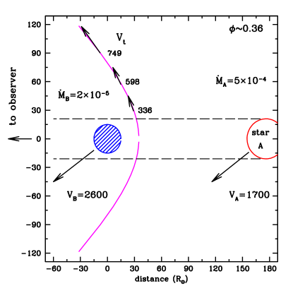
Figure 25: Schematic representation of the WWC shock cone at orbital phase 0.36 listing tangential flow velocities (v_t) computed using the relations given by Cantó et al. (1996). The assumed mass-loss rates are in M_⊙/year and velocities are in km/s. The observer is off the page to the left at $\phi=$0.36. The dashed lines contain the column of material traversed by the line-of-sight from the observer to star A. With the assumed radii (R${}_{A}=$15 R_⊙ and R${}_{B}=$21 R_⊙), the light from star A’s disk must pass through the WWI region and star B’s inner wind before reaching the observer. Time-dependent mass ejections from star B or instabilities along the WWI region could be responsible for the rapid variability observed at this orbital phase.

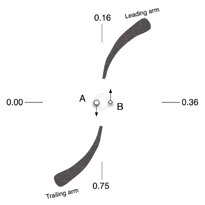
Figure 26: Cartoon illustrating an alternative geometry for the WWI region that would be consistent with the orbital phase-dependent behavior of the He I P Cygni absorption components.

Figure 25 provides estimates of the flow velocities, V_t, along the shock cone walls derived from the expressions given by Cantó et al. (1996), using the roughly estimated values for mass-loss rates of the two stars. At orbital phases around 0.8, the line-of-sight from the observer to star B crosses regions of the WWI having V${}_{t}\sim$600–800 km/s. Considering that the shock cone has an opening angle $\sim$50^∘, the maximum projected speed of V_t along the line-of-sight in the stationary frame of reference is $\sim-$600 km/s. This is significantly smaller than the speeds at which the He I P Cygni absorption components are being observed. Correcting for the orbital motion of star B of $\sim$220 km/s brings the predicted value closer to the observations at $\phi\sim$0.15, when star B is approaching the observer, but increases the discrepancy round $\phi\sim$0.8. However, the idealized WWI model presented in Figures 24 and 25 is a greatly simplified model. For example, if we take into account that the axis of symmetry for the WWI shock cone is in reality tilted with respect to the line connecting the two stars, the angle between the leading WWI arm and the line-of-sight decreases, allowing for faster projected speeds. In addition, numerical simulations that include orbital motion show that the shock cone arms are curved. Hence, the leading and the trailing arms could cross the line-of-sight to the stars at at different orbital phases and with larger projected speeds than depicted in Figure 25. Figure 26 is a cartoon that illustrates an alternative geometry for the WWI region, based on an interpretation of the variable He I P Cygni absorption lines. It would be interesting to analyze whether the physical mechanisms involved in the WWI can give rise to such a different geometry, compared to the typical conical surfaces that are predicted by the traditional calculations.

It is important to keep in mind that the geometry and characteristics of the interaction region depend on whether the shocked gas is radiative or not, and this, in turn, determines the intensity and shape of line emission/absorption that the WWI region can produce. One can estimate whether the gas is radiative or not using the parameter $\chi$ from Stevens et al. (1992), which is the ratio of the postshock cooling timescale to the flow time out of the system. Hydrodynamical models have indeed confirmed that the postshock gas cools rapidly when $\chi\sim$1.0.

To evaluate $\chi$ we need to determine the pre-shock velocity. $\chi$ is highly dependent on this value ($\propto v^{4}$) so small changes in $v$ make a big change in $\chi$. Using the approximation to the velocity law as in St.Louis et al. (2005),

$$v=v_{0}+(v_{\infty}-v_{0})*(1-R_{*}/r)^{\beta}$$ (1)

with $v_{0}=0.16v_{\infty}$ and $\beta=$2.5.

With such a velocity profile the wind accelerates so slowly that the post-shock gas (from both stars) is always highly radiative, and the Canto et al. (1996) prescription used in Figures 24 and 25 is appropriate. However, if the wind(s) accelerate quicker (eg $\beta=$1) then there is a chance that, for example, star B’s shocked wind is adiabatic near apastron (but strongly cooling at periastron).

The fact that the X-ray emission is apparently harder near phase 0.36 (Nazé et al. 2007) is very suggestive that the maximum pre-shock velocity increases as the stars separate, although it is by no means certain that the winds between the stars bear much relation to the winds from single stars. Indeed, indications exist that at least star A’s wind velocity structure facing the companion differs from that of its opposite hemisphere (Koenigsberger et al. 2006).

Unfortunately there have been very few hydrodynamic calculations of the wind interaction in short period systems like HD 5980 where the acceleration of the winds is taken into account (Iota Ori, Pittard 1998; Sand 1, St-Louis et al. 2005). Antokhin et al. (2004) took a slightly different approach which enabled them to calculate the X-ray emission, but the wind needed to be specified by a beta velocity law and was not calculated self-consistently with inhibition and braking in the way that the other hydro models noted were.

If both winds rapidly cool after being shocked, the postshock region collapses into a dense sheet and the shocks are coincident with the contact discontinuity. It is worth noting that in this case one expects very strong instabilities in the WWI region (specifically the non-linear thin-shell instability - see Stevens et al 1992), which means that the position of the contact discontinuity from the Canto et al. model should be viewed only in a time-averaged sense. This is of course a possible cause of the short-timescale fluctuations that are mentioned in Section 7).

Wind clumping is an additional factor that is absent from the simplified view of WWI regions. Pittard (2007) presents simulation of the effects of clumps in binary systems with adiabatic colliding winds. Although the clumps are likely destroyed quite rapidly in such systems, they create a broader distribution of temperatures within the WWI at any given off-axis distance. This is because the interclump material is heated to higher than average temperatures, while the clumps are initially heated to significantly lower temperatures (the shocks driven into them are slower) - the temperature within shocked clumps is lower than the temperature obtained from the collision of smooth winds by a factor equal to the density contrast of the clump to interclump material. If most of the wind mass is within the clumps this should have observable consequences. The shocked material within the clumps is then heated further by additional weaker shocks and mixing within the WWI. In systems where the wind parameters are such that a WWI formed by smooth winds is not far from being radiative, the presence of higher densities within clumps may be enough for cooling to become important (see Walder & Folini 2002).

0.9 Conclusions

In this paper we present results from spectroscopic and photometric observations of HD 5980 obtained in 1999 and 2003-2005. We first analyze the line-profile variability in the 2005 spectra, concluding that in lines that are formed in the dense, inner wind regions, line-profile-variability may be interpreted mostly in terms of the presence of two emission components, the first belonging to star A (the eruptor) and the second associated with star B (the companion). Assuming that the emission-line profiles can be effectively separated with a two-function fit, we find that the centroids of the two functions are consistent with the orbital motion of the two stars, leading to a new estimate of the masses, M${}_{A}\sim$58–79 M_⊙ and M${}_{B}\sim$51–67 M_⊙. These values are significantly larger than previously derived (Niemela et al. 1997), but still imply that the stars must have lost considerable amounts of mass before reaching their current evolutionary state, given their location on the HRD near 120 M_⊙ ZAMS evolutionary tracks (Koenigsberger 2004). The mechanisms by which such large amounts of mass may have been stripped require detailed examination. In addition, it would be very interesting to get more theoretical insight into their current internal stellar structure and hence, be able to establish their current evolutionary state. As pointed out by Koenigsberger et al. (1998b), if star B is a bona fide WNE remnant of the originally more massive member of the binary, its interior may have already reached a very advanced stage of evolution and, thus, it may be nearing the supernova stage. On the other hand, the significantly larger mass that we have now derived for star B (M${}_{B}\sim$56–67 M_⊙ vs. $\sim$28 M_⊙ as believed previously) suggests that it may not yet have reached the core He burning evolutionary phase. Since star B is believed to be the source of the highly He-enriched WR-spectrum observed in the 1970’s (Breysacher, Moffat & Niemela 1982), the implications for stellar evolution theory of such a massive, He-rich object are potentially very interesting.

Line strengths in the 2005 spectra are significantly weaker than those observed in 1999, consistent with a similar decreasing trend observed in UV lines, and suggesting that the eruptor is reverting to a more quiescent state. The question of whether another activity cycle will start in the near future is an important one, since the timescale for the eruptive events provides an estimate of the total amount of mass that may be lost through this mechanism. In addition, the activity timescale provides a clue to understanding the underlying mechanism responsible for the instability. Continued observations are required to determine the long-term variability pattern.

Visual photometric observations in 2005 provide a light curve covering the entire orbital cycle, as well as a detailed description of the system’s brightness variations during selected orbital phases. In particular, relatively large-amplitude ($\sim$0.035 mag) fluctuations appear around secondary minimum, when star B, the non-erupting star, is “in front”. Continued systematic observational monitoring around this orbital phase would be very valuable because of the strong and rapid variations observed in visual photometry, polarimetry and UV P Cygni line profiles. In addition, the X-ray appears to be greater here than around the opposite eclipse.

The temporal behavior of the P Cygni absorption components of the He I lines is qualitatively consistent with the presence of a denser wind structure folding around star B which we associate with the WWI region. However, the observed speeds are not consistent with the simple models. In particular, the flow speeds are significantly larger than predicted in the radiative shock limit and thus suggest that at least one of the shocks is adiabatic. It is interesting to note that the hemisphere of star A that faces the companion is predicted to be particularly active due to tidal interaction effects (Koenigsberger & Moreno 2007), raising the question of how this activity may affect the structure of the WWI region.

The photospheric absorption lines remain stationary over the 19-day orbital cycle. However, we find a systematic shift of $\sim$20 km/s in their radial velocities observed in 1999 with respect to those observed in 2005. This is consistent with the conclusion of Schweickhardt (2000) that star C, the third source in the combined HD 5980 spectrum, is itself a binary system, with P${}_{starC}\sim$96 days. It is unclear, however, whether the star C system is gravitationally bound to the star A+star B pair with a much longer orbital period. It is a curious fact that the star C orbital period is nearly a factor of 5 longer than the orbital period in the star A+ star B pair, which may indicate that the two systems are physically bound. If this were the case, then the eruptive behavior in HD 5980 could be linked to the gravitational perturbations produced during periastron passages. In this case the orbital period of the star C system around the star A+ star B system would be $>$25 years, since only one large eruption has been seen over the $\sim$40 years that the system has been studied.

In the Appendix we list the SWOPE and SMARTS photometry averages for each day of observation (Tables 7–10). The data presented in this paper will be made publicly available (please contact CF or GK).

• Antokhin, I.I., Owocki, S.P., Brown, J.C. 2004, ApJ, 611, 434.

• Auer, L.H. & Koenigsberger, G. 1994, ApJ, 436, 859

• Barbá R.H., Morrell, N.I., Niemela, V.S., Bosch, G.L., González, J.F., Lapasset, E., Ferrer, O.E., Brandi, E.E., Cellone, S.A., Garcia, B.E., Malaroda,S.M., Levato, O.H., Donzelli, C., Feingstein, C., Rich, M. 1996, RMAACS, 5, 85.

• Barbá R., Niemela V.S., Morrell, N. 1997, in ASP Conf. Ser. 120, Luminous Blue Variables:Massive stars in transition, ed. A. Nota & H. Lamers (San Frnacisco:ASP), 238.

• Bateson, F.M. & Jones, A. 1994, Publ. Var. Star. Sec. R. Astron. Soc. New Zealand, 19.

• Breysacher, J.,François P. 2000, A&A, 361, 231.

• Breysacher, J. & Perrier, C. 1980, A&A 90, 207 (BP80)

• Breysacher, J. & Perrier, C. 1991, in IAU Symp. 143, 143, Wolf Rayet Stars and Interrelations with other Massive Stars in Galaxies, eds. K. van der Hucht & B. Hidayat (Dordrecht: Kluwer), 229 (BP91)

• Breysacher, J., Moffat, A. F. J., & Niemela, V. 1982, ApJ, 257, 116

• Breysacher, J., & Westerlund, B. E. 1978, A&A, 67, 261

• Cantó J., Wilkin, & Raga, A. 1996, ApJ, 469, 729

• Charbonneau, P. 1995, ApJS 101 309

• De Marco, O. 2002, ASPC, 260, 517.

• Demers, H., Moffat, A.F.J, & Marchenko, S.V. 2002, ASPC 260, 563.

• Drissen, L., Crowther, P.A., Smith, L.J., Robert, C., Roy, J.-R., & Hillier, D.J. 2001, ApJ 545, 484.

• Everett, M.E., & Howell, S.B. 2001, PASP, 113, 1428

• Gayley, K. et al. 1997, ApJ 475, 786

• Georgiev, L. & Koenigsberger, G. 2004a, A&A, 423, 267.

• Georgiev, L. & Koenigsberger, G. 2004b, IAU Symp. 215, Stellar Rotation, (ed) Maeder& Eenens, p. 19

• Hoffmann, Stift & Moffat 1978, PASP 90, 101.

• Lührs, S. 1997, PASP 108, 504

• Kaufer, A., Schmid, H.M., Schweickhardt, J., Tubbesing, S. 2002, in “Interacting Winds from Massive Stars”, ASP Conf. Ser. Vol. 260, 489.

• Koenigsberger, G., Auer, L.H., Georgiev,L. and Guinan, E. 1998a, ApJ, 496, 934

• Koenigsberger, G., Peña, M., Schmutz, W. and Ayala, S. 1998b, ApJ, 499, 889

• Koenigsberger, G., Georgiev, L., Barbá, R., Tzvetanov, Z., Walborn, N.R.,Niemela, V., Morrell, N., y Schulte-Ladbeck, R. 2000, ApJ, 542, 428

• Koenigsberger, G. 2004, RMAA, 40, 107

• Koenigsberger, G., Fullerton, A., Massa, D., Auer, L. 2006, AJ, 132, 1527

• Koenigsbeger, G. & Moreno, E. 2007, arXiv0705.1938.

• De Marco, O. 2002, ASP Conf. Ser. 260, 517

• Marchenko, S.V., Moffat, A.F.J. & Koenigsberger, G. 1994, ApJ, 422, 810

• Marchenko, S.V., Moffat, A.F.J., Eenens, P.R.J., Cardona, O., Echevarria, J. Hervieux, Y. 1997, ApJ, 485, 826

• Massey, P., Parker, J.W., Garmany, C.D. 1989, AJ 98, 1305.

• Moffat, A.F.J., Marchenko, S.V., Bartzakos, P., Niemela, V.S., Cerruti, M.A.,Magalhaes, A.M., Balona, L., St.-Louis, N., Seggewiss, W., Lamontagne, R. 1998, ApJ 497, 896

• Nazé, Y., Corcoran, M.F., Koenigsberger, G., Moffat, A.F.J. 2007, ApJLett, 658, 25.

• Nielsen,K.E., Corcoran, M.F., Gull, T.R., Hillier, D.J., Hamaguchi, K., Ivarsson, S., Lindler, D.J. 2007, ApJ 660, 669.

• Niemela, V.S. 1988, ASPCS 1, 381

• Niemela, V.S., Barbá, R.H., Morrell, N.I. and Corti, M. 1997, in ASP Conf Ser. 120, A. Nota and H.J.G.L.M. Lamers (eds), p.222.

• Pittard, J.M. 1998, MNRAS, 300, 479

• Pittard, J.M. 2007, ApJ, 660, L141.

• Schweickhardt, J. 2000, PhD Thesis, Ruprecht-Karls-Universität, Heidelberg.

• Sterken C., Breysacher J. 1997, A&A 328, 269

• Stevens, I.R., Blondin, J.M., Pollock, A.M.T. 1992, ApJ 386, 265.

• Stevens, I.R. 1993, ApJ, 404, 281.

• St.-Louis, N., Moffat, A.F.J., Marchenko, S.V., Pittard, J.M. 2005, ApJ, 628, 953.

• St.-Louis, N., Moffat, A.F.J., Marchenko, S.V., Pittard, J.M., Boisvert, P. 2006, ASPC, 348, 121.

• Villar-Sbaffi, A., Moffat, A.F.J., St.-Louis, N. 2003, ApJ 590,483

• Walder, R. & Folini, D. 2002, ASP Conf. Ser. 260, 595.

4 Parameter 1979-81 1994 1999-2005 $P_{orb}$ (days) 19.2654 $\cdots$ $\cdots$ Orbital inclination (deg) 88m $\cdots$ $\cdots$ a ($R_{\odot}$) 127b $\cdots$ 143–157k e 0.3 $\cdots$ 0.30$\pm 0.16$ k $M_{\rm A}$ (M_⊙) 50b $\cdots$ 58–79k $M_{\rm B}$ (M_⊙) 28b $\cdots$ 51–67k M${}_{V}^{sys}$ (mag) $-$7.3a $-$8.7e $-$7.6h M${}_{V}^{A}$ (mag) $-$6.3 $-$8.6e $-$6.5 M${}_{V}^{B}$ (mag) $-$5.8 $\cdots$ $\cdots$ M${}_{V}^{C}$ (mag) $-$6.1 $\cdots$ $\cdots$ $R_{{\rm A}}$ (R_⊙) 21a $>160$d $\cdots$ $\cdots$ 280g $\cdots$ $R_{{\rm B}}$ (R_⊙) 15a $\cdots$ $\cdots$ $R_{{\rm envB}}$ (R_⊙) 30–40a $\cdots$ $\cdots$ $v_{\infty}^{A}$ (km/s) $\cdots$ 300–1700 1740–2200: $\cdots$ 500g $\cdots$ $v_{\infty}^{B}$ (km/s) 3100: $\cdots$ 2600–3100: $v_{\infty}^{C}$ (km/s) $\cdots$ $\cdots$ 1700:: N[He]/N[H]^aa_Non-LTE $\cdots$ 0.4 e $\cdots$ $\dot{M}_{A}$ (M_⊙/yr) $\cdots$ $10^{-3}$e $\cdots$ $\dot{M}_{B}$ (M_⊙/yr) 2$\times$10^-5m $L_{A}$ (L_⊙) $\cdots$ $3\times 10^{6}$e $\cdots$ $\cdots$ $10^{7}$g $\cdots$ $T_{*}^{A}$ ^∘K 53,000c 21,000d $\cdots$ $\cdots$ 35,500e $\cdots$ Spectrum (Star A) WN3b $B1.5Ia^{+}$d WN6d Spectrum (Star B) WN4b WN4: WN4: Spectrum (Star C) $\cdots$ $\cdots$ O4-6f $\cdots$ $\cdots$ O7I n $V_{rot}^{A}\,sin\leavevmode\nobreak\ i$ (km/s) $\cdots$ $\cdots$ 250::j $V_{rot}^{C}\,sin\leavevmode\nobreak\ i$ (km/s) $\cdots$ $\cdots$ 75i P_orb(C) (days) $\cdots$ $\cdots$ 96.5 s aaAbundance ratio by number (0.63 by mass);  ^aBreysacher & Perrier 1991;  ^bNiemela et al. 1997; ^cAssuming $L_{\rm starA}$ ($L_{\odot}$)=const and $R_{\rm starA}$/$R_{\odot}$=21;  ^dKoenigsberger et al. 1998a;  ^eDecember 30, Koenigsberger et al. 1998b;  ^fKoenigsberger et al. 2000;  ^gDrissen et al. 2001;  ^hS. Duffau, assuming m-M=19.1 mag; ⁱKoenigsberger et al. 2001; ^jGeorgiev & Koenigsberger 2004b; ^k This paper; ^m Moffat et al. 1998;  ⁿ Koenigsberger, Fullerton, Massa & Auer 2006; ^s Schweickhardt, J. 2002.

Table 1: Summary of HD 5980 Estimated Parameters

12 spectrum MJD phase NIV 4057.76 HI 4101.71 HeII 5411.52 RV FW $-$EW RV FW $-$EW RV FW $-$EW km/s km/s Å km/s km/s Å km/s km/s Å 78781 51374.418 0.475 13 685 3.83 76 1105 7.94 203 907 14.79 79411 51375.422 0.527 -10 694 4.46 63 1221 8.99 221 993 16.04 80871 51379.402 0.734 -50 689 2.99 56 1515 9.03 201 1217 15.62 81451 51380.398 0.786 -55 685 3.05 53 1546 8.80 211 1306 15.21 82121 51381.402 0.838 -23 705 2.79 47 1538 8.58 218 1249 14.84 83181 51382.352 0.887 -0.5 711 3.03 66 1505 8.91 227 1213 15.18 83811 51383.355 0.939 50 679 3.14 97 1527 9.08 251 1188 14.11 84511 51384.309 0.989 116 697 3.39 113 1316 8.51 226 1066 13.48 85181 51385.332 0.042 197 663 3.72 187 1072 9.41: 317 769 13.27 85771 51386.391 0.097 229 760 3.46 210 1297 8.55 340 1023 14.22 86321 51388.340 0.198 187 810 3.98 233 1553 8.54 404 1185 12.99 86701 51389.383 0.252 138 752 3.53 230 1424 8.02 399 1049 13.06 87211 51390.328 0.301 118 647 3.46 143 1373 8.41 328 1070 14.01 87751 51391.332 0.353 92 624 2.68 66 1215 7.42 207 946 13.46 88931 51392.328 0.405 49 609 3.28 43 1170 8.48 175 872 15.55 89511 51393.371 0.459 23 658 3.57 55 1118 8.22 195 880 14.91 90131 51394.391 0.512 0.5 671 3.76 54 1136 8.43 210 921 15.82

Table 2: FEROS 1999 data

12 spectrum MJD phase NIV 4057.76 HI 4101.71 HeII 5411.52 RV FW $-$EW RV FW $-$EW RV FW $-$EW km/s km/s Å km/s km/s Å km/s km/s Å 0617801 53538.385 0.799 -29 760 2.56 21 1860 5.82 211 1622 15.33 0617531 53538.404 0.800 -31 756 2.63 12 1903 5.80 221 1643 14.56 0620221 53541.384 0.955 78 800 2.70 136 1692 5.31 278 1454 12.96 0620344 53541.403 0.955 73 810 2.99 120 1608 5.62 291 1497 13.38 0710740 53561.367 0.992 98 745 3.13 141 1409 6.37 281 1099 14.07 0710950 53561.386 0.993 98 729 3.11 143 1395 5.98 284 1068 14.83 0725580 53576.288 0.767 -10 817 2.65 91 2003 5.13 270 1705 15.39 0725630 53576.307 0.767 -3 828 2.76 77 1921 5.82 266 1654 15.03 0921331 53635.000 0.814 -19 936 2.32: 23 1952 4.62 216 1747 15.36 0922990 53635.019 0.815 -2 955 2.36 56 2026 5.57 202 1757 14.99 0925220 53638.253 0.983 118 694 2.75 174 1452 5.11 295 1239 13.38 0925481 53638.272 0.984 113 758 2.54 178 1427 4.97 285 1192 13.24 0928220 53641.153 0.133 249 986 2.46 ?? ?? 4.60 420 1629 13.50 0928161 53641.173 0.134 260 921 2.40 ?? ?? 4.82 420 1627 13.46 1022700 53665.026 0.372 85 657 2.53 16- 1290 5.72 159 1088 15.75 1022731 53665.045 0.374 86 666 2.53 0.1 1288 5.59 153 1048 15.92

Table 3: FEROS 2005 data

3 spectrum MJD phase 0619 53541.389 0.955 0630 53552.429 0.528 0710 53561.400 0.994 0921 53634.999 0.814 0924 53638.238 0.982 0927 53641.176 0.135 1010 53654.110 0.806 1012 53656.164 0.913

Table 4: EMMI data

9 $\phi=$ 0.8 $\phi=$ 0.0 $\phi=$ 0.13 $\phi=$ 0.37 Atomic ID RV FW RV FW RV FW RV FW He I 3819.60 142 175 190 286 – – ?? ?? H 9 3835.38 167 260 170 214 186 224 140 267 – – – – -120 468 He I 3888.64c 208 282 198 207a 163 264 195 201 He I 4026.18 182 178 153 119 154 171 144 127 – – – – -324 554 – – H I 4101.76: 194 265 176 213 157 239 156 221 – – – — -314b 579 – – He II 4199.84d 174 278 176 164 171 176 166 186 – – – – -249 547 – – H I 4340.49 163 220 135 232 141 247 141 185 – – -351 406 – – He I 4387.93 149 276 175 137 188 326 170 189 He I 4471.50: 168 185 167 152 161 158 155 132 He II 4541.59 190 181 192 126 165 137 168 183 -249 545 H I 4861.30 176 287 113: 311 141 257 188 326 He I 4921.93 165 207 173 163 156 166 155 178 He I 5015.68 181 144 179 148 173 160 167 123b He II 5411.52 181 178 197 128 177 141 189 125 – – -142 145 -323 400 – – O III 5592.4 166 150 156 149 168 134 148 117 C IV 5801.3 178 177 203 180 165 141 182 170 C IV 5812.0 177 132 200 117 199 136 – – He I 5875.8 173 220 164 190 162 180 162 160 He I 6678.15 436 181 187 113 122 250 – – – – -145 324 419 151 – – He I 7065.71 150 250 154 199 147 234 141 129 – – – – - 549 569 – – N IV 7111.28 152 93 170 105 129 73 136 74 8 156 – – – – – – N IV 7122.98 277 110 – – – – – – 16 81 – – – – – $<>$ 172 – 173 – 161 – 161 – s.d. $\pm$16 – $\pm$22 – $\pm$19 – $\pm$18 –  ^a filled-in by emission;  ^b very clear  ^c blended with H I 3889.05  ^c blended with N III 4200.

Table 5: Photospheric absorptions 2005

6 $<$MJD$>$ $<$phase$>$ Num. $<$m_v-C$>$ $<\sigma_{instr}>$ s.d. 53561.422 0.995 20 -1.244 0.008 0.014 53562.352 0.043 18 -1.397 0.007 0.008 53564.352 0.147 12 -1.501 0.008 0.006 53568.305 0.352 7 -1.234 0.006 0.003 53576.367 0.771 43 -1.423 0.008 0.006 53684.203 0.368 172 -1.186 0.004 0.013 53685.105 0.415 30 -1.375 0.003 0.004 53687.207 0.524 41 -1.440 0.005 0.007 53689.191 0.627 95 -1.442 0.006 0.006 53693.184 0.834 20 -1.452 0.006 0.007

Table 6: Average differential photometry: Danish telescope

————————

Figure 1: Average $\phi\sim$0 low dispersion spectrum obtained with EMMI in 2005 and rectified. The strongest line in the spectrum is He II 4686 Å. Other lines that are mentioned in the text are labeled with their primary identifications. The same spectrum is amplified in the lower panel, to display more clearly the weaker lines.

Figure 2: H I (+He II) line profiles at H$\alpha$, H$\beta$, H$\gamma$, H$\delta$, H$\epsilon$ and H9 3835 Å from FEROS 2005 data. The spectra are averages for each of the orbital phases $\phi=$0.0, 0.13, 0.37 and 0.80, and the spectra at $\phi=$0.0 and 0.37 are renormalized to account for the corresponding eclipses. The velocity scale is corrected for the +150 km/s systemic velocity of the SMC. Sharp emission spikes, strongest at H$\alpha$, are nebular emission.

Figure 15: FEROS 2005 line profiles of He I 7065, 6678, 5875 and 4471 Å (from top down). The spectra are averages for each of the orbital phases $\phi=$0.0 (top left), 0.13 (top right), 0.37 (bottom left) and 0.80 (bottom right). At $\phi=$0.0 and 0.37 they are renormalized to account for the eclipses. The velocity scale is corrected for the +150 km/s systemic velocity of the SMC. Note that the photospheric absorption lines are stationary. The P Cygni absorptions are particularly prominent at $\phi=$0.80.

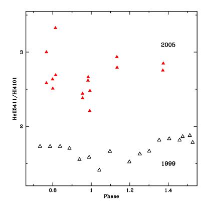
Figure 20: The ratio of equivalent widths of He II 5411 Å and H I (+He II) 4101 Å as a function of orbital phase for the 1999 and 2005 FEROS observations. There is only a hint of an orbital-phase dependence in 1999. Much clearer is the overall change in the ratio from 1999 to 2005, indicating that the degree of ionization increased in 2005.

5 $<MJD>$ $<phase>$ Num. $<m_{v}>$ s.d. 52838.379 0.464 16 11.143 0.017 52839.362 0.515 9 11.154 0.046 52840.324 0.565 12 11.123 0.019 52857.303 0.446 18 11.145 0.012 52858.273 0.497 3 11.122 0.010 52859.257 0.548 5 11.086 0.018 52860.244 0.599 1 11.142 52972.072 0.404 15 11.185 0.006 52973.061 0.455 8 11.110 0.008 52974.059 0.507 16 11.076 0.012 52975.056 0.559 4 11.090 0.005 52991.107 0.392 18 11.236 0.018 52992.063 0.441 19 11.114 0.011 52992.844 0.482 2 11.073 0.001 52993.905 0.537 2 11.038 0.008 53008.062 0.272 7 11.101 0.013 53009.067 0.324 1 11.170 53010.034 0.374 4 11.335 0.013 53011.039 0.426 6 11.180 0.018 53159.403 0.127 4 11.048 0.010 53183.377 0.372 4 11.357 0.016 53210.325 0.771 7 11.117 0.005 53225.305 0.548 7 11.109 0.010 53226.258 0.598 11 11.128 0.011 53227.387 0.656 6 11.154 0.012 53228.295 0.703 6 11.128 0.010 53229.240 0.752 7 11.099 0.016 53230.228 0.804 8 11.135 0.011 53247.271 0.688 7 11.153 0.015 53254.290 0.053 20 11.205 0.013 53288.193 0.812 26 11.137 0.015 53591.385 0.550 2 11.119 0.003 53592.405 0.603 2 11.114 0.003 53593.400 0.655 1 11.120 53596.401 0.810 5 11.122 0.007 53597.378 0.861 1 11.128 53599.223 0.957 2 11.149 0.041 53600.401 0.018 2 11.325 0.006 53602.355 0.119 2 11.084 0.005 53608.313 0.429 2 11.189 0.004 53615.078 0.780 1 11.158 53617.281 0.894 2 11.134 0.006 53618.199 0.942 3 11.138 0.016 53619.232 0.995 1 11.347 53620.238 0.048 1 11.174

Table 7: Average photometric visual magnitudes: SWOPE and SMARTS

5 $<MJD>$ $<phase>$ Num. $<m_{v}>$ s.d. 53621.379 0.107 2 11.091 0.006 53622.366 0.158 2 11.069 0.006 53624.244 0.256 2 11.104 0.008 53625.326 0.312 2 11.191 0.011 53628.267 0.464 2 11.142 0.013 53631.317 0.623 2 11.146 0.004 53632.323 0.675 2 11.145 0.006 53634.303 0.778 2 11.126 0.012 53638.265 0.983 2 11.274 0.008 53640.255 0.087 2 11.137 0.004 53642.245 0.190 2 11.107 0.011 53643.233 0.241 2 11.141 0.014 53646.201 0.395 2 11.288 0.010 53650.388 0.613 2 11.181 0.008 53651.352 0.663 1 11.154 53652.397 0.717 2 11.185 0.003 53655.185 0.862 2 11.101 0.026 53657.186 0.966 2 11.175 0.018 53658.132 0.015 4 11.318 0.016 53660.178 0.121 4 11.070 0.003 53663.209 0.278 2 11.121 0.001 53664.219 0.331 2 11.205 0.004 53665.227 0.383 2 11.329 0.004 53666.232 0.435 2 11.144 0.003 53669.062 0.582 4 11.104 0.006 53670.051 0.633 2 11.121 0.007 53672.047 0.737 1 11.099 53673.020 0.787 3 11.095 0.021 53675.047 0.893 2 11.139 0.002 53676.180 0.951 4 11.158 0.006 53677.196 0.004 2 11.349 0.010 53679.157 0.106 2 11.150 0.007 53680.269 0.164 2 11.100 0.002 53682.075 0.257 4 11.136 0.022 53683.264 0.319 2 11.195 0.011 53685.105 0.415 2 11.186 0.001 53688.131 0.572 2 11.145 0.001 53689.107 0.622 2 11.133 0.000 53691.197 0.731 1 11.225 53692.077 0.777 2 11.159 0.001 53694.082 0.881 2 11.189 0.001 53695.082 0.933 2 11.168 0.008 53698.036 0.086 2 11.082 0.011 53700.083 0.192 2 11.087 0.001 53701.047 0.242 2 11.120 0.002 53703.075 0.347 2 11.326 0.002

Table 8: Average photometric visual magnitudes: SWOPE and SMARTS

5 $<MJD>$ $<phase>$ Num. $<m_{v}>$ s.d. 53704.072 0.399 2 11.255 0.004 53706.066 0.503 2 11.109 0.017 53707.092 0.556 2 11.120 0.004 53710.030 0.709 3 11.109 0.013 53711.043 0.761 2 11.102 0.021 53712.096 0.816 2 11.086 0.006 53714.134 0.922 2 11.121 0.001 53715.171 0.975 2 11.182 0.020 53716.027 0.020 2 11.309 0.004 53719.040 0.176 2 11.110 0.001 53720.049 0.229 2 11.171 0.001 53722.022 0.331 2 11.259 0.011 53724.045 0.436 2 11.160 0.011 53725.024 0.487 2 11.115 0.023 53727.029 0.591 2 11.149 0.000 53752.092 0.892 2 11.142 0.005 53756.059 0.098 2 11.105 0.001 53757.027 0.148 2 11.108 0.008 53758.025 0.200 4 11.135 0.019 53759.027 0.252 3 11.138 0.035 53958.306 0.596 1 11.115 53960.339 0.701 2 11.120 0.004 53965.295 0.958 2 11.188 0.002 53966.310 0.011 2 11.400 0.001 53968.322 0.116 2 11.143 0.001 53970.319 0.219 2 11.151 0.003 53976.356 0.533 2 11.169 0.009 53983.365 0.896 9 11.183 0.011 53987.332 0.102 2 11.155 0.001 53989.342 0.207 2 11.168 0.006 53991.336 0.310 3 11.168 0.023 53993.339 0.414 3 11.244 0.008 53995.325 0.517 2 11.186 0.004 53998.274 0.670 2 11.126 0.008 53999.263 0.722 2 11.177 0.021 54004.245 0.980 2 11.239 0.002 54007.391 0.143 2 11.091 0.008 54009.379 0.247 2 11.116 0.014 54011.350 0.349 2 11.316 0.003 54013.302 0.450 2 11.177 0.039 54017.288 0.657 2 11.120 0.007 54051.014 0.408 2 11.217 0.025 54052.012 0.460 2 11.155 0.011 54053.041 0.513 2 11.140 0.012 54054.033 0.564 2 11.106 0.006 54056.247 0.679 1 11.124

Table 9: Average photometric visual magnitudes: SWOPE and SMARTS

5 $<MJD>$ $<phase>$ Num. $<m_{v}>$ s.d. 54057.223 0.730 2 11.083 0.000 54059.177 0.832 2 11.084 0.001 54061.123 0.933 2 11.122 0.008 54062.195 0.988 1 11.262 54066.001 0.186 4 11.085 0.001 54068.153 0.297 2 11.130 0.007 54070.125 0.400 4 11.224 0.015 54074.173 0.610 2 11.124 0.001 54080.161 0.921 2 11.148 0.001 54082.233 0.028 2 11.275 0.004 54084.189 0.130 2 11.120 0.001 54086.101 0.229 2 11.151 0.019 54088.193 0.338 2 11.274 0.004 54089.195 0.390 2 11.315 0.002 54090.200 0.442 2 11.156 0.001 54092.199 0.546 1 11.150

Table 10: Average photometric visual magnitudes: SWOPE and SMARTS