Dark Energy Models With Variable Equation Of State Parameter

Abstract

Two phenomenological variable $\Lambda$ models, viz. $\Lambda\sim(\dot{a}/a)^{2}$ and $\Lambda\sim\rho$ have been studied under the assumption that the equation of state parameter $\omega$ is a function of time. The selected $\Lambda$ models are found to be equivalent both in four and five dimensions. The possibility of signature flip of the deceleration parameter is also shown.

1 Introduction

Recent years have witnessed the emergence of the idea of an accelerating Universe and due to some observational results [1, 2, 3, 4], it is now established that the Universe is accelerating. This signifies a paradigm shift in cosmological research from expanding Universe to accelerated expanding Universe. Now, the problem lies in detecting an exotic type of unknown repulsive force, termed as dark energy, which is driving this acceleration. A key factor in dark energy investigation is the equation of state parameter $\omega$, which relates pressure and density through an equation of state of the form $p=\omega\rho$. Due to lack of observational evidence in making a distinction between constant and variable $\omega$, usually the equation of state parameter is considered as a constant [5, 6] with phase wise values $0$, $1/3$, $-1$ and $+1$ for dust, radiation, vacuum fluid and stiff fluid dominated Universe respectively. But in general, $\omega$ is a function of time or redshift [7, 8, 9, 10, 11]. For instance, quintessence models involving scalar fields give rise to time-dependent $\omega$ [12, 13, 14, 15, 16]. There is literature available on models with varying fields, such as cosmological model with a time dependent equation of state in a Kaluza-Klein metric, cosmological model with a viscous fluid in a Kaluza Klein metric and wormholes with varying equation of state parameter[17, 18, 19]. So, there are enough grounds for considering $\omega$ as time-dependent for a better understanding of the cosmic evolution.

Now, various types of physical models including phenomenological ones (with time-dependent $\Lambda$) are contemplated for unveiling the nature of dark energy. It may be mentioned here that phenomenological time-varying $\Lambda$ models were proposed initially even before the emergence of the idea of cosmic acceleration for solving the well known cosmological constant problem [20, 21, 22, 23, 24]. At present, various kinematical $\Lambda$ models of phenomenological character are proposed for explaining the present acceleration. In a recent work, Ray et al. [25] have shown the equivalence of three phenomenological $\Lambda$ models, viz. $\Lambda\sim(\dot{a}/a)^{2}$, $\Lambda\sim\ddot{a}/a$ and $\Lambda\sim\rho$ in four dimensional space-time for constant $\omega$ while the same three models of $\Lambda$ were shown to be equivalent in five dimensional Kaluza-Klein type model by Pradhan et al.[26] treating $\omega$ as a constant quantity. So, it is quite natural to investigate the behaviour of the above three models when the equation of state parameter is a function of time. In fact, Mukhopadhyay et al. [27, 28] have already made an attempt in this direction by investigating two other dynamical $\Lambda$ models, viz. $\dot{\Lambda}\sim H^{3}$ and $\Lambda\sim\dot{H}$ with variable equation of state parameter.

In the present work, an investigation of the models $\Lambda\sim(\dot{a}/a)^{2}$ and $\Lambda\sim\rho$ are made under the ansatz $\omega=\omega(t)$ both in four and five dimensional space-time. For a flat Universe, these two models are shown to be equivalent for variable $\omega$ both in four and five dimensions. Some other features, revealed by letting $\omega$ be a function of time, have also been observed.

2 Field Equations in four dimensions and their solutions

The Einstein field equations are given by

$$R^{ij}-\frac{1}{2}Rg^{ij}=-8\pi G\left[T^{ij}-\frac{\Lambda}{8\pi G}g^{ij}\right],$$ (1)

where the cosmological term $\Lambda$ is time-dependent, i.e. $\Lambda=\Lambda(t)$ and $c$, the velocity of light in vacuum, is assumed to be unity.

Let us consider the Robertson-Walker metric

$$ds^{2}=-dt^{2}+a(t)^{2}\left[\frac{dr^{2}}{1-kr^{2}}+r^{2}(d\theta^{2}+sin^{2}\theta d\phi^{2})\right],$$ (2)

where $k$, the curvature constant, assumes the values $-1$, $0$ and $+1$ for open, flat and closed models of the Universe respectively and $a=a(t)$ is the scale factor. For a flat Universe ($k=0$) and the spherically symmetric metric (2), field equations (1) yield Friedmann and Raychaudhuri equations respectively, given by

$$3H^{2}+\frac{3k}{a^{2}}=8\pi G\rho+\Lambda,$$ (3)

$$3H^{2}+3\dot{H}=-4\pi G(\rho+3p)+\Lambda,$$ (4)

where $\rho$ and $p$ are the cosmic matter-energy density and pressure respectively and the Hubble parameter $H$ is related to the scale factor by $H=\dot{a}/a$.

Let us now choose the barotropic equation of state

$$p=\omega\rho.$$ (5)

Here we assume that the equation of state parameter $\omega$ is time-dependent i.e. $\omega=\omega(t)$ such that $\omega=(t/\tau)^{n}-1$, where $\tau$ is a constant having dimension of time.

From equation (3), for flat Universe, we get

$$\rho=\frac{3H^{2}-\Lambda}{8\pi G}.$$ (6)

Using equation (5) and (6) in (4) one can get, after some manipulation, the following differential equation

$$\frac{dH}{dt}=\frac{(1+\omega)(\Lambda-3H^{2})}{2}.$$ (7)

2.1 $\Lambda=3\alpha H^{2}$

Let us use the ansatz $\Lambda=3\alpha H^{2}$ (where $\alpha$ is a free parameter) along with $\omega=(t/\tau)^{n}-1$. Then equation (7) reduces to

$$\frac{dH}{H^{2}}=-\frac{3(1-\alpha)t^{n}}{2\tau^{n}}dt.$$ (8)

Solving equation (8), we get

$$H=\frac{2(n+1)\tau^{n}}{3(1-\alpha)t^{n+1}}.$$ (9)

Writing $H=\dot{a}/a$ in equation (9) and integrating it further we get our solution set as

$$a(t)=C_{1}e^{\frac{-2(n+1)}{3n(1-\alpha)}(t/\tau)^{-n}},$$ (10)

$$\rho(t)=\frac{(n+1)^{2}\tau^{2n}}{6\pi G(1-\alpha)}t^{-2(n+1)},$$ (11)

$$\Lambda(t)=\frac{4\alpha(n+1)^{2}\tau^{2n}}{3(1-\alpha)^{2}}t^{-2(n+1)},$$ (12)

where $C_{1}$ is an integration constant.

It is interesting to note that putting $n=0$ (i.e. $\omega=0$) and $\tau=1$ in equations (9), (11) and (12) we can recover the same expressions for $H(t)$, $\rho(t)$ and $\Lambda(t)$ respectively as those obtained by Ray et al. [25]. But, equation (10) indicates that $n$ cannot be equal to zero. Moreover, the expression for $a(t)$ in equation (10) differs from that of Ray et al. [25]. So, in general, the constant $\omega$ of Ray et al. [25] and time-varying $\omega$ of this case present us with different situations.

By using equations (6) and (9), we get [25]

$$\alpha=1-\Omega_{m}=\Omega_{\Lambda},$$ (13)

where, in absence of any curvature, matter density $\Omega_{m}$ and dark energy density $\Omega_{\Lambda}$ are related by the equation

$$\Omega_{m}+\Omega_{\Lambda}=1.$$ (14)

2.2 $\Lambda=8\pi G\gamma\rho$

Using the ansatz $\Lambda=8\pi G\gamma\rho$ (where $\gamma$ is a parameter) in equation (7) we get the differential equation

$$\frac{dH}{dt}=-\frac{3H^{2}}{2(\gamma+1)\tau^{n}}t^{n}.$$ (15)

Solving equation (15), we get

$$H=\frac{\dot{a}}{a}=\frac{2(\gamma+1)(n+1)\tau^{n}}{3t^{n+1}}.$$ (16)

Again, solving equation (16) we get our solution set as

$$a(t)=C_{2}e^{\frac{-2(n+1)(\gamma+1)}{3n}(t/\tau)^{-n}},$$ (17)

$$\rho(t)=\frac{(\gamma+1)(n+1)^{2}\tau^{2n}}{6\pi G}t^{-2(n+1)},$$ (18)

$$\Lambda(t)=\frac{4\gamma(\gamma+1)(n+1)^{2}\tau^{2n}}{3}t^{-2(n+1)},$$ (19)

where $C_{2}$ is an integration constant. In this case also, for $n=0$ and $\tau=1$ we get back the same expressions for $H(t)$, $\rho(t)$ and $\Lambda(t)$ as those obtained by Ray et al. [25]. But here again $n=0$ is forbidden via equation (17). Thus for the $\Lambda\sim\rho$ case also, variable $\omega$ and constant $\omega$ present us with different situations.

3 Field Equations in five dimensions and their solutions

Kaluza-Klein type Robertson-Walker metric is given by

$$ds^{2}=-dt^{2}+a(t)^{2}\left[\frac{dr^{2}}{1-kr^{2}}+r^{2}(d\theta^{2}+sin^{2}\theta d\phi^{2})+(1-kr^{2})d\psi^{2}\right].$$ (20)

For the metric (20), the field equations (1) yield the following two differential equations

$$6\left(H^{2}+\frac{k}{a^{2}}\right)=8\pi\rho+\Lambda(t),$$ (21)

$$3\dot{H}+6H^{2}+3\frac{k}{a^{2}}=-8\pi p+\Lambda(t),$$ (22)

where $G=c=1$.

From (21), for flat Universe ($k=0$), we can write

$$\rho=\frac{6H^{2}-\Lambda}{8\pi}.$$ (23)

Using equations (5) and (23), for $k=0$, we obtain

$$3\dot{H}+6(1+\omega)H^{2}=(1+\omega)\Lambda.$$ (24)

3.1 $\Lambda=3\alpha H^{2}$

Let us substitute $\omega=(t/\tau)^{n}-1$ in equation (24), where $\tau$ has the same significance as before. Then from equation (24), after use of the ansatz $\Lambda=3\alpha H^{2}$, we get

$$\dot{H}=(\alpha-2)(t/\tau)^{n}H^{2}.$$ (25)

Solving equation (26), we have

$$H=\frac{(n+1)\tau^{n}}{(2-\alpha)t^{n+1}}.$$ (26)

Again, writing $H=\dot{a}/a$ in equation (26) and solving the resulting differential equation we get our solution set as

$$a(t)=C_{3}e^{\frac{-(n+1)}{n(2-\alpha)}(t/\tau)^{-n}},$$ (27)

$$\rho(t)=\frac{3(n+1)^{2}\tau^{2n}}{8\pi(2-\alpha)}t^{-2(n+1)},$$ (28)

$$\Lambda(t)=\frac{3\alpha(n+1)^{2}\tau^{2n}}{(2-\alpha)^{2}}t^{-2(n+1)},$$ (29)

where $C_{3}$ is an integration constant.

Equation (27) shows that for physical validity $n\neq 0$. Also, from equation (26) we find that $\alpha<2$ if $\tau$ is positive. But, equation (29) tells us that for a repulsive $\Lambda$, $\alpha>0$. So combining these two cases we can write $0<\alpha<2$.

3.2 $\Lambda=8\pi\gamma\rho$

Using the ansatz $\Lambda=8\pi\gamma\rho$, equation (24) reduces to

$$\dot{H}=-\frac{2t^{n}H^{2}}{(\gamma+1)\tau^{n}}.$$ (30)

Solving equation (30), we get

$$H=\frac{(n+1)(\gamma+1)\tau^{n}}{2t^{n+1}}.$$ (31)

Writing $H=\dot{a}/a$ in equation (31) and solving the resulting differential equation, we get our solution set as

$$a(t)=C_{4}e^{\frac{-(n+1)(\gamma+1)}{2n}(t/\tau)^{-n}},$$ (32)

$$\rho(t)=\frac{3(n+1)^{2}(\gamma+1)\tau^{2n}}{16\pi}t^{-2(n+1)},$$ (33)

$$\Lambda(t)=\frac{3\gamma(\gamma+1)(n+1)^{2}\tau^{2n}}{2}t^{-2(n+1)},$$ (34)

where $C_{4}$ is an integration constant.

Equation (32) shows that, for physical validity $n\neq 0$. Again, by equation (31), $\gamma>-1$ for a positive $\tau$, whereas equation (34) tells us that for repulsive $\Lambda$ either $\gamma>0$ or $\gamma<-1$. So, a positive $\gamma$ will make all the equations (31), (33) and (34) physically valid.

4 Equivalence of $\Lambda$ models

4.1 Four dimensional case

Using equations (6) and (9) it is easy to obtain [25]

$$\alpha=1-\Omega_{m}=\Omega_{\Lambda},$$ (35)

where, in the absence of any curvature, matter-energy density $\Omega_{m}$ ($=8\pi G\rho/3H^{2}$) and dark energy density $\Omega_{\Lambda}$ ($=\Lambda/3H^{2}$) are related by the equation

$$\Omega_{m}+\Omega_{\Lambda}=1.$$ (36)

Similarly, using equation (16) and (18), we find that $\gamma$ is related to $\Omega_{m}$ and $\Omega_{\Lambda}$ through the relation

$$\gamma=\frac{\Omega_{\Lambda}}{\Omega_{m}}.$$ (37)

Now, by the use of equations (35) and (37) we find that equations (10) and (17) differ by a constant while the equations (11) and (12) become identical to equations (18) and (19). This means that, $\Lambda\sim(\dot{a}/a)^{2}$ and $\Lambda\sim\rho$ models are equivalent.

4.2 Five dimensional case

Coming to the five dimensional Kaluza-Klein model, we find that with the help of equations (23) and (26), one can easily obtain

$$\alpha=1+\Omega_{\Lambda},$$ (38)

for $\Lambda\sim(\dot{a}/a)^{2}$ model. It is to note that equation (36) still holds in the 5D case.

Similarly, using equations (31) and (33), we get

$$\gamma=\frac{1+\Omega_{\Lambda}}{\Omega_{m}},$$ (39)

for $\Lambda\sim\rho$ model.

With the help of equations (38) and (39) it is easy to show that the equations (27) and (32) differ by a constant while equations (29) and (30) become identical to the equations (33) and (34) respectively. This implies that $\Lambda\sim(\dot{a}/a)^{2}$ and $\Lambda\sim\rho$ models are equivalent for five dimensional space-time also.

5 Physical Features of the models

5.1 Some Features of $\tau$ and $\omega$

Apart from being a mere mathematical parameter, $\tau$ bears some deeper physical significance also. In some works [29, 30, 31] it has been shown that $\tau$ represents the time-scale of evaporation of Bose-Einstein condensates which include a time-dependent $\Lambda$. In the present work, $\tau$ is linked with the equation of state parameter $\omega$ and cosmic time $t$. The exact nature of $\omega$ and $t$ dependence of $\tau$ may be explored elsewhere after $n$ is specified properly.

Although in the present work the equation of state parameter $\omega$ is taken as time-dependent, it can be a function of the red-shift $z$ or scale factor $a$ as well. The red-shift dependence of $\omega$ can be linear like $\omega(z)=\omega_{0}+{\omega}{\prime}z$ with ${\omega}{\prime}=(d{\omega}{\prime}/dz)_{z}=0$ [32, 33] or non-linear as $\omega(z)=\omega_{0}+\omega_{1}z/(1+z)$ [34, 35]. Now, in the present work, the structure of $\omega$ suggests that it is of the form $\omega(t)=\omega_{0}+\omega_{1}t^{n}$ which can be regarded as a generalization of the special form $\omega(t)=\omega_{0}+\omega_{1}t$ [36].

Now, $\tau$ can be expressed as

$$\tau=\frac{t}{(1+\omega)^{1/n}}.$$ (40)

Since $\tau$ has dimensions of time, it cannot be negative. This implies that $\omega>-1$ for integral values of $n$. SN Ia data suggest that $-1.67<\omega<-0.62$ [37] while the limit imposed on $\omega$ by a combination of SN Ia data (with CMB anisotropy) and galaxy clustering statistics [38] is $-1.33<\omega<-0.79$ . So, if the present work is compared with the above-mentioned experimental results then, one can conclude that the limit of $\omega$ provided by the equation (40) may be accommodated within the acceptable range (Figs 1 and 2). Also it is clear that for the present dust-filled Universe ($\omega=0$), $\tau$ is equal to $t$ whereas for vacuum fluid $\tau$ becomes meaningless.

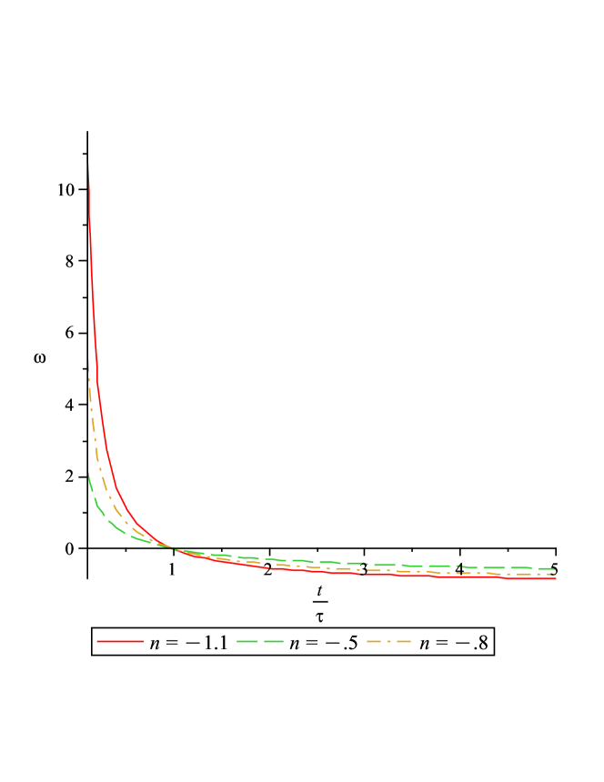
Figure 1: The plot of $\omega$ vs. t for different values of n in early epoch.

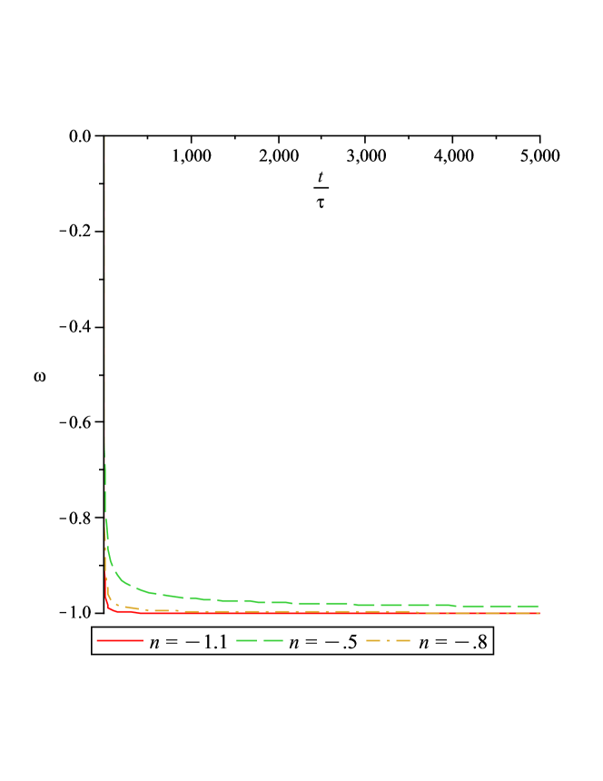
Figure 2: The plot of $\omega$ vs. t for different values of n in late time.

5.2 Calculation of the deceleration parameter

The deceleration parameter $q$ is a very important factor for understanding cosmic evolution. Particularly, after the emergence of the idea of an accelerating Universe, the role of this parameter has become even more important. This is because some recent works [40, 41, 42] have demonstrated that the present acceleration is a phenomenon of the recent past and was preceded by a decelerating phase. This cosmological picture supports the presently favored $\Lambda$-CDM Universe. So, during cosmic evolution the deceleration parameter $q$ must have undergone a change of sign from a positive to a negative value. So, calculation of $q$ from our model is essential for detecting a possible signature flip of $q$.

Now, using equations (9) and (35) we can obtain

$$q=-\left[1+\frac{\dot{H}}{H^{2}}\right]=-[1-1.5\Omega_{m}(t/\tau)^{n}].$$ (41)

Equation (42) shows that in the four dimensional case the expression for $q$ contains a time factor and hence with a suitable choice of $n$, $q$ can show its change of sign (Figs 3 and 4). Similarly, in the five dimensional case, using equations (26) and (38) the expression for $q$ reduces to

$$q=-[1-\Omega_{m}(t/\tau)^{n}].$$ (42)

Equation (42) shows that $q$ is time-dependent for the five dimensional case also and hence may change its sign during cosmic evolution (Figs 5 and 6). So, for $\Lambda\sim(\dot{a}/a)^{2}$ model, $q$ shows the possibility of a change of sign in both four and five dimensions. Since $\Lambda\sim(\dot{a}/a)^{2}$ and $\Lambda\sim\rho$ models are equivalent, it is clear that $\Lambda\sim\rho$ model will also show change of sign of $q$.

Again, $q$ can be written in terms of $\omega$ as

$$q=-[1-1.5\Omega_{m}(1+\omega)],$$ (43)

in the four dimensional case and

$$q=-[1-\Omega_{m}(1+\omega)],$$ (44)

in the five dimensional case.

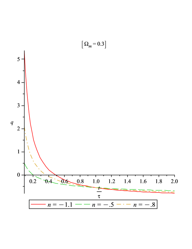
Figure 3: The plot of q vs. t for different values of n with fixed $\Omega_{m}$ in four dimension.

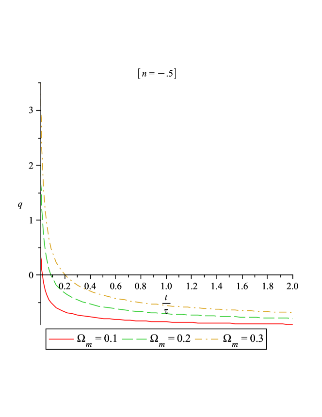
Figure 4: The plot of q vs. t for different values of $\Omega_{m}$ with fixed n in four dimension.

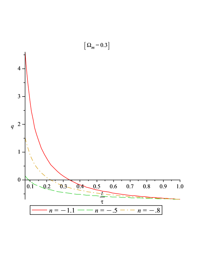
Figure 5: The plot of q vs. t for different values of n with fixed $\Omega_{m}$ in five dimension.

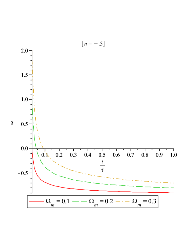
Figure 6: The plot of q vs. t for different values of $\Omega_{m}$ with fixed n in five dimension.

Now, considering various experimental and theoretical results, one can safely assume that the present value of the cosmic matter-energy density ($\Omega_{m0}$)as $0.33$ [25] (though seems rather a bit high value as given WMAP5 results). So, for the present dust-filled Universe ($\omega=0$), in the four dimensional case the value of $q$ comes out as $-0.505$ which is in nice agreement with the present accepted range of $q$ for an accelerating Universe [39]. For the five dimensional case, $q=-0.67$ for the same set of values of $\Omega_{m0}$ and $\Omega$ and hence that also supports the idea of an accelerating Universe.

6 Discussion

Although some specific constant values for the equation of state parameter $\omega$ are used for different phases of the cosmic evolution, that technique suffers from some kind of discreteness problem. The transition from one cosmic era to another can be understood better with a variable $\omega$. So, in order to have a continuous picture of cosmic evolution, $\omega$ should be regarded as time-dependent. In the previous sections, by selecting a simple power law expression of $t$ for the equation of state parameter $\omega$, equivalence of the models $\Lambda\sim(\dot{a}/a)^{2}$ and $\Lambda\sim\rho$ has been established in both four and five dimensions. In the four dimensional case, the parameters of the two equivalent models bear the same relationship with cosmic matter and vacuum energy densities as was found by Ray et al. [25] for constant $\omega$. But in five dimensions, the relationship of the same two parameters with $\Omega_{m}$ and $\Omega_{\Lambda}$ differ from that of Pradhan et al. [26]. It has also been possible to show that the sought-for signature flipping of the deceleration parameter $q$ can be obtained by suitable choice of $n$ in both four and five dimensions. This feature of the work satisfies an important criterion of $\Lambda$-CDM cosmology. It should be mentioned that the model $\Lambda\sim(\ddot{a}/a)$ which was shown to be equivalent to the present two $\Lambda$ models by Ray et al. [25] (in four dimensions) as well as by Pradhan et al. [26] (in five dimension) is found not to be equivalent to the two models considered here when $\omega$ is time-dependent.

If we now look at the plots, our observations regarding these are as follows :
(1) The plots (Figs 1 and 2) for $\omega$ show that in the early stage, it was positive i.e. in the early stages, the Universe was matter-dominated. The plots for $q$ also support this (i.e. decelerating phase of the Universe). At late times it is evolving with negative values (i.e. at the present time). The earlier real matter later on converted to the dark energy-dominated phase of the Universe. It, finally, ends up at $\omega=-1$, representing a cosmological constant dominated Universe;
(2) The plots (Figs 3 - 6) for $q$ show that in the early stages the Universe was in a decelerating phase and at late times, it is in an accelerating one.

Finally, the models under consideration are shown to be equivalent in both four and five dimensions and extension to the fifth dimension do not present us any basically new physical feature than the four dimensional case. So, a natural question can be raised: is there any justification for extension to five dimensions under the framework of general relativity? In this connection we would like to mention the works of Kapner et al. [43] and Rahaman et al. [44] where it is shown that extension of four dimensional general relativity to higher dimensions becomes mostly ineffective.

REFERENCES

- [1] J. Dunlop et al., Nature 381, 581 (1996).
- [2] H. Spinard et al., Astrophys. J. 484, 581 (1997)
- [3] A. G. Riess et al., Astron. J. 116, 1009 (1998).
- [4] S. J. Perlmutter et al., Astrophys. J. 517, 565 (1999).
- [5] J. Kujat et al., Astrophys. J. 572, 1 (2002).
- [6] M. Bartelmann et al., New Astron. Rev. 49, 199 (2005).
- [7] S. V. Chevron and V. M. Zhuravlev, Zh. Eksp. Teor. Fiz. 118, 259 (2000).
- [8] V. M. Zhuravlev, Zh. Eksp. Teor. Fiz. 120, 1042 (2001).
- [9] P. J. E. Peebles and B. Ratra, Rev. Mod. Phys. 75, 559 (2003).
- [10] R. Jimenez, New Astron. Rev. 47 761 (2003).
- [11] A. Das et al., Phy. Rev. D 72, 043528 (2005).
- [12] B. Ratra and P. J. E. Peebles, Phy. Rev. D 37, 3406 (1988).
- [13] M. S. Turner and M. White, Phy. Rev. D 56, R4439 (1997).
- [14] Caldwell et al., Phy. Rev. Lett. 80, 1582 (1998).
- [15] A. R. Liddle and R. J. Scherrer, Phy. Rev. D 59, 023509 (1999).
- [16] P. J. Steinhardt et al., Phy. Rev. D 59, 123504 (1999).
- [17] B. Bhui, B. C. Bhui and F. Rahaman, Astrophys. Space.Sc. 299, 61 (2005).
- [18] F. Rahaman, B. Bhui and B. C. Bhui, Astrophys. Space.Sc. 301, 47 (2006).
- [19] F. Rahaman, M. Kalam and S. Chakraborty, Acta Phys. Polon. B 40, 25 (2009).
- [20] K. Freese et al., Nucl. Phys. B 287, 797 (1987).
- [21] M. Özer and M. O. Taha, Nucl. Phys. B 287, 776 (1987).
- [22] W. Chen and Y. S. Yu, Phy. Rev. D 41, 695 (1990).
- [23] J. C. Carvalho et al., Phy. Rev. D 46, 2404 (1992).
- [24] J. A. Lima and J. M. F. Maia, Phy. Rev. D 49, 5597 (1994).
- [25] S. Ray, U. Mukhopadhyay and X. -H. Meng, Grav. Cosmol. 13, 142 (2007).
- [26] A. Pradhan et al., Int. J. Theor. Phys. 47 1751 (2008).
- [27] U. Mukhopadhyay, S. Ray and S. B. Duttachowdhury, Int. J. Mod. Phys. D. 17, 301 (2008).
- [28] U. Mukhopadhyay and S. Ray, N. B. U. Math. J. II, 51 (2009).
- [29] I. Dymnikova and M. Khlopov, Grav. Cosmol. Suppl. 4, 50 (1998).
- [30] I. Dymnikova and M. Khlopov, Mod. Phys. Lett. A 15, 2305 (2000).
- [31] I. Dymnikova and M. Khlopov, Eur. Phys. J. C 20, 139 (2001).
- [32] D. Huterer and M. S. Turner, Phys. Rev. D 64, 123527 (2001).
- [33] J. Weller and A. Albrecht, Phys. Rev. D 65, 103512 (2002).
- [34] D. Polarski and M.Chavellier, Int. J. Mod. Phys. D 10, 213 (2001).
- [35] E. V. Linder, Phy. Rev. Lett. 90, 91301 (2003).
- [36] U. Mukhopadhyay, P. P. Ghosh, M. Khlopov and S. Ray, gr-qc/07110686.
- [37] R. A. Knop et al., Astrophys. J. 598, 102 (2003)
- [38] M. Tegmark et al., Astrophys. J. 606, 702 (2004)
- [39] V. Sahni et al., Pramana 53, 937 (1999)
- [40] A. G. Riess, Astrophys. J. 560, 49 (2001).
- [41] L. Amendola, Mon. Not. R. Astron. Soc. 342, 221 (2003).
- [42] T. Padmanabhan and T. Roychowdhury, Mon. Not. R. Astron. Soc. 344, 823 (2003).
- [43] D. J. Kapner et al., Phys. Rev. Lett. 98, 021101 (2007).
- [44] F. Rahaman et al., Int J Theor Phys 48, 3124 (2009).