Observation of negative-frequency waves in a water tank: A classical analogue to the Hawking effect?

Abstract

The conversion of positive-frequency waves into negative-frequency waves at the event horizon is the mechanism at the heart of the Hawking radiation of black holes. In black-hole analogues, horizons are formed for waves propagating in a medium against the current when and where the flow exceeds the wave velocity. We report on the first direct observation of negative-frequency waves converted from positive-frequency waves in a moving medium. The measured degree of mode conversion is significantly higher than expected from theory.

PACS 04.70.Dy, 92.05.Bc

1 Introduction

The theory of Hawking radiation of black holes [1] connects three separate disciplines of physics — quantum mechanics, general relativity and thermodynamics [2] — and has been applied to test potential quantum theories of gravity [3, 4]. The radiation of astrophysical black holes is too feeble to be detectable, but laboratory analogues [5, 6, 7, 8] of the event horizon may demonstrate the physics behind Hawking radiation. Most candidates of artificial black holes rely on quantum fluids [8, 9, 10, 11, 12], but here we report on an experiment with a classical fluid: water [13]. A horizon is formed when flowing water exceeds the wave velocity. We observed a key ingredient of the classical mechanism behind Hawking radiation, the generation of waves with negative frequencies [1, 15, 16]. However, the measured conversion of positive into negative-frequency waves is significantly higher than expected from theory [13] for reasons we do not yet understand.

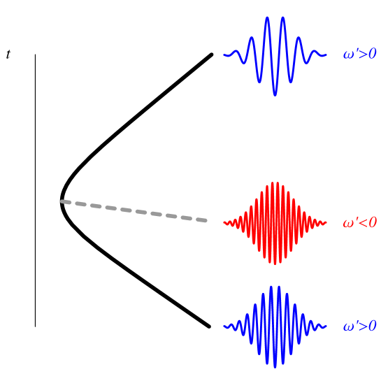
Figure 1: Tracing wave packets backwards in time at the horizon of a black hole. Schematic space-time diagram showing a wave packet escaping into space (top), potentially reaching an observer. This wave packet oscillates at positive frequencies, but it originates from two distinct waves, one with positive and another one with negative frequencies, shown below the escaping wave packet in the space-time diagram (for times in the past). This mixing of positive and negative frequencies is the classical root of the quantum Hawking radiation [1]. Note that the deflection of the incident waves at the horizon depends on the dispersion properties of the ”space-time medium” [17, 18, 19, 20, 21]. In astrophysics, these properties are unknown, in contrast to laboratory analogues.

In 1974 Hawking [1] predicted that black holes are not black: they radiate. The event horizon generates pairs of quanta; one particle of each pair emerges into space while its partner falls into the singularity. The quantum physics of pair creation at horizons is based on the features of classical wave-packet propagation [14, 15, 16] as follows: Figure 1 shows a wave packet escaping from the horizon. In a thought experiment, Hawking [14] traced such wave packets backwards in time and realized that they originate from two distinct waves: one oscillating with positive frequencies and another one with negative frequencies. Note that one can visualize negative frequencies in the way waves propagate in space and time, i.e in space-time diagrams or videos, but negative frequencies do not directly appear in snapshots of wave packets. Figure 2 compares the space-time diagrams of ordinary positive-frequency waves with the behavior of negative-frequency waves. The figure shows that the lines of equal phase in space-time have negative slopes for negative frequencies, as we discuss in Sec. 2.

Figure 2: Positive versus negative-frequency waves. The left diagram shows the space-time diagram of a wave with positive frequency, while the right diagram shows a negative-frequency wave. Section 2 explains the physics of negative-frequency waves in moving media. The pictures show space-time diagrams of waves in media moving with uniform speed. The left diagram displays a wave with positive wavenumber $k$, whereas the right diagrams shows a wave with negative $k$ and negative frequency $\omega^{\prime}$ in the co-moving frame.

The distinction between positive and negative frequencies is important for quantum fields [14, 15, 16]: the positive frequencies distinguish the annihilation and the negative frequencies the creation operators. A process that mixes positive and negative frequencies thus creates particles; the horizon spontaneously emits radiation. Figure 1 illustrates the wave packets of the particles that escape into space; the particles that fall into the black hole are shown in figure 3. They originate from mixtures of the two initial wave packets of Figure 1. Therefore the created quanta appear in entangled pairs, one escaping, the other one falling into the singularity.

Figure 3: Hawking partner. Schematic space-time diagram of a wave packet propagating against the ”space-time flow” on the other side of the horizon, drifting towards the singularity of the black hole. Like the wave illustrated in Fig. 1 this wave packet originates from waves with positive and negative frequencies. These waves are mixtures of the escaping waves of Fig. 1 traced backwards in time; hence the escaping quanta and the in-falling quanta form entangled partners.

Seen from outside, the black hole turns out [14, 15, 16] to emit black-body radiation with a temperature [1] that is proportional to the surface gravity at the horizon, or, equivalently, inversely proportional to the size of the black hole, the Schwarzschild radius. Since Hawking’s prediction, the radiation of horizons has been regarded as a confirmation for black-hole thermodynamics [2] and as a crucial test case for quantum theories of gravity such as superstring theory [3] and loop quantum gravity [4].

However, near the event horizon, fields are subject to frequency shifts beyond the Planck scale [17, 18, 19, 20, 21], as Fig. 1 schematically illustrates: the incident wave packets oscillate at significantly higher frequencies than the outgoing waves. The mechanism that could limit the frequency shifting at the horizon of the astrophysical black hole is unknown. Hawking radiation may thus depend on as yet unknown physics or may not exist at all. There is no observational evidence for Hawking radiation in astrophysics yet; and it seems unlikely that there ever will be for practical reasons — radiation with characteristic thermal wavelengths in the order of the Schwarzschild radius, a few km for solar-mass black holes, is obscured by the cm-waves of the Cosmic Microwave Background.

Astrophysical black holes are too large for noticeable Hawking radiation, but laboratory analogues [5, 6, 8, 7] of black holes offer valuable insights into the mechanism of radiating horizons. Most analogues are based on a simple idea [8, 9, 10]: black holes behave like moving fluids. Consider waves with phase velocity $c^{\prime}$ in a medium of flow speed $u$. If the magnitude of $u$ exceeds $c^{\prime}$ waves can no longer propagate upstream; they are trapped beyond a horizon. The horizon creates wave-quanta [5, 6, 7, 8], the analogue of Hawking radiation [1], with an effective temperature that depends on the flow gradient at the horizon, the analogue [5, 6, 7, 8] of the surface gravity. The radiation is only noticeable if the temperature of the fluid lies below the effective Hawking temperature. Superfluids [8] like Helium-3 or ultracold quantum gases [11, 12] may form radiating horizons for their elementary excitations and so would moving optical media for photons [7, 22].

On the other hand, at the heart of the Hawking effect lies a classical process that can be demonstrated with classical fluids such as water: the generation of waves with negative frequencies. For this, one should reproduce the characteristic behavior of wave packets at horizons traced backwards in time illustrated in Fig. 1. This is possible with a time-reversed black hole — a white-hole horizon — as shown in Fig. 4. The horizon of the white hole corresponds to the following analogy: imagine a fast river flowing out into the sea, getting slower. Waves cannot enter the river beyond the point where the flow speed exceeds the wave velocity; beyond this point the river resembles an object that nothing can enter, the white hole. Such wave blocking has been comprehensively studied in the fluid-mechanics literature [23, 24, 25, 26, 27, 28], but to our knowledge the generation of negative-frequency waves has never been observed before.

Figure 4: White-hole horizon. In order to demonstrate in a laboratory setting the tracing of wave packets backwards in time at a black-hole horizon, one has to time-reverse Fig. 1. The time-reversed black hole is the white hole. The arrow indicates the direction of the moving medium that establishes a horizon for counter-propagating waves.

2 Negative frequencies

What are negative-frequency waves? Consider linear one-dimensional wave propagation in a moving medium: a wave with phase $\varphi$ propagates in the $x$ direction against the flow $u$. The phase evolves in time $t$ as

$$\varphi=\int\left(k\,\mathrm{d}x-\omega\,\mathrm{d}t\right)$$ (1)

where $k$ denotes the wavenumber and $\omega$ the frequency in the laboratory frame. Imagine we construct at each point $x$ a frame that is co-moving with the fluid. In the locally co-moving frames $\mathrm{d}x=\mathrm{d}x^{\prime}+u\,\mathrm{d}t^{\prime}$ and $\mathrm{d}t=\mathrm{d}t^{\prime}$, and so the phase evolves in terms of the co-moving coordinates as the integral of $k\,\mathrm{d}x^{\prime}-\omega^{\prime}\,\mathrm{d}t^{\prime}$ with

$$\omega^{\prime}=\omega-uk\,.$$ (2)

Equation (2) simply describes the Doppler effect — waves are frequency-shifted due to the motion of the medium. In a locally co-moving frame, $\omega^{\prime}$ can only depend on the wavenumber $k$ and the properties of the medium, but not explicitly on the position: $\omega^{\prime}$ is a function $\omega^{\prime}(k)$ that is given by the dispersion relation. The phase velocity $c^{\prime}$ is defined as $\omega^{\prime}/k$, whereas the group velocity is

$$v_{g}=\frac{\partial\omega}{\partial k}=v_{g}^{\prime}+u\,,\quad v_{g}^{\prime}=\frac{\partial\omega^{\prime}}{\partial k}\,.$$ (3)

What can we say about the dispersion relation in general? In isotropic media, $\omega^{\prime 2}$ is an even function of $k$, because waves should be able to propagate in positive and negative directions in the same way. Without loss of generality we assume that the medium moves in the negative direction (from the right to the left). In this case, counter-propagating waves have positive phase velocities $c^{\prime}$. Therefore we take the branch of $\omega^{\prime}$ where $\omega^{\prime}/k$ is positive, i.e. where $c^{\prime}$ is an odd function of $k$ that is positive for positive $k$. We also assume that the counter-propagating waves move with positive group-velocities $v_{g}^{\prime}$ in the medium and that the group-velocity dispersion of the medium is normal, i.e. $v_{g}^{\prime}$ monotonically decreases for increasing $|k|$. Figure  5 shows our specific case that satisfies these general requirements.

Suppose that the laboratory frequency $\omega$ is fixed. The wavenumber $k$ is given by the Doppler formula (2) and the dispersion relation $\omega^{\prime}(k)$. In general, the solution of this equation is multi-valued: each frequency $\omega$ corresponds to several wavenumbers $k$, i.e. to several physically allowed waves. As visualized in Fig. 5, the physically allowed waves are determined by the points $k$ where the line $\omega-uk$ intersects the curve $\omega^{\prime}(k)$. One of these wavenumbers $k$ is always negative, as Fig. 5 illustrates. Since $\omega^{\prime}$ is an odd function of $k$, the co-moving frequency $\omega^{\prime}$ must be negative for negative $k$, although the frequency $\omega$ in the laboratory frame is always positive. We call waves with negative co-moving frequencies negative-frequency waves. Imagine we display the wave propagation in a space-time diagram, see Fig. 2. According to Eq. (1) the lines of constant phase $\varphi$ have positive slopes $\mathrm{d}t/\mathrm{d}x$ for positive $k$ and negative slopes for negative $k$. We regard this behavior as the characteristic feature of negative-frequency waves.

Figure 5: Doppler formula (2) versus dispersion relation (4) for $\omega^{\prime}$ plotted in arbitrary units. The wavenumber $k_{i}$ describes the incident wave, $k_{b}$ the blue-shifted and $k_{h}$ the Hawking wave with negative wavenumber $k$ and negative frequency $\omega^{\prime}$.

Figure 5 shows that for negative-frequency waves the slope of the curve $\omega^{\prime}(k)$ is smaller than the slope of the Doppler line, smaller than $-u$. As a consequence of Eq. (3) the group velocity $v_{g}$ in the laboratory frame must be negative. Therefore, negative-frequency waves cannot be launched directly, but they can be the result of a mode conversion from incident positive-frequency waves.

3 Water waves

Following a suggestion by Schützhold and Unruh [13], we studied water waves in the channel schematically shown in Fig. 6. A ramp in the channel creates a gradient in flow speed. The flowing water forms a white-hole horizon, an object that waves cannot enter, when the flow $|u|$ matches the group velocity $\partial\omega^{\prime}/\partial k$ of the waves. Water waves — gravity waves — obey the dispersion relation [29]

$$\omega^{\prime 2}=gk\tanh(kh)$$ (4)

where $g$ denotes the gravitational acceleration of the Earth at the water surface and $h$ is the height of the channel. In the limit of long wavelengths, i.e. small wavenumbers $k$, the dispersion relation (4) reduces to $\omega^{\prime 2}=gh\,k^{2}$; waves propagate with $c^{\prime}=\sqrt{gh}$. We see from the Doppler formula (2) that, in this limit, $\omega^{\prime}$ is connected to $\omega$ and $k$ by a quadratic form, which defines a space-time geometry [30]. A rigorous analysis [13] proves that the propagation of water waves is exactly equivalent to wave propagation in space-time geometries, as long as $|k|$ is much smaller than $1/h$. So, in our case, the channel height $h$ serves as a simple analogue of the Planck scale; waves with wavelengths shorter than $h$ do not experience the effective space-time geometry anymore. Close to the horizon, the incident waves are compressed until $k$ reaches the scale of $1/h$.

Figure 6: Schematic diagram of the experiment.

To characterize the waves, we use the graphical solution of the Doppler formula (2) combined with the dispersion relation (4) shown in Fig. 5. For a given positive frequency $\omega$, either one or three real solutions exist, one negative and possibly two positive $k$. Only in the case of a positive solution will the wave-maker launch waves, because the group velocity (3) of the negative-frequency wave is negative. The slope of $\omega^{\prime}$ at the smallest positive $k$ is higher than the slope of the Doppler line $\omega-uk$. For this wavenumber the group velocity is positive: this $k$ describes the incident wave. When the incident wave propagates against the rising current, the slope of the Doppler line rises until the two positive $k$ merge. At this point, the flow matches the group velocity of the wave. The incident wave is converted into a short-wavelength wave; it is blue-shifted below the effective Planck scale $h$. For the blue-shifted wave, $\partial\omega^{\prime}/\partial k$ lies below the flow speed $|u|$: the blue-shifted wave drifts back with negative group velocity (3), but $k$ is positive and so is the frequency $\omega^{\prime}$. Figure 5 shows that such wave blocking [23, 24, 25, 26, 27, 28] cannot occur below a critical flow speed. In order to estimate [26] the critical $u$ we replace $\tanh(kh)$ in the dispersion relation (4) by the asymptotic value of $1$. A real $k$ ceases to exist when the discriminant of the resulting quadratic equation vanishes, for $|u|=u^{*}=g/(4\omega)$. Since the dispersion curve (4) lies below the asymptotics, this procedure [26] gives an overestimation of the critical flow speed.

The horizon also converts [19, 20, 21] by tunnelling a part of the incident wave into the negative-$k$ branch of Fig. 5 that has a positive slope, generating a wave with negative co-moving frequency, the classical analogue of Hawking radiation. In fluid dynamics, the blue-shifted waves have been discussed and observed in connection with wave-blocking [23, 24, 25, 26, 27, 28] but to our knowledge the negative-frequency waves have neither been theoretically analyzed in the fluid-dynamics literature nor experimentally observed.

4 Experiment

We performed our experiment at ACRI, a private research company working on environmental fluid mechanics problems such as coastal engineering. The Génimar Laboratory, a department of ACRI, features a wave-tank $30\mathrm{m}$ long, $1.8\mathrm{m}$ wide and $1.8\mathrm{m}$ deep. The wave-maker is of piston-type and can generate waves with periods ranging from $0.6\mathrm{s}$ to $2.5\mathrm{s}$ with typical amplitudes around $5\mathrm{cm}$ to $30\mathrm{cm}$. A current can be superimposed in the same direction as the wave propagation or in the opposite one, with a maximum flow rate around $1.2\mathrm{m}^{3}/\mathrm{s}$. To generate a water-wave horizon, we insert a ramp immersed in water, with positive and negative slopes separated by a flat section; and send on it a train of waves against the reverse fluid flow produced by the pump. At the place where the flow speed equals the group velocity of the waves a horizon is created. The geometrical parameters are: maximum water height $1.4\mathrm{m}$ or $1.6\mathrm{m}$; positive slope $15.5^{\circ}$; length of the flat part $6\mathrm{m}$; minimum water height $30\mathrm{cm}$ or $50\mathrm{cm}$; negative slope $18.5^{\circ}$. We fix the physical characteristics of the waves, period and amplitude, and only vary the background flow. We record the waves with the three video cameras indicated in Fig. 6. As the background velocity is turbulent (the Reynolds number based on the water height is very large) and varies with depth, the horizon should be deduced from the mean velocity $\langle u(h,t)\rangle$ measured at the interface between air and water; the brackets denote time averaging. Due to experimental constraints, we measured the background flow with a MHD sensor averaged during $10\mathrm{s}$. The velocity profile on the flat part of the background flow is plug-like. Our first control parameter is $u_{\mathrm{max}}$, the maximum of the counter-current plug velocity over the flat part of the geometric profile without water waves. We have checked that the velocity profiles are similar along a cross section of the tank. The second control parameter is the period of oscillations of the wave-maker. Both parameters are displayed in the phase diagram of Fig. 7.

Figure 7: Phase diagram of our experiment. Each circle corresponds to a run with wave period $T=2\pi/\omega$ and maximal flow speed $u_{\mathrm{max}}$. The dots indicate runs where we observed negative-frequency waves, the squares runs with horizons. In regimes without horizons we saw a transition to mode conversion into purely positive frequencies below the lower dotted line in the diagram. The points (a) and (b) indicate the parameters used in Fig. 8.

In our experiments, we observed indications of wave conversion in the presence of horizons, but the cleanest data we obtained was for flow speeds just below the horizon condition. In this case, the wave conversion still occurs [31], although it is reduced in magnitude. Without a group-velocity horizon, the flow is much quieter, wave breaking and turbulence are significantly reduced. Figure 8 shows the space-time diagrams of two typical cases, one illustrating the conversion into short waves with positive phase velocity, and the other showing waves with negative frequency superposed on the incident waves.

Figure 8: Space-time diagrams, showing water waves propagating from the left to the right with the parameters (a) and (b) of Fig. 7, initial amplitude $5\mathrm{cm}$ and water height $1.4\mathrm{m}$. No horizon is formed, but mode conversion still occurs. (a) conversion into the positive-frequency waves $k_{b}$ of Fig. 5; (b) waves with negative frequency (negative phase slope as shown in Fig. 2). The images were extracted from the video data recorded with camera 1 of Fig. 6. The right pictures display time traces along the lines indicated in the space-time diagrams. The traces show that the additional waves are periodic in $T$, indicating that they are converted incident waves.

5 Numerical simulations

In order to test whether conversion into negative-frequency modes occurs even in the absence of a horizon, we applied Unruh’s method [19] for numerically simulating waves in moving media. We consider wave packets propagating against the current in a simple one-dimensional model for the flow, using periodic boundary conditions, and analyse the mode conversion. This simulation does not describe the influence of turbulence, nonlinearity, the three-dimensional aspects of our experiment nor the variation of the flow with water depth, but it captures the qualitative aspects of the Hawking effect and proves that the mode conversion can occur without a horizon, a regime where the experiment is least affected by wave breaking and turbulence. A related example of Hawking radiation without horizon has been studied before [31] that qualitatively agrees with our findings, although our case is significantly more extreme. Figure 9 shows the result of a wave packet interacting with the spatially dependent flow given by

$$u(x)=-u_{0}-u_{1}[\tanh(ax)-\tanh(a(x-x_{0}))]\,;$$ (5)

the fluid moves left at velocity $-u_{0}$ at $x<0$, decreasing to $-u_{0}-u_{1}$ between $x=0$ and $x=x_{0}$ and returning to $-u_{0}$ at $x>x_{0}$. Gravity waves with the perturbation $w(t,x)$ of the velocity potential obey the equation [13]

$$(\partial_{t}+\partial_{x}u)(\partial_{t}+u\partial_{x})w=\mathrm{i}g\partial_{x}\tanh(-\mathrm{i}h\partial_{x})w\,,$$ (6)

giving the dispersion relation (4). The wave packet propagates to the right; the flow speed nowhere reaches a value great enough to block the packet and create a white-hole horizon. When the packet travels into the faster-flow region $x>0$ some of it tunnels into the blue-shifted root of the dispersion relation and this part propagates back to the left. There is also some tunnelling into the negative $k$ root; this portion has shorter wavelength than the blue-shifted waves and travels more quickly to the left. The simulation shows that negative-frequency waves can be generated without the presence of a horizon. The slope in the simulation is not realistic for our experiment, however, otherwise there would be no visible $k_{h}$ in the simulation. But in the experiment negative-frequency waves were clearly observed. Apparently, the simple model [13] we used does not capture all the complexity of our system.

Figure 9: Wave-packet simulations. The left figure shows the incident wave packet traveling in positive $x$ direction, the right figure its partial conversion into two wavelength components travelling in negative $x$ direction. The components separate because of their different group velocities; the Hawking component is visible in the centre of the figure. The wrap-around is caused by periodic boundary conditions and most of the packet that travels to the right beyond the conversion region is not shown. We used the parameters $u_{0}=0.7\mathrm{m}/\mathrm{s}$, $u_{1}=0.122\mathrm{m}/\mathrm{s}$, $a=12\mathrm{m}^{-1}$, $h=0.6\mathrm{m}$, $T=2.5\mathrm{s}$.

6 Conclusions

We believe we have made the first direct observation of the conversion of incident waves with positive frequency into negative-frequency waves in a moving medium. In astrophysics, such a mode conversion occurs at the event horizon of black holes. It represents the classical mechanism at the heart of Hawking radiation [1]. However, we were surprised how strong the experimentally observed mode conversion is, because in numerical simulations of a simple model [13] we saw a significantly lower conversion. This model takes into account the correct dispersion relation (4), but it does not describe turbulence, nonlinearity, nor the three-dimensional nature of our experiment. It would be highly desirable to find out exactly what happens to water waves at horizons. Unfortunately, with the current set-up we have not sufficient data to characterize the actual process of mode conversion in detail. It is conceivable that we have seen a new fluid-mechanics phenomenon that significantly enhances the Hawking effect. Could it be a nonlinear mode conversion, a nonlinear process generating harmonics with negative frequencies? We observed that the incident waves become steeper as they propagate against the current. Hence, locally, waves can be generated close to the crest, possibly with additional vorticity creation, where geometric cusps could develop through nonlinear effects. These crests waves are then swept away by the flow. Moreover, it remains to be checked in future experiments whether a transverse curvature of the wave crest could also be responsible for the creation of negative-frequency waves. In any case, despite the limitations of our present experiment, we have found clear evidence for negative-frequency waves. In this way, we have demonstrated a key ingredient of the quantum radiation of black holes using a relatively simple classical laboratory analogue, waves in a water tank.

References

- [1] S. M. Hawking, Nature 248, 30 (1974).
- [2] J. D. Bekenstein, Phys. Rev. D 7, 2333 (1973).
- [3] M. B. Green, J. H. Schwarz, and E. Witten, Superstring Theory (Cambridge University Press, Cambridge, 1987).
- [4] C. Rovelli, Living Rev. Rel. 1, 1 (1998).
- [5] M. Novello, M. Visser, and G. E. Volovik (editors), Artificial black holes (World Scientific, Singapore, 2002).
- [6] W. G. Unruh and R. Schützhold, Quantum Analogues: From Phase Transitions to Black Holes and Cosmology (Springer, Berlin, 2007).
- [7] T. G. Philbin, C. Kuklewicz, S. Robertson, S. Hill, F. König, and U. Leonhardt, Science (in press); arXiv:0711.4796; arXiv:0711.4797.
- [8] G. E. Volovik, The Universe in a Helium Droplet (Clarendon Press, Oxford, 2003).
- [9] W. G. Unruh, Phys. Rev. Lett. 46, 1351 (1981).
- [10] M. Visser, Class. Quantum Grav. 15, 1767 (1998).
- [11] L. J. Garay, J. R. Anglin, J. I. Cirac, and P. Zoller, Phys. Rev. Lett. 85, 4643 (2000).
- [12] S. Giovanazzi, Phys. Rev. Lett. 94, 061302 (2005).
- [13] R. Schützhold and W. G. Unruh, Phys. Rev. D 66, 044019 (2002).
- [14] S. M. Hawking, Commun. Math. Phys. 43, 199 (1975).
- [15] R. Brout, S. Massar, R. Parentani, and Ph. Spindel, Phys. Rep. 260, 329 (1995).
- [16] N. D. Birrell and P. C. W. Davies, Quantum Fields in Curved Space (Cambridge University Press, Cambridge, 1982).
- [17] G. t’Hooft, Nucl. Phys. B 256, 727 (1985).
- [18] T. Jacobson, Phys. Rev. D 44, 1731 (1991).
- [19] W. G. Unruh, Phys. Rev. D 51, 2827 (1995).
- [20] R. Brout, S. Massar, R. Parentani, and Ph. Spindel, Phys. Rev. D 52, 4559 (1995).
- [21] S. Corley and T. Jacobson, Phys. Rev. D 54, 1568 (1996).
- [22] U. Leonhardt, Rep. Prog. Phys. 66, 1207 (2003).
- [23] M. W. Dingemans, Water Wave Propagation over Uneven Bottoms - Part 1: Linear Wave Propagation (World Scientific, Singapore, 1997).
- [24] D. H. Peregrine, Adv. Appl. Mech. 16, 9 (1976).
- [25] I. G. Jonsson, Wave-current interactions in B. Le Méhauté and B. Hanes (editors) The sea (John Wiley and Sons, New York, 1990).
- [26] A. Chawla and J. T. Kirby, J. Geophys. Res. - Oceans 107, 3067 (2002).
- [27] I. K. Suastika, M. P. C. de Jong, and J. A. Battjes, Experimental study of wave blocking, in Proc. 27th Int. Conf. Coastal Eng., Sydney, 2000, Vol.1, pp. 227.
- [28] I. K. Suastika, Wave Blocking, PhD Thesis, Technische Universiteit Delft, The Netherlands, 2004, see http://repository.tudelft.nl/file/275166/201607.
- [29] L. D. Landau and E. M. Lifshitz, Fluid mechanics (Elsevier, Amsterdam, 2004).
- [30] L. D. Landau and E. M. Lifshitz, The classical theory of fields (Butterworth-Heinemann, Oxford, 1995).
- [31] C. Barceló, S. Liberati, S. Sonego, and M. Visser, Phys. Rev. Lett. 97, 171301 (2006).