Approximate $w_{\phi}\sim\Omega_{\phi}$ Relations in Quintessence Models

Abstract

Quintessence field is a widely-studied candidate of dark energy. There is “tracker solution” in quintessence models, in which evolution of the field $\phi$ at present times is not sensitive to its initial conditions. When the energy density of dark energy is neglectable ($\Omega_{\phi}\ll 1$), evolution of the tracker solution can be well analysed from “tracker equation”. In this paper, we try to study evolution of the quintessence field from “full tracker equation”, which is valid for all spans of $\Omega_{\phi}$. We get stable fixed points of $w_{\phi}$ and $\Omega_{\phi}$ (noted as $\widehat{w}_{\phi}$ and $\widehat{\Omega}_{\phi}$) from the “full tracker equation”, i.e., $w_{\phi}$ and $\Omega_{\phi}$ will always approach $\widehat{w}_{\phi}$ and $\widehat{\Omega}_{\phi}$ respectively. Since $\widehat{w}_{\phi}$ and $\widehat{\Omega}_{\phi}$ are analytic functions of $\phi$, analytic relation of $\widehat{w}_{\phi}\sim\widehat{\Omega}_{\phi}$ can be obtained, which is a good approximation for the $w_{\phi}\sim\Omega_{\phi}$ relation and can be obtained for the most type of quintessence potentials. By using this approximation, we find that inequalities $\widehat{w}_{\phi}<w_{\phi}$ and $\widehat{\Omega}_{\phi}<\Omega_{\phi}$ are statisfied if the $w_{\phi}$ (or $\widehat{w}_{\phi}$) is decreasing with time. In this way, the potential $U(\phi)$ can be constrained directly from observations, by no need of solving the equations of motion numerically.

I Introduction

Present astronomical observations require the existence of dark energy, a significant component of the universe with a negative pressure Riess:1998cb ; Riess:2004nr ; Riess:2006fw ; Spergel:2003cb ; Komatsu:2008hk . Though it has been more than ten years since its discovery, one is yet to tell what the dark energy is. We are still analyzing properties of dark energy from observational data and seeking suitable candidates. Most properties of dark energy depend on two parameters: the equation of state $w_{de}$ and the fractional energy density $\Omega_{de}$. Once the $w_{de}\sim\Omega_{de}$ relation is obtained, we know almost all we need. At present, it is still not possible to constrain the evolution of dark energy from observations Daly:2004gf ; Mignone:2007tj ; Sullivan:2007pd . There are only definite constraints of present values of $w_{de}$ and $\Omega_{de}$ from observations: $w_{de}^{(0)}$ is rather close to $-1$ and $\Omega_{de}^{(0)}$ is dominating (about 70%) Lazkoz:2007zk ; Copeland:2006wr ; Mantz:2007qh . More constraints on $w_{de}$ and $\Omega_{de}$ will be forthcoming from future observations, to get the evolution of the $w_{de}\sim\Omega_{de}$ relation from the observations, more theoretical efforts should be made.

At present, the most economical candidate of dark energy is still the cosmological constant $\Lambda$, whose equation of state $w_{\Lambda}=-1$. There is only a free parameter $\Omega_{\Lambda}$ in the flat $\Lambda$CDM model. But it suffers from several problems, such as the coincidence problem and the fine tuning problem. Another well studied candidate is the quintessence $\phi$, a slowly rolling scalar field, analogous to the inflaton. Its equation of state is $w_{\phi}=(\dot{\phi}^{2}/2-U)/(\dot{\phi}^{2}/2+U)$ so one has $-1\leq w_{\phi}\leq 1$. In quintessence models, the coincidence problem and the fine tuning problem can be alleviated Copeland:2006wr . For example, there are tracker solutions for certain type of quintessence models, in which the evolution of $\phi$ today is not sensitive to its initial conditions at early times Steinhardt:1999nw . The coincidence problem thus becomes less severe. But it is difficult to find quintessence models with analytic solutions of equation-of-motion, due to the existence of background matters (dark matter, baryon and radiations). To study evolutions of quintessence models and to be compared with observations, one usually has to solve the equations numerically. There are efforts to find analytic approximations for solutions of equations of motions, such as Watson:2003kk which gives a first order approximation solution for inverse power law potentials.

In this paper, we will try to approximate the $w_{\phi}\sim\Omega_{\phi}$ relation at the recent $\Omega_{\phi}$ dominating period in a semi-analytic way. To make sure that the evolution of $\phi$ at present only depends on $U(\phi)$, we assume there was tracking solution at early times. In Steinhardt:1999nw , conditions for the existence of tracker solution was given by the “tracker equation”, which is a differential equation for $w_{\phi}$. But this “tracker equation” are only valid as $\Omega_{\phi}\ll 1$. For our purpose, we need a full tracker equation that is valid for all $\Omega_{\phi}$ without conditions attached. Such an equation has been obtained Scherrer:2005je ; Chiba:2005tj ; Lee:2006gx and will be used here to study evolutions of quintessence models.

The paper is organized as follows. In section II, we introduce two new functions $\widehat{w}_{\phi}$ and $\widehat{\Omega}_{\phi}$ which are fixed points of the full tracker equation. Assuming that $\Gamma\equiv U^{\prime\prime}U/U^{\prime 2}$ and $\epsilon\equiv(U^{\prime}/U)^{2}/2$ are nearly constant, we find that the fixed points are stable for $w_{\phi}$ and $\Omega_{\phi}$ if $\Gamma\geq 1$. If $\Gamma$ and $\epsilon$ do not evolve extremely fast, the relation of $w_{\phi}\sim\Omega_{\phi}$ will always approach to that of $\widehat{w}_{\phi}\sim\widehat{\Omega}_{\phi}$. In section III we show comparisons between {$\widehat{w}_{\phi}(\phi)$, $\widehat{\Omega}_{\phi}(\phi)$} and {$w_{\phi}(\phi)$, $\Omega_{\phi}(\phi)$} numerically for several typical quintessence models. The relation of $\widehat{w}_{\phi}\sim\widehat{\Omega}_{\phi}$ is shown to be a good approximation for the $w_{\phi}\sim\Omega_{\phi}$ relation. In section IV we show how to constrain $U(\phi)$ directly from observational conditions on $w_{\phi}$ and $\Omega_{\phi}$ through $\widehat{w}_{\phi}$ and $\widehat{\Omega}_{\phi}$. Observational conditions are converted to simple inequalities for $U(\phi)$. We conclude in section V with discussions.

II Get the approximation of $w_{\phi}\sim\Omega_{\phi}$ relations

The equations of motion for quintessence field are

$$\ddot{\phi}+3H\dot{\phi}+U^{\prime}=0$$

$$H^{2}\equiv(\frac{\dot{a}}{a})^{2}=\frac{1}{3}(\rho_{m}+\rho_{r}+\frac{1}{2}\dot{\phi}^{2}+U)$$ (1)

from which one gets the equations for $w_{\phi}$ and $\Omega_{\phi}$:

$$\epsilon = \frac{3(1+\omega_{\phi})}{2\Omega_{\phi}}(1+\frac{\dot{x}}{6})^{2}$$ (2)

$$\Gamma-1 = \frac{\omega_{b}-\omega_{\phi}}{2(1+\omega_{\phi})}-\frac{2}{(1+\omega_{\phi})}\frac{\ddot{x}}{(6+\dot{x})^{2}}-\frac{1+\omega_{b}-2\omega_{\phi}}{2(1+\omega_{\phi})}\frac{\dot{x}}{6+\dot{x}}$$ (3)

$$-\frac{3(\omega_{b}-\omega_{\phi})}{(1+\omega_{\phi})(6+\dot{x})}\Omega_{\phi}$$

where

$$x\equiv\frac{1+\omega_{\phi}}{1-\omega_{\phi}}=\frac{1}{2}{\dot{\phi}^{2}\over U},~{}~{}~{}\dot{x}\equiv{d\ln{x}\over d\ln{a}},~{}~{}~{}\ddot{x}\equiv{d^{2}\ln{x}\over d\ln{a}^{2}}$$

and $a$ is the expansion factor. We have assumed a flat universe ($\Omega_{b}+\Omega_{\phi}=1$) and set $M_{pl}\equiv 1/\sqrt{8\pi G}=1$. The subscript $b$ represents the dominating background matter. As $\Omega_{\phi}\ll 1$ at early times, Eq.(3) reduces to the “tracker equation” in Steinhardt:1999nw . At the recent acceleration era, $\Omega_{\phi}$ is dominating and can not be neglected. One must use the full tracker equation Eq.(3). Note also $w_{b}=0$ in this case. In this paper, we assume that there was a long enough tracking period at early times, so that the evolution of the field at present depends only on $U(\phi)$.

Eliminating $\Omega_{\phi}$ in Eq.(3) by using Eq.(2), one gets:

$$\Gamma-1 = -\frac{\omega_{\phi}}{2(1+\omega_{\phi})}-\frac{2}{(1+\omega_{\phi})}\frac{\ddot{x}}{(6+\dot{x})^{2}}$$ (4)

$$-\frac{1-2\omega_{\phi}}{2(1+\omega_{\phi})}\frac{\dot{x}}{6+\dot{x}}+\frac{\omega_{\phi}}{8\epsilon}(6+\dot{x})$$

For constant $\epsilon$ and $\Gamma$, the fixed point (also called critical point) of Eq.(4) (obtained by setting $\dot{x}=0$ and $\ddot{x}=0$):

$$\widehat{\omega}_{\phi}=\frac{1}{6}\left(-3-2\epsilon+4\epsilon\Gamma-\sqrt{(3-2\epsilon+4\epsilon\Gamma)^{2}-24\epsilon}\right)$$ (5)

is stable only if

$$\Gamma\geq\frac{5+3\widehat{\Omega}_{\phi}}{6+2\widehat{\Omega}_{\phi}}$$ (6)

where the $\widehat{\Omega}_{\phi}$ value of the fix point is obtained from Eq.(5) and (2) (also setting $\dot{x}=0$):

$$\widehat{\Omega}_{\phi}=\frac{1}{4\epsilon}\left(3-2\epsilon+4\epsilon\Gamma-\sqrt{(3-2\epsilon+4\epsilon\Gamma)^{2}-24\epsilon}\right)$$ (7)

When Eq.(6) is satisfied, $\widehat{\Omega}_{\phi}$ is also stable. In this case, ${\omega}_{\phi}$ and $\Omega_{\phi}$ will always approach $\widehat{\omega}_{\phi}$ and $\widehat{\Omega}_{\phi}$ respectively. In this paper, we will only study the case of $\Gamma\geq 1~{}~{}(i.e.,~{}w_{\phi}\leq w_{b})$, so Eq.(6) is guaranteed for all spans of $\widehat{\Omega}_{\phi}$.

$\Gamma$ and $\epsilon$ generally are not constants, as they are functions of $U(\phi)$. The above results are still valid if the evolution of $\widehat{w}_{\phi}$ is not extremely fast, which can be satisfied in the most quintessence models. In this case, $w_{\phi}$ and ${\Omega}_{\phi}$ will keep on chasing the dynamic $\widehat{w}_{\phi}$ and $\widehat{\Omega}_{\phi}$.

Giving the form of $U(\phi)$ of a quintessence model, one gets parametric functions $\widehat{w}_{\phi}(\phi)$ and $\widehat{\Omega}_{\phi}(\phi)$ from Eq.(5) and (7), and thus the analytic relation of $\widehat{w}_{\phi}\sim\widehat{\Omega}_{\phi}$. For certain models, there are simple and explicit relations of $\widehat{w}_{\phi}\sim\widehat{\Omega}_{\phi}$. For example, for power law potentials $U=U_{0}/\phi^{n}~{}~{}(n>0)$ one has:

$$\widehat{w}_{\phi}=-\frac{1}{1+n(1-\widehat{\Omega}_{\phi})/2}$$ (8)

The $\widehat{w}_{\phi}\sim\widehat{\Omega}_{\phi}$ relation is a good approximation for that of $w_{\phi}\sim{\Omega}_{\phi}$, as the evolution of $w_{\phi}\sim{\Omega}_{\phi}$ will approach that of $\widehat{w}_{\phi}\sim\widehat{\Omega}_{\phi}$. We will show this in the next section. In this way, evolutions of quintessence models can be studied directly from $U(\phi)$.

III Compared with numerical results

In this section we will show that ${\widehat{w}}_{\phi}$ and ${\widehat{\Omega}}_{\phi}$ are good approximations for $w_{\phi}$ and $\Omega_{\phi}$, and so is the $\widehat{w}_{\phi}\sim\widehat{\Omega}_{\phi}$ relation for that of $w_{\phi}\sim{\Omega}_{\phi}$. We have checked it for a variety type of quintessence potentials, and typical examples are shown in Fig. 1 and Fig. 2. The accuracy of this approximation is precise enough to study the evolution properties of quintessence models, especially the models that are favored by present observations. As $w_{\phi}$ must decrease from its tracking value (close to $w_{b}$) to present value (close to $-1$), we will only study models in which $w_{\phi}$ decreases monotonously ($\dot{x}<0$).

Figure 1: Evolution of $(1+\dot{x}/6)^{2}$ (solid lines), $(1+\widehat{w}_{\phi})/(1+w_{\phi})$ (dashed lines) and $\widehat{\Omega}_{\phi}/\Omega_{\phi}$ (dotted lines) with respect to $\Omega_{\phi}$. The potentials: I. $U=U_{0}e^{1/\phi}$; II. $U=U_{0}/\phi^{2}$; III. $U=U_{0}/\phi^{0.5}$. The last figure shows the deviation $\Delta$ of ${\widehat{w}}_{\phi}$ from $w_{\phi}$ for these models.

At first we estimate differences between $\widehat{w}_{\phi}$ and $w_{\phi}$ and between $\widehat{\Omega}_{\phi}$ and ${\Omega}_{\phi}$. The Eq.(2) can be rewritten as:

$$\frac{1+\widehat{w}_{\phi}}{\widehat{\Omega}_{\phi}}=\frac{1+\omega_{\phi}}{\Omega_{\phi}}(1+\frac{\dot{x}}{6})^{2}$$

$$\Rightarrow~{}~{}~{}~{}~{}(\frac{1+\widehat{w}_{\phi}}{1+w_{\phi}})\cdot(\frac{\widehat{\Omega}_{\phi}}{\Omega_{\phi}})^{-1}=(1+\frac{\dot{x}}{6})^{2}$$ (9)

For a variety of quintessence models, we have seen numerically that $(1+\widehat{w}_{\phi})/(1+w_{\phi})$ and $\widehat{\Omega}_{\phi}/\Omega_{\phi}$ have the similar evolving forms as that of $(1+\dot{x}/6)^{2}$ and $1>\widehat{\Omega}_{\phi}/\Omega_{\phi}\gtrsim(1+\dot{x}/6)^{2}>(1+\widehat{w}_{\phi})/(1+w_{\phi})$. Typical examples are shown in Fig. 1. If the evolution of $\widehat{w}_{\phi}$ (and $w_{\phi}$) is slower, the value of $\dot{x}$ will be closer to $0$, and the differences between $w_{\phi},~{}\Omega_{\phi}$ and their fixed points will be smaller.

Figure 2: The $w_{\phi}\sim\Omega_{\phi}$ relation (solid lines), the $\widehat{w}_{\phi}\sim\widehat{\Omega}_{\phi}$ relation (dashed lines) and the $\widetilde{w}_{\phi}\sim\widetilde{\Omega}_{\phi}$ relation (dotted lines) in the $w-\Omega$ space. The potentials: I. $U=U_{0}e^{1/\phi}$; II. $U=U_{0}/\phi^{2}$; III. $U=U_{0}/\phi^{0.5}$. The last figure shows the differences between the relation of $w_{\phi}\sim\Omega_{\phi}$ and that of $\widehat{w}_{\phi}\sim\widehat{\Omega}_{\phi}$ for these models ( $\delta=-[w(\Omega)-\widehat{w}(\widehat{\Omega}=\Omega)]/w(\Omega)$ ).

There is a lower bound $\dot{x}>6w_{\phi}/(1-2w_{\phi})$ given in Scherrer:2005je ; Chiba:2005tj . As $\widehat{\Omega}_{\phi}/\Omega_{\phi}$ is much closer to $1$ compared with $(1+\widehat{w}_{\phi})/(1+w_{\phi})$, one gets a upper bound for the deviation $\Delta$ of ${\widehat{w}}_{\phi}$ from $w_{\phi}$ by setting $\widehat{\Omega}_{\phi}/\Omega_{\phi}\simeq 1$ in Eq.(9):

$$\Delta\equiv\frac{\widehat{w}_{\phi}-w_{\phi}}{w_{\phi}}\lesssim\Delta_{m}=\frac{(2-3w_{\phi})(1+w_{\phi})}{(1-2w_{\phi})^{2}}$$ (10)

which is rather small when $w_{\phi}$ is close to $-1$, as shown in Fig. 1. Present observations indicate that $w_{\phi}$ is rather close to $-1$ at low redshift. For most models $\Delta$ is much smaller than this bound as $w_{\phi}$ is not so close to $-1$, as shown in Fig. 1. The deviation of $\widehat{\Omega}_{\phi}$ from $\Omega_{\phi}$ is also small.

The $\widehat{w}_{\phi}\sim\widehat{\Omega}_{\phi}$ relation thus is a good approximation for the $w_{\phi}\sim{\Omega}_{\phi}$ relation. Several examples are shown in Fig. 2. At the early tracking era, $\widehat{\Omega}_{\phi}<<1$ and the relation of $w_{\phi}\sim\Omega_{\phi}$ is almost the same as that of $\widehat{w}_{\phi}\sim\widehat{\Omega}_{\phi}$. When $\widehat{\Omega}_{\phi}$ becomes unnegligible, the curve of $\widehat{w}_{\phi}\sim\widehat{\Omega}_{\phi}$ will begin to get away from that of $w_{\phi}\sim\Omega_{\phi}$ in the $w-\Omega$ space. The curve of $w_{\phi}\sim\Omega_{\phi}$ will chase after that of $\widehat{w}_{\phi}\sim\widehat{\Omega}_{\phi}$. Normally $\widehat{w}_{\phi}$ will tend to $-1$ and $\widehat{\Omega}_{\phi}$ will tend to $1$ at last, and the two curves will be close to each other once again.

Empirically, we have also found a better approximation for the relation of $w_{\phi}\sim\Omega_{\phi}$ on the basis of $\widehat{w}_{\phi}$ and $\widehat{\Omega}_{\phi}$:

$$\widetilde{w}_{\phi}=\widehat{w}_{\phi}+\frac{(2+\widehat{w}_{\phi})\widehat{\Omega}_{\phi}-2\widehat{w}_{\phi}-1}{5-3\widehat{\Omega}_{\phi}}(1+\widehat{w}_{\phi}),~{}~{}~{}~{}\widetilde{\Omega}_{\phi}=\widehat{\Omega}_{\phi}$$ (11)

The curve of $\widetilde{w}_{\phi}\sim\widetilde{\Omega}_{\phi}$ is much closer to that of $w_{\phi}\sim\Omega_{\phi}$, as shown in Fig. 2.

IV Constrain quintessence potentials

In the above, we have obtained approximations $\widehat{w}_{\phi}$ and $\widehat{\Omega}_{\phi}$ for $w_{\phi}$ and $\Omega_{\phi}$ which are analytic functions of $U(\phi)$. We will show how to constrain $U(\phi)$ directly from observational results on $w_{de}$ and $\Omega_{de}$ through $\widehat{w}_{\phi}$ and $\widehat{\Omega}_{\phi}$. Present data seems to indicate that $w_{de}^{(0)}<-0.8$ and $0.7\lesssim\Omega_{de}^{(0)}<0.8$ Lazkoz:2007zk ; Mantz:2007qh . As more conditions on dark energy to be obtained in future observations, more quintessence models can be checked with directly by using our method.

At the early tracking era $w_{\phi}$ was close to $w_{r}=1/3$ Bludman:2004az ; Zlatev:1998tr , and present $w_{de}^{(0)}$ is very close to $-1$. Taking this for guidance, here we consider only quintessence models in which $w_{\phi}~{}$(and $\widehat{w}_{\phi}$) keeps on decreasing monotonously ($\dot{x}<0$). This is guaranteed if $U(\phi)$ satisfies the equation:

$$\frac{d\ln{(\Gamma-1)}}{d\ln{U}}<\frac{3}{2\epsilon}(1-\frac{1}{2\Gamma-1})$$ (12)

In this case, one finds the following inequalities

$$\widehat{w}_{\phi}<w_{\phi},~{}~{}~{}~{}\widehat{\Omega}_{\phi}<\Omega_{\phi}$$ (13)

if the evolution of $w_{\phi}$ is not extremely fast. Intuitively, the curve of $\widehat{w}_{\phi}\sim\widehat{\Omega}_{\phi}$ is always on the up side of that of $w_{\phi}\sim\Omega_{\phi}$ in the $w-\Omega$ space, as shown in Fig. 2.

With the help of inequalities (13), $U(\phi)$ can be constrained directly from conditions on $(w_{de},\Omega_{de})$. Take

$$(w_{de}^{(0)}<-0.8,\Omega_{de}^{(0)}<0.8)$$ (14)

for illustration Caldwell:2005tm . Since $\widehat{w}_{\phi}$ decreases monotonously as $\widehat{\Omega}_{\phi}$ increases, we thus have $\widehat{w}_{\phi}(\widehat{\Omega}_{\phi}=0.8)<-0.8$. This inequality can be converted to:

$$\Gamma(\epsilon=3/8)>7/5$$ (15)

which is a necessary condition for inequalities (14).

Table 1: Constraints of typical potentials of quintessence

$U(\phi)~{}(n>0,\phi>0)$	$\epsilon\equiv\frac{1}{2}(\frac{U^{\prime}}{U})^{2}$	$\Gamma\equiv\frac{U^{\prime\prime}U}{U^{\prime 2}}$	$\Gamma(\epsilon=\frac{3}{8})>\frac{7}{5}$	$\Gamma(\epsilon=\frac{3}{28})<\frac{77}{20}$
$\frac{U_{0}}{\phi^{n}}$	$\frac{n^{2}}{2\phi^{2}}$	$1+\frac{1}{n}$	$n<\frac{5}{2}$	$n>\frac{20}{57}$
$U_{0}e^{n/\phi}$	$\frac{n^{2}}{2\phi^{4}}$	$1+\frac{2\phi}{n}$	$n<\frac{50}{\sqrt{3}}$	$n>1$
$\frac{U_{0}}{\phi^{n}}e^{\phi^{2}/2}$	$\frac{(n-\phi^{2})^{2}}{2\phi^{2}}$	$1+\frac{(n+\phi^{2})}{(n-\phi^{2})^{2}}$	$n>0$	$\emptyset$

If $w_{\phi}$ is too close to $-1$, it will be difficult to distinguish quintessence models from the cosmological constant Caldwell:2005tm . Take $w_{\phi}>-0.95$ for illustration. It is then easy to see that $\widehat{w}_{\phi}(\widehat{\Omega}_{\phi}=0.7)>-0.95$ is a sufficient condition for ($w_{\phi}^{(0)}>-0.95$, $\Omega_{de}^{(0)}>0.7$). Equivalently,

$$\Gamma(\epsilon=3/28)<77/20$$ (16)

Listed in Table I are the constraints on parameters of typical potentials by Eq.(15) and (16).

We note that for certain potentials $\widehat{\Omega}_{\phi}$ will tend to a maximum $\widehat{\Omega}_{max}$ smaller than 1 at last, such as $U(\phi)=U_{0}e^{\phi^{2}/2}/\phi^{n}~{}(n>0,\phi>0)$ Brax:1999yv . These potentials always have a positive minimum $U_{min}$ at a finite $\phi$. According to Eq.(7), as the potential rolls to $U_{min}$, $\eta=\epsilon\Gamma$ will tend to a nonzero minimum $\eta_{min}$ with $\Gamma\rightarrow\infty$ and $\epsilon\rightarrow 0$. In this case, Eq.(15) and (16) are still valid though $\widehat{\Omega}_{\phi max}$ may be smaller than $0.7$.

V Discussions

We have gotten stable fixed points $\widehat{w}_{\phi}$ and $\widehat{\Omega}_{\phi}$ from the full tracker equation, and shown that they are good approximations for $w_{\phi}$ and $\Omega_{\phi}$ even in the $\Omega_{\phi}$ dominating period. $\widehat{w}_{\phi}$ and $\widehat{\Omega}_{\phi}$ are analytic functions of $U(\phi)$. The relation of $\widehat{w}_{\phi}\sim\widehat{\Omega}_{\phi}$ thus is gotten from the parametric functions $\widehat{w}_{\phi}(\phi)$ and $\widehat{\Omega}_{\phi}(\phi)$, which is also a good approximation to the relation of $w_{\phi}\sim\Omega_{\phi}$.

Formally, functions of $\widehat{w}_{\phi}$ and $\widehat{\Omega}_{\phi}$ with respect to expansion factor $a$ can also be obtained. Substituting Eq.(5),(7) into the equation

$$\frac{d\Omega_{\phi}}{d\ln a}=-3w_{\phi}\Omega_{\phi}(1-\Omega_{\phi})$$ (17)

one gets the function of the field $\phi$ with respect to $a$ upon integration. For example, for $U=U_{0}/\phi^{2}~{}~{}(\phi>0)$ one has:

$$\phi(a)=\frac{\sqrt{14}}{3\sqrt{5}}(120a^{3}+49a^{6})^{1/4}$$ (18)

where we have set present $\widehat{\Omega}_{\phi}^{(0)}=0.7$ and $a_{0}=1$. Substituting $\phi(a)$ into Eq.(5) and Eq.(7) one gets:

$$\widehat{\Omega}_{\phi} = \frac{7}{60}(\sqrt{120a^{3}+49a^{6}}-7a^{3})$$

$$\widehat{w}_{\phi} = -\frac{1}{2}-\frac{7}{2\sqrt{120a^{-3}+49}}$$ (19)

For most potentials, it is not easy to get explicit functions of $\phi(a)$, $\widehat{w}_{\phi}(a)$ and $\widehat{\Omega}_{\phi}(a)$.

The critical points $\widehat{w}_{\phi}$ and $\widehat{\Omega}_{\phi}$ can also be used to constrain the potential of quintessence directly from observational conditions on ($w_{de},\Omega_{de}$). We have adopted two conditions on present ($w_{de}^{(0)},\Omega_{de}^{(0)}$) for illustration. Further astronomical observations will yield more properties of dark energy. It may give conditions on ($w_{de},\Omega_{de}$) at other redshifts, or even the exact shape of the $w_{de}\sim\Omega_{de}$ relation. In that case, our method can be still usable to constrain the potential and study the properties of the quintessence models that are fit with observations directly.

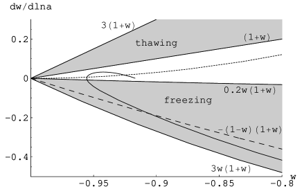
Figure 3: The curve of the quintessence model with $U(\phi)=U_{0}(e^{-\phi/2}+e^{-20\phi})$ in the $w^{\prime}-w$ phase space. This curve crosses the the boundary for thawing and freezing fields Caldwell:2005tm and the lower bound $w^{\prime}=-(1-w)(1+w)$ in Scherrer:2005je ; Chiba:2005tj .

In this paper, we have only studied the case that $w_{\phi}$ (and $\widehat{w}_{\phi})$ keeps on decreasing monotonously, from which the inequality (13) is obtained. In fact, there are quintessence models in which $w_{\phi}$ is increasing at present. One example is the case with $U(\phi)=U_{0}(e^{-\phi/2}+e^{-20\phi})$ Barreiro:1999zs . In this type of models, $w_{\phi}$ will decrease to a minimum close to $-1$ and then begin to increase. So the boundary for thawing and freezing fields in Caldwell:2005tm will be crossed, as shown in Fig. 3. It can be shown that when

$$\frac{d\ln{(\Gamma-1)}}{d\ln{U}}>\frac{3}{2\epsilon}$$

$\widehat{w}_{\phi}$ will be increasing, so will be $w_{\phi}$. It requires a rapid decrease of $\Gamma$. As $\Gamma$ at early times must be close to 1 to get enough tracking, usually there is a rapid increase of $\Gamma$ at recent times. In this case the lower bound $w^{\prime}>-(1-w)(1+w)$ for quintessence models Scherrer:2005je ; Chiba:2005tj may be crossed too. It is because $w=(w_{b}-2\Gamma+2)/(2\Gamma-1)$ will no longer be larger than $w_{\phi}$ if the increase of $\Gamma$ is too fast. It can be seen in Fig. 3 that the line of $w^{\prime}\sim w$ with the double exponential potential is very close to the strict lower bound $w^{\prime}>3w(1+w)$ given in Caldwell:2005tm . For this type of potential, as $w_{\phi}$ and $\widehat{w}_{\phi}$ are increasing, there is an inequality similar to (13):

$$\widehat{w}_{\phi}>w_{\phi},~{}~{}~{}~{}\widehat{\Omega}_{\phi}>\Omega_{\phi}$$ (20)

This inequality can be used to constrain $U(\phi)$ from conditions on ($w_{de},\Omega_{de}$). The methods used in this paper can also be extended to Phantom and K-essence models.

References

(1)
P. J. Steinhardt, L. M. Wang and I. Zlatev,
Phys. Rev. D 59 (1999) 123504
[arXiv:astro-ph/9812313].
(2)
R. J. Scherrer,
Phys. Rev. D 73 (2006) 043502
[arXiv:astro-ph/0509890].
(3)
T. Chiba,
Phys. Rev. D 73 (2006) 063501
[arXiv:astro-ph/0510598].
(4)
S. Lee,
arXiv:astro-ph/0604602.
(5)
A. G. Riess et al. [Supernova Search Team Collaboration],
Astron. J. 116 (1998) 1009
[arXiv:astro-ph/9805201].
(6)
A. G. Riess et al. [Supernova Search Team Collaboration],
Astrophys. J. 607 (2004) 665
[arXiv:astro-ph/0402512].
(7)
A. G. Riess et al.,
Astrophys. J. 659 (2007) 98
[arXiv:astro-ph/0611572].
(8)
D. N. Spergel et al. [WMAP Collaboration],
Astrophys. J. Suppl. 148 (2003) 175
[arXiv:astro-ph/0302209].
(9)
E. Komatsu et al. [WMAP Collaboration],
Astrophys. J. Suppl. 180 (2009) 330
[arXiv:0803.0547 [astro-ph]].
(10)
R. A. Daly and S. G. Djorgovski,
Astrophys. J. 612 (2004) 652
[arXiv:astro-ph/0403664].
(11)
C. Mignone and M. Bartelmann,
arXiv:0711.0370 [astro-ph].
(12)
S. Sullivan, A. Cooray and D. E. Holz,
JCAP 0709 (2007) 004
[arXiv:0706.3730 [astro-ph]].
(13)
R. Lazkoz and E. Majerotto,
JCAP 0707 (2007) 015
[arXiv:0704.2606 [astro-ph]].
(14)
E. J. Copeland, M. Sami and S. Tsujikawa,
Int. J. Mod. Phys. D 15 (2006) 1753
[arXiv:hep-th/0603057].
(15)
A. Mantz, S. W. Allen, H. Ebeling and D. Rapetti,
Mon. Not. Roy. Astron. Soc. 387 (2008) 1179
[arXiv:0709.4294 [astro-ph]].
(16)
C. R. Watson and R. J. Scherrer,
Phys. Rev. D 68 (2003) 123524
[arXiv:astro-ph/0306364].
(17)
S. Bludman,
Phys. Rev. D 69 (2004) 122002
[arXiv:astro-ph/0403526].
(18)
I. Zlatev, L. M. Wang and P. J. Steinhardt,
Phys. Rev. Lett. 82 (1999) 896
[arXiv:astro-ph/9807002].
(19)
R. R. Caldwell and E. V. Linder,
Phys. Rev. Lett. 95 (2005) 141301
[arXiv:astro-ph/0505494].
(20)
P. Brax and J. Martin,
Phys. Rev. D 61 (2000) 103502
[arXiv:astro-ph/9912046].
(21)
T. Barreiro, E. J. Copeland and N. J. Nunes,
Phys. Rev. D 61 (2000) 127301
[arXiv:astro-ph/9910214].