INSTABILITIES IN ELASTOMERS
AND IN SOFT TISSUES

Abstract

Biological soft tissues exhibit elastic properties which can be dramatically different from rubber-type materials (elastomers). To gain a better understanding of the role of constitutive relationships in determining material responses under loads we compare three different types of instabilities (two in compression, one in extension) in hyperelasticity for various forms of strain energy functions typically used for elastomers and for soft tissues. Surprisingly, we find that the strain-hardening property of soft tissues does not always stabilize the material. In particular we show that the stability analyses for a compressed half-space and for a compressed spherical thick shell can lead to opposite conclusions: a soft tissue material is more stable than an elastomer in the former case and less stable in the latter case.

1 Introduction

Elastic materials under external loads may exhibit various responses depending on their geometry, loads, and elastic properties. For large deformations or for inhomogeneous and anisotropic materials as found in biological tissues, these responses are best described in the theory of finite deformations [1]. In hyperelasticity, material properties are specified by a strain-energy function and there is to date a large literature on the derivation and/or fitting of various forms of strain-energy functions [2, 3] for rubber-type materials (referred to as elastomers). The corresponding theory for biological soft tissues is more recent and is not as well established. Nevertheless, there are a few standard forms of strain-energy functions used to model the elastic responses of soft tissues. It has long been emphasized by various authors that soft tissues with their dramatic properties under extension behave differently than elastomers and that in many physiological systems (such as heart, arteries, skin, scalp, etc.) these properties are tuned to achieve specific mechanical goals vital for normal function and regulation [4]. A particularly revealing way to understand the differences between elastomers and soft tissues is to push the material to its extreme by bringing it to a point where a given configuration becomes unstable, and to compare various instabilities for different geometries. Here, we consider three prototype instabilities generated by external loads in an incompressible isotropic elastic body made out of either an elastomer or a biological soft tissue material.

We look in turn at the instabilities generated when a half-space is compressed (Section 3.1), when a spherical membrane shell is inflated (Section 3.2), and when a spherical shell with arbitrary thickness is compressed (Section 3.3). These and other types of instabilities of nonlinear elasticity have been reviewed in an article by Gent [5] where background literature can be found. For the purpose of comparison, we adopt four different strain energy functions which are popular in literature on elastomers and on soft tissues namely, the Mooney-Rivlin model, the Fung model, the Gent model, and the one-term Ogden model. We find that soft tissues behave differently from elastomers when it comes to stability analysis. For instance half-spaces made of soft tissues are stable in compression, whereas half-spaces made of elastomers always possess a critical stretch beyond which surface instabilities develop. Similar conclusions are drawn for inflation instabilities of spherical membrane shells. However, thick-walled spherical shells are found more unstable in compression when made of soft tissues than when made of elastomers. The notion of a material being more or less stable than another one used in this paper is in terms of the critical strains where the material becomes unstable and not in terms of critical stresses or external loads. The general conclusion is that caution must be exercised when choosing an appropriate model for an elastomer or for a soft tissue, because their behaviours with respect to instabilities are not interchangeable. The next Section recalls the basic underlying equations, see Ogden [1], for instance.

2 General set-up

2.1 Static equilibrium

The deformation of the material body is given by $\mathbf{x}=\boldsymbol{\chi}(\mathbf{X})$ where $\mathbf{X}$ and $\mathbf{x}$ describe the material coordinates of a point in the reference configuration and in the current configuration, respectively. Let $\mathbf{F}=\partial\mathbf{x}/\partial\mathbf{X}$ be the deformation gradient. We consider a hyperelastic incompressible body, so that there exists a strain-energy function $W=W(\mathbf{F})$ such that the Cauchy stress tensor $\mathbf{T}$, specifying the stress in the body after deformation, is related to the deformation by

$$\mathbf{T}=\mathbf{F}\dfrac{\partial W}{\partial\mathbf{F}}-p\mathbf{1},$$ (1)

where $p$ is a Lagrange multiplier associated with the internal constraint of incompressibility. The equation for mechanical equilibrium in the absence of body forces is

$$\text{div }\mathbf{T}=\mathbf{0},$$ (2)

where div denotes the divergence operator in the current configuration. Equation (2) provides, through the constitutive relationship (1), a system of three equations for the deformation $\mathbf{x}=\boldsymbol{\chi}(\mathbf{X})$. The boundary conditions are imposed by prescribing the tractions $\mathbf{Tn}$ at the boundary, where $\mathbf{n}$ is the outward unit vector normal to the boundary.

2.2 Strain-energy functions

Many different general functional forms have been proposed or derived to model the response of elastic materials under loads [2, 3, 6]. Here, for comparison purposes, we choose some typical functions that have been proposed to model either elastomers or soft tissues. Since we focus on the role of the strain energy functions in instability and not on the role of possible inhomogeneities or anisotropies, we restrict our attention to homogeneous isotropic materials. We write the energy either in terms of the principal stretches $\lambda_{1}$, $\lambda_{2}$, $\lambda_{3}$ (the square roots of the principal values of $\mathbf{F}\mathbf{F}^{\text{T}}$) or, equivalently for incompressible solids, in terms of the first two principal invariants of the Cauchy-Green strain tensors, given by

$$I_{1}=\lambda_{1}^{2}+\lambda_{2}^{2}+\lambda_{3}^{2},\quad I_{2}=\lambda_{2}^{2}\lambda_{3}^{2}+\lambda_{3}^{2}\lambda_{1}^{2}+\lambda_{1}^{2}\lambda_{2}^{2}.$$ (3)

Here, we limit our investigation to a few key models that capture specific features and are widely used (See Table 1). The main feature of interest for comparison is the strain-stiffening property exhibited by many biological soft tissues. This can be modelled either by algebraic power dependence (one-term Ogden model), by exponential behaviour (as in the popular Fung model), or by limited chain extensibility (Gent model [7, 8, 9]). We write these three models with a single parameter ($\nu$, $\alpha$, $\beta$, respectively) such that the classical neo-Hookean model is obtained in the limits $\nu\to 2$, $\alpha\to 0$, or $\beta\to 0$. Additionally, we also use the classical Mooney-Rivlin strain-energy density, often used to model elastomers; however, experimental values for the material parameter $\mu$ vary widely in the literature and no typical range of values was found.

Name	Definition	soft tissues	elastomers	Ref.
neo-Hookean	$W_{\textrm{nh}}=\frac{1}{2}(I_{1}-3)$
Mooney-Rivlin	$W_{\textrm{mr}}=\dfrac{(I_{1}-3)+\mu(I_{2}-3)}{2(1+\mu)}$
1-term Ogden	$W_{\textrm{og}}=\dfrac{2}{\nu^{2}}(\lambda_{1}^{\nu}+\lambda_{2}^{\nu}+\lambda_{3}^{\nu}-3)$	$\nu\geq 9$	$\nu\approx 3$	[10, 11]
Fung	$W_{\textrm{fu}}=\dfrac{1}{2\alpha}[\text{e}^{\alpha(I_{1}-3)}-1]$	$3<\alpha<20$		[12, 13]
Gent	$W_{\textrm{ge}}=-\dfrac{1}{2\beta}\ln[1-\beta(I_{1}-3)]$	0.4 $<\beta<$3	$0.005<\beta<0.05$	[5, 7, 14, 15]

Table 1: A list of strain-energy functions. Note that the materials share the same infinitesimal shear modulus, which without loss of generality was taken equal to one. The limits $\mu\to 0$, $\alpha\to 0$, $\beta\to 0$, $\nu\to 2$ all lead to the neo-Hookean strain-energy.

3 Instability

We focus on two types of instabilities. One type is related to the notion of limit-point instability, which typically occurs when a balloon is inflated. At first, the balloon is difficult to inflate, and then it may happen that its radius increases dramatically and rapidly, with little or no effort to produce. Here balloons made of elastomers behave completely differently from balloons made of biological soft tissues, as Osborne [16] first observed in 1909, comparing “children’s toys balloons” to “hollow viscera” (dog bladders). This instability is investigated in Section 3.2.

The second type of instability considered in this paper is related to the notion of bifurcation. Bifurcation occurs at values of the material and deformation parameters for which there exist solutions to the incremental equations of equilibrium in the neighbourhood of a finite solution. In other words, the onset of instability is indicated by the existence of adjacent equilibria under the same loading. To investigate that type of instabilities, we consider first a finite deformation $\boldsymbol{\chi}^{(0)}(\mathbf{X})$ and then superimpose an incremental [17] deformation $\boldsymbol{\chi}^{(1)}(\mathbf{x})$ as follows

$$\boldsymbol{\chi}=\boldsymbol{\chi}^{(0)}+\epsilon\boldsymbol{\chi}^{(1)},$$ (4)

where $\epsilon$ is a small parameter. It follows that the deformation gradient is now

$$\mathbf{F}=\partial\boldsymbol{\chi}/\partial\mathbf{X}=\left(\mathbf{1}+\epsilon\mathbf{F}^{(1)}\right)\mathbf{F}^{(0)},$$ (5)

where $\mathbf{F}^{(1)}=\partial\boldsymbol{\chi}^{(1)}/\partial\mathbf{x}$ is expressed in the current configuration. Accordingly, we expand the Cauchy stress tensor in $\epsilon$ as

$$\mathbf{T}=\mathbf{T}^{(0)}+\epsilon\mathbf{T}^{(1)}+\mathrm{O}(\epsilon^{2}),$$ (6)

say, and the constitutive relationship to obtain to zeroth and first orders,

$$\mathbf{T}^{(0)}=\mathbf{F}^{(0)}\dfrac{\partial W}{\partial\mathbf{F}^{(0)}}-p^{(0)}\mathbf{1},\quad\mathbf{T}^{(1)}=\boldsymbol{\mathcal{L}}\,\mathbf{F}^{(1)}+\mathbf{F}^{(1)}\mathbf{F}^{(0)}\dfrac{\partial W}{\partial\mathbf{F}^{(0)}}-p^{(1)}\mathbf{1},$$ (7)

where $p=p^{(0)}+\epsilon p^{(1)}$, $\boldsymbol{\mathcal{L}}$ is the fourth-order tensor of instantaneous elastic moduli, defined by

$$\boldsymbol{\mathcal{L}}\,\mathbf{F}^{(1)}=\mathbf{F}^{(0)}\dfrac{\partial^{2}W}{\partial\mathbf{F}^{(0)}\partial\mathbf{F}^{(0)}}\mathbf{F}^{(1)}\mathbf{F}^{(0)},$$ (8)

and the derivatives of $W$ are evaluated on $\mathbf{F}^{(0)}$; see Ogden [1] for details. Then the stability analysis proceeds by expanding the equation for mechanical equilibrium (2) to first order in $\epsilon$, that is

$$\text{div }\mathbf{T}^{(1)}=\mathbf{0}.$$ (9)

In some cases, the geometry of the problem and the deformations considered are simple enough so that the condition for instability related to the existence of solutions for Equation (9) can be written in terms of $W$ and the $\lambda_{i}$.

We now consider different geometries and our four different strain energy functions, to study three prototype instabilities.

3.1 The half-space in compression

The simplest type of bifurcation is obtained by considering an incompressible hyperelastic half-space with a free surface, under pure homogeneous static deformation with principal stretch ratios $\lambda_{1},\lambda_{2},\lambda_{3}$ [17, 18]. The corresponding instability is then assumed to correspond to the appearance of wrinkles on the free surface, once a critical compressive stretch ratio is reached.

Let $\lambda_{2}$ be the stretch ratio in the direction normal to the free surface. A plane pre-strain is associated with deformations such that $\lambda_{3}=1$ (axial compression), whereas equi-biaxial pre-strains are obtained for either $\lambda_{1}=\lambda_{3}$ (tangential compression) or for $\lambda_{2}=\lambda_{3}$ (normal compression). It follows from the incompressibility condition that $\lambda_{1}\lambda_{2}\lambda_{3}=1$ and therefore we have

$$\lambda_{2}=\lambda_{1}^{n}\quad\left\{\begin{array}[]{ll}n=-1/2&\textrm{normal\ compression},\\ n=-1&\textrm{axial\ compression},\\ n=-2&\textrm{tangential\ compression}.\end{array}\right.$$ (10)

Now, the half-space is occupied with an incompressible hyperelastic material characterized by $W=W(\lambda_{1},\lambda_{2},\lambda_{3})$. It becomes unstable and develops surface instability for critical principal stretch ratios such that [19, 20]

$$\lambda_{2}\left[W_{1}+(2-{\lambda_{2}\over\lambda_{1}})W_{2}\right]+\lambda_{1}^{2}W_{11}-2\lambda_{1}\lambda_{2}W_{12}+\lambda_{2}^{2}W_{22}=0,$$ (11)

where $W_{i}=\partial W/\partial\lambda_{i}$, $W_{ij}=\partial^{2}W/(\partial\lambda_{i}\partial\lambda_{j})$.

We start with the classical elastomer modelled by the Mooney-Rivlin energy $W_{\mathrm{mr}}$ from Table 1. Application of the previous criterion in this case leads to a universal condition (independent of $\mu$) [20]:

$$\lambda_{1}^{n+2}+3\lambda_{1}^{2n+1}-\lambda_{1}^{3n}+\lambda_{1}^{3}=0.$$ (12)

Depending on $n$, we obtain the classical values for the critical compression ratio of instability, for a half-space made of a material with the Mooney-Rivlin (or of course, the neo-Hookean) strain energy function. Green and Zerna [18] found $(\lambda_{1})_{\text{cr}}=0.66614$ under tangential compression ($n=-2$); Biot found $(\lambda_{1})_{\text{cr}}=0.54369$ under axial compression ($n=-1$) and $(\lambda_{1})_{\text{cr}}=0.44375$ under normal ($n=-1/2$) compression.

Next we turn to the popular Fung strain energy for biological soft tissues. We take $W=W_{\textrm{fu}}$ in (11) and obtain after simplification the following bifurcation condition:

$$\lambda_{1}^{n+2}+3\lambda_{1}^{2n+1}-\lambda_{1}^{3n}+\lambda_{1}^{3}+2\alpha(\lambda_{1}^{5}-2\lambda_{1}^{3+2n}+\lambda_{1}^{4n+1})=0.$$ (13)

For $n=-1$ or $n=-2$, there is a corresponding critical value $\alpha_{-1}=1/2$, or $\alpha_{-2}\approx 0.1644$, respectively, after which the bifurcation criterion has no positive real root, see Fig. 1. We conclude that a semi-infinite solid made of a Fung material, under either axial or tangential compression, is always stable for realistic physiological values of the parameters (say $\alpha>1/2$). For $n=-1/2$ (normal biaxial compression), the criterion has a positive real root for all $\alpha$, which however decreases rapidly toward zero, see Fig. 1; hence for $\alpha>3$, the half-space can be compressed by more than 97 % before the bifurcation criterion is met.

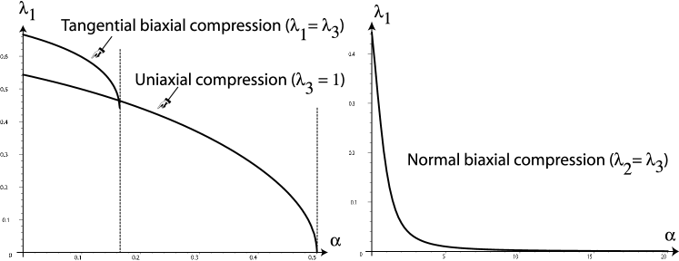
Figure 1: Critical values of the stretch ratio $\lambda_{1}$ for the instability of a Fung elastic half-space characterized by a stiffness-hardening parameter $\alpha$.

Next, we consider the Gent strain energy, originally proposed for rubber [7] but most successfully transposed to the modelling of strain-hardening soft tissues. We take $W=W_{\textrm{ge}}$ in (11) and obtain after simplification the following bifurcation condition,

$$\lambda_{1}^{n-1}+3\lambda_{1}^{2n-2}-\lambda_{1}^{3n-3}+1\\ +\beta(3\lambda_{1}^{n-1}-2\lambda_{1}^{n+1}-11\lambda_{1}^{2n}-\lambda_{1}^{4n-2}+9\lambda_{1}^{2n-2}+\lambda_{1}^{5n-3}+\lambda_{1}^{3n-1}-3\lambda_{1}^{3n-3}+3)=0.$$ (14)

For $n=-1$, $n=-2$, and $n=-1/2$, there is a critical value $\beta_{-1}\approx 0.122$, $\beta_{-2}\approx 0.06$, and $\beta_{-1/2}\approx 0.170$ after which the bifurcation criterion has no positive real root, see Fig. 2. We conclude that a Gent elastic half-space under axial, tangential, or normal compression can become unstable for the parameters values used for elastomers ($0.005<\beta<0.05$) but is always stable for realistic physiological values of soft tissue parameters ($0.4<\beta<3$).

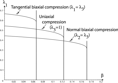
Figure 2: Critical values of the stretch ratio $\lambda_{1}$ for the surface instability of a Gent material characterized by a stiffness-hardening parameter $\beta$.

Finally we use the one-term Ogden model, for which the bifurcation condition reads

$${\lambda_{{1}}}^{n+\nu}+{\lambda_{{1}}}^{n\nu+1}-{\lambda_{{1}}}^{n\left(1+\nu\right)}-{\lambda_{{1}}}^{1+\nu}+\nu\left({\lambda_{{1}}}^{1+\nu}+{\lambda_{{1}}}^{n\nu+1}\right)=0.$$ (15)

The left hand-side of this equation is equal to $-1$ for $\lambda_{1}=0$ and to $2\nu$ for $\lambda_{1}=1$. Therefore, it admits a real root for all positive values of $\nu$ and for all values of $n$. Fig. 3 shows the dependence of the critical compressive stretch ratios on the material parameter $\nu$.

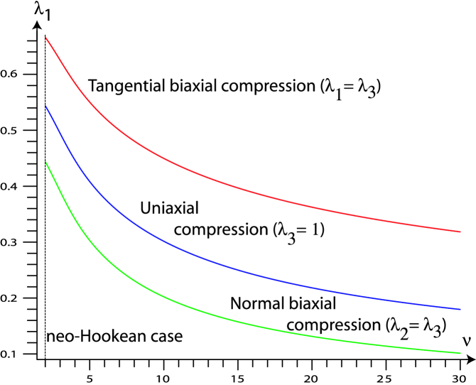
Figure 3: Critical values of the stretch ratio $\lambda_{1}$ for the instability of an Ogden elastic half-space characterized by a stiffness-hardening parameter $\nu$.

3.2 The thin shell in extension

Here we consider a spherical shell subject to an internal pressure $P$. Let $A$, $B$, $R$ denote the inner radius, the outer radius, and the radial position of a material surface in the reference configuration, respectively. Let $a$, $b$, $r$ be the positions of the corresponding material points in the current configuration. In the case of thin shells, we look for a limit-point instability, that is conditions under which the curve $P=P(\lambda_{a})$ has a maximum. When the shell is close to that point, a small increase in pressure can result in a large, sudden increase in radius; this phenomenon is familiar to those who have blown up party balloons.

Before we study the case of thin shells, we consider the radial deformation of a shell under uniform hydrostatic pressure (applied inside or outside). We use spherical coordinates, in which the radial deformation is simply $r=r(R)$, with deformation gradient

$$\mathbf{F}=\mathrm{diag}(r^{\prime},r/R,r/R),$$ (16)

where the prime denotes differentiation with respect to $R$. Since the material is incompressible its volume is preserved and

$$R^{3}-A^{3}=r^{3}-a^{3},\quad R^{3}-B^{3}=r^{3}-b^{3},$$ (17)

which leads to

$$1-\lambda_{a}^{3}=\dfrac{R^{3}}{A^{3}}(1-\lambda^{3})=\dfrac{B^{3}}{A^{3}}(1-\lambda_{b}^{3}),$$ (18)

where $\lambda=r/R$, $\lambda_{a}=a/A$, $\lambda_{b}=b/B$. We denote the non-vanishing components of $\mathbf{T}$ by $t_{1}=T_{11}$ (radial stress), and $t_{2}=T_{22}=T_{33}$ (hoop stress). Then the stress-strain relation (1) reads

$$t_{1}={\lambda_{1}}W_{1}-p,\quad t_{2}={\lambda_{2}}W_{2}-p.$$ (19)

The only non-vanishing equation for mechanical equilibrium (2) in the current configuration is

$${\partial t_{1}\over\partial r}+{2\over r}(t_{1}-t_{2})=0,$$ (20)

and a closed equation for $t_{1}$ is obtained by introducing the auxiliary function $\widehat{W}(\lambda)=W(\lambda^{-2},\lambda,\lambda)$:

$${\partial t_{1}\over\partial r}={\lambda\over r}\widehat{W}^{\prime}(\lambda).$$ (21)

As a function of the circumferential stretch $\lambda$, we have

$${\partial t_{1}\over\partial\lambda}={\widehat{W}^{\prime}(\lambda)\over 1-\lambda^{3}}.$$ (22)

For a shell under internal pressure $P$, the boundary conditions are given by $t_{1}(\lambda_{a})=-P$ and $t_{1}(\lambda_{b})=0$. Integrating (22), we find [21]

$$t_{1}(\lambda)=\int_{\lambda_{b}}^{\lambda}{\widehat{W}^{\prime}(\lambda)\over 1-\lambda^{3}}d\lambda,\quad\text{ and }\quad P=\int_{\lambda_{a}}^{\lambda_{b}}{\widehat{W}^{\prime}(\lambda)\over 1-\lambda^{3}}d\lambda.$$ (23)

Recall that by (18), $\lambda_{b}$ depends on $\lambda_{a}$, so that this latter equation is a relation for $P$ as a function of $\lambda_{a}$; it can be inverted to give the displacement $r=r(R)$ through (18).

Now, a limit-point instability [22, 23, 24, 25, 26, 27] occurs when there is a loss of monotonicity of the function $t_{1}(\lambda_{b})$ as a function of $\lambda_{a}$, that is when the pressure-stretch curve has a a local maximum.

For thin shells, the analysis proceeds by considering the stress to first order in the small parameter $\delta=(B-A)/A$, measuring the thickness of the shell (see for instance Haughton and Ogden [21] or Beatty [28]). Before we proceed with the analysis of thin shells, it is of interest to understand the effect of shell thickness on the instability. To do so, we use the mean-value theorem and the connections (18) to expand (23) to second order in $\delta$. We find

$$t_{1}(\lambda)=\delta{\widehat{W}^{\prime}(\lambda)\over\lambda^{2}}+{\delta^{2}\over 2\lambda^{4}}\left[{\lambda^{3}-2\over\lambda}\widehat{W}^{\prime}(\lambda)-(\lambda^{3}-1)\widehat{W}^{\prime\prime}(\lambda)\right]+{\mathrm{O}}(\delta^{3}),$$ (24)

where $\lambda$ is the position of the inner radius (see Ogden [1, p.285] for the first-order expansion). Since the shell wall-thickness is assumed small, this relation also describes the stress field at every point in the shell.

A limit-point instability occurs for $\lambda_{\text{cr}}$ such that $t_{1}^{\prime}(\lambda_{\text{cr}})=0$. Thus we first differentiate (24) with respect to $\lambda$. Then writing $t_{1}^{\prime}=0$ at order ${\mathrm{O}}(\delta)$, we recover the classical critical circumferential stretch for thin shells [21]: it is $\lambda_{0}$ (say), the smallest solution larger than one of

$$\widehat{W}^{\prime\prime}(\lambda_{0})\lambda_{0}-2\widehat{W}^{\prime}(\lambda_{0})=0.$$ (25)

Next, to explore the dependence of the critical stretch with thickness, we expand $\lambda_{\text{cr}}$ to first order in $\delta$ as $\lambda_{\text{cr}}=\lambda_{0}+\lambda_{\text{cr}}^{(1)}\delta+{\mathrm{O}}(\delta^{2})$, say. Then writing $t_{1}^{\prime}=0$ at order ${\mathrm{O}}(\delta^{2})$, and making use of (25), we find that $\lambda_{\text{cr}}^{(1)}$ is given by the surprisingly simple equation: $\lambda_{0}^{3}-2\lambda_{\text{cr}}^{(1)}\lambda_{0}^{2}-1=0$. It follows that

$$\lambda_{\text{cr}}=\lambda_{0}+{\lambda_{0}^{3}-1\over 2\lambda_{0}^{2}}\delta+{\mathrm{O}}(\delta^{2}).$$ (26)

The first order correction (26) shows that universally (independently of the constitutive relation), the critical stretch of limit-point instability increases with thickness for thin shells. In other words, making a spherical membrane slightly thicker always makes it more stable in inflation, whatever it is made of. Higher-order corrections depend explicitly on the choice of $W$ and no universal result is available. From now on, we focus on membrane shells and neglect the corrections due to $\delta$ (hence, $\lambda_{\text{cr}}$ is now identified with $\lambda_{0}$ given by (25)).

The limit-point instability is readily found for a neo-Hookean thin shell, for which $\widehat{W}(\lambda)=2\lambda^{2}+\lambda^{-4}-3$, as [28] $\lambda_{\text{cr}}=7^{1/6}$ (the neo-Hookean curve $t_{1}(\lambda)$ is shown as the limiting case in Fig. 4). Past this critical value, the membrane continues stretching with reduced pressure. For certain materials, the pressure-stretch curve may present a maximum, followed by a minimum; in that case, once the maximum is reached, and the pressure is increased, the stretch will “jump” to a significantly higher value. This phenomenon is illustrated on Fig. 4 by the horizontal dotted line; it is called an inflation jump. Note that first, a limit-point instability is of course necessary for an inflation jump to occur.

We can now investigate the existence of limit-point instability and of inflation jump in strain-hardening materials. This analysis has been performed by various authors who noted that the limit-point instability disappears as the strain-hardening parameter is increased [1, 10, 28, 29]. Here, we review and expand such results and compute the exact values of the parameters where such instabilities disappear.

We start with a Mooney-Rivlin material and observe that as $\mu$ increases to $\mu_{\text{cr}}$ the limit-point disappears and the curve $t_{1}(\lambda)$ becomes strictly increasing. This critical point is found by solving $t_{1}^{\prime}=t_{1}^{\prime\prime}=0$, which gives

$$\mu_{\text{cr}}=\dfrac{2\sqrt{11}-3}{5(19+6\sqrt{11})^{1/3}}\simeq 0.21446,\quad\lambda_{\text{cr}}=(19+6\sqrt{11})^{1/6}\simeq 1.84073.$$ (27)

The situation is similar for Fung materials (see Fig. 4), where we can readily identify the critical values of the parameters:

$$\alpha_{\text{cr}}={1\over 48}\,{\frac{\left(92+12\,\sqrt{65}\right)^{2/3}\left(3+\sqrt{65}\right)}{57+7\,\sqrt{65}}}\simeq 0.06685,$$ (28)

$$\lambda_{\text{cr}}={1\over\sqrt{2}}(92+12\sqrt{65})^{1/6}\simeq 1.69355.$$ (29)

Hence when $\alpha>0.067$, as is the case for soft biological tissues, there are no limit-point instabilities [28], in accordance with Osborne’s early observations [16].

For Gent materials, we find that the limit-point instabilities disappear when $\beta>\beta_{\text{cr}}$, given by

$$\beta_{\text{cr}}={1\over 3}\,{\frac{\left(10+\sqrt{93}\right)^{2/3}\left(3+\sqrt{93}\right)}{315+33\,\sqrt{93}-\left(10+\sqrt{93}\right)^{2/3}\left(3+\sqrt{93}\right)}}\simeq 0.05669,$$ (30)

and the corresponding circumferential stretch is

$$\lambda_{\text{cr}}=(10+\sqrt{93})^{1/6}\simeq 1.64262.$$ (31)

For instance, Gent [26] found limit-point instabilities (and inflation jumps) for inflated rubber shells with $\beta=0.01$ and $\beta=0.03$. On the other hand, Horgan and Saccomandi [15] estimated that $\beta\approx 0.44$ for the aorta of a 21-year-old male and that $\beta\approx 2.4$ for the (stiffer) aorta of a 70-year-old male, and clearly, there are no limit-point instabilities in those cases (Note that the pressure-stretch curves for Gent materials are almost identical to the ones shown for the Fung energy and are not shown here.)

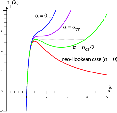
Figure 4: Pressure-stretch curve for a Fung material. The limit $\alpha=0$ is the neo-Hookean material. When $0<\alpha<\alpha_{\text{cr}}$, the system exhibits a limit-point instability and an inflation jump (see dotted line when $\alpha=\alpha_{\text{cr}}/2$). For $\alpha\geqslant\alpha_{\text{cr}}$, the limit-point instability disappears.

The behaviour for an Ogden material is slightly different (Fig. 5). Here again, the limit-point instability disappears rapidly (at $\nu_{c}=3$, below any realistic physiological values). The asymptotic limits for $t_{1}(\lambda)$ as $\lambda\to\infty$ are however different (0, 2, and $\infty$ for $0<\nu<3$, $\nu=3$, and $\nu>3$ respectively). Note finally that there is no inflation jump for any value of $\nu$.

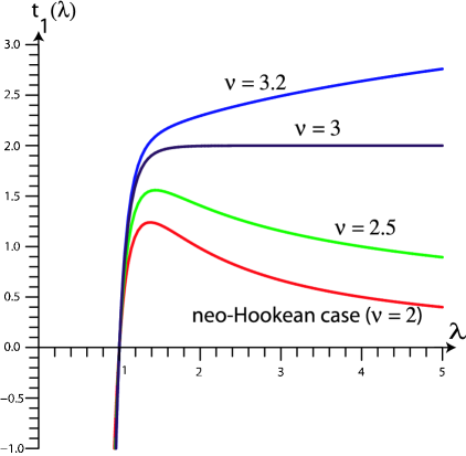
Figure 5: Pressure-stretch curve for a one-term Ogden material. The neo-Hookean material corresponds to $\nu=2$. For $2\leq\nu<3$, the system exhibits a limit-point instability, and $t_{1}(\lambda)\to 0$ as $\lambda\to\infty$. For $\alpha=3$, $t_{1}(\lambda)\to 2$ as $\lambda\to\infty$. For $\nu>3$, $t_{1}(\lambda)\to\infty$ with $\lambda$ and the limit-point instability disappears.

We conclude that for soft biological tissues, the critical parameter values are far below any typical range of physiological values and the limit-point instability is unlikely to be observed. As noted repeatedly by Humphrey and co-workers [29, 30, 31], this observation should be kept in mind when a strain energy function is chosen in numerical simulations of soft tissues, and when designing artificial soft tissues for experiments. The choice of a rubber-like strain energy in the former case, or of an elastomer in the latter case, might lead to instabilities which do not actually exist in the prototype soft tissue.

3.3 The shell under compression

Finally we consider the case of a shell of arbitrary thickness under compression, and analyse its stability with respect to axisymmetric perturbations in the usual $(r,\theta,\varphi)$ spherical coordinates. The stressed state $\boldsymbol{\chi}^{(0)}$ is found explicitly from the computation of the strains and stresses in a spherical shell done in the previous Section. Once this radial stressed state is known we introduce an axisymmetric perturbation $\boldsymbol{\chi}^{(1)}$ which reads

$$\boldsymbol{\chi}^{(1)}=\left[u(r,\theta),v(r,\theta),0\right]^{\mathrm{T}},$$ (32)

where $u$, $v$ are independent of $\varphi$. The gradient $\mathbf{F}^{(1)}$ can be explicitly computed and the condition (9) further simplified by first using the incompressibility constraint and then expanding $u$, $v$ in Legendre polynomials as

$$u(r,\theta)=\sum_{n}U_{n}(r)P_{n}(\cos\theta),\quad v(r,\theta)=\sum_{n}V_{n}(r){d\over d\theta}P_{n}(\cos\theta),$$ (33)

where $P_{n}(\cos\theta)$ are the Legendre polynomials, see [33] for details. After further simplification, a single fourth-order linear ordinary differential equation for $U_{n}$ can be derived

$${d\over dr}\left(C_{3}{d^{3}U_{n}\over dr^{3}}+C_{2}{d^{2}U_{n}\over dr^{2}}+C_{1}{dU_{n}\over dr}\right)+C_{0}U_{n}=0,$$ (34)

where

$$C_{3}=r^{4}{\mathcal{L}_{{1212}}},$$

$$C_{2}=r^{4}{d\over dr}{\mathcal{L}_{{1212}}}+4r^{3}{\mathcal{L}_{{1212}}},$$

$$C_{1}=r^{3}\left(2{d\over dr}{\mathcal{L}_{{1212}}}+t_{1}\right)+r^{2}\bigg{[}(2n^{2}+2n-1)\mathcal{L}_{{1221}}+2n(n+1)\mathcal{L}_{{1122}}$$

$$\qquad\qquad\qquad\qquad-n(n+1)\mathcal{L}_{{1111}}-(n^{2}+n-1)\mathcal{L}_{{2222}}-\mathcal{L}_{{2233}}-\mathcal{L}_{{2121}}\bigg{]},$$

$$C_{0}=(n+2)(n-1)\bigg{[}r^{2}{d^{2}\over dr^{2}}{\mathcal{L}_{{1212}}}$$

$$\qquad\qquad\quad+r{d\over dr}\left(2{\mathcal{L}_{{1212}}}+{\mathcal{L}_{{1221}}}-{\mathcal{L}_{{2121}}}-{\mathcal{L}_{{2222}}}+{\mathcal{L}_{{2233}}}\right)$$

$$\qquad\qquad\qquad\qquad\quad+(n^{2}+n+1){\mathcal{L}_{{2121}}}-{\mathcal{L}_{{1221}}}-2{\mathcal{L}_{{1212}}}+{\mathcal{L}_{{2222}}}-{\mathcal{L}_{{2233}}}\bigg{]}.$$ (35)

The boundary conditions

$$\mathbf{T}^{(1)}\mathbf{n}=\mathbf{0}\quad\mathrm{on\ }r=a,\quad\quad\mathbf{T}^{(1)}\mathbf{n}=-P^{(1)}\mathbf{n}\quad\mathrm{on\ }r=b,$$ (36)

read explicitly

$${d^{3}U_{n}\over dr^{3}}+D_{2}{d^{2}U_{n}\over dr^{2}}+D_{1}{dU_{n}\over dr}+D_{0}U_{n}=0,\quad\quad{d^{2}U_{n}\over dr^{2}}+{2\over r}{dU_{n}\over dr}+{(n^{2}\!+\!n\!-\!2)\over r^{2}}U=0,$$ (37)

where

$$D_{2}={d\over dr}\mathcal{L}_{1212}+{6\over r}\mathcal{L}_{1212},$$

$$D_{1}={1\over r^{2}}\left[-(n+n^{2}+4)\mathcal{L}_{1212}+n(n+1)\mathcal{L}_{1111}-2n(n+1)\mathcal{L}_{1122}+\mathcal{L}_{2233}\right.$$

$$\left.\quad\qquad+(n+n^{2}-1)\mathcal{L}_{2222}-2{d\over dr}\mathcal{L}_{1212}r+2n(n+1)\lambda_{1}W_{1}-\lambda_{2}W_{2}\right],$$

$$D_{0}=-{1\over r^{3}}{(n+2)(n-1)\left[\mathcal{L}_{2233}+2\mathcal{L}_{1212}-\mathcal{L}_{2222}+{d\over dr}\mathcal{L}_{1212}r-\lambda_{2}W_{2}\right].}$$ (38)

The integration of Equation (34) takes place between $r=a$ and $r=b$ for an initial thickness $A/B$ and the problem is to find the value of $a$ such that the boundary conditions are satisfied (the outer radius $b$ is a function of $a$).

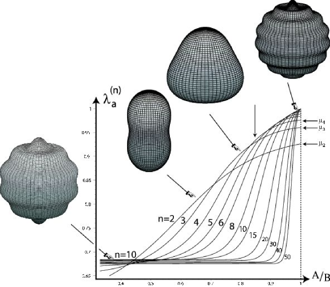
Figure 6: A neo-Hookean shell of inner and outer radii $A$ and $B$ becomes unstable with a critical strain $\lambda_{a}$, the largest possible values of $\lambda_{a}^{(n)}$ (modes $n=$ 2, 3, 4, 5, 6, 8, 10, 15, 20, 30, 40, 50 are shown). The critical mode is the first excited mode. For instance at $A/B=0.85$ (vertical arrow), the critical mode is $n=4$. Examples of shell deformations after the bifurcation are shown for $n=$ 2, 3, 10, 15. Note that the amplitude of the mode has been chosen to show the structure of the solution and is not related to the mechanical problem at hand (the stability analysis is linear and there is no information on the mode amplitude or its sign.)

For this problem we use numerical techniques introduced by Haughton and Ogden [21] and later refined by Fu [32] and by Ben Amar and Goriely [33], among others. For a Fung (exponential) strain energy, we plot the first ten modes at $\alpha=0$ (neo-Hookean), 1, 5, and 10 (strong strain-hardening effect), see Fig. 7. The first graph ($\alpha=0$) corresponds to Fig. 6 and has already been obtained and commented upon in [32, 33] where analytical expansions were derived for the high-number regime and for the thin-walled shell limit. In particular, it was shown in [33] that in the limit $B/A\to 1$ the bifurcation curve for the mode $n$ tends to the first positive root of

$$(n+2)(n-1)\mu^{12}+2(n^{2}+n+7)\mu^{6}-3n(1+n)=0.$$ (39)

The first few roots $\mu_{n}$ are shown in Fig. 6.

Before we consider the effect of strain-hardening it is of importance to further comment on the neo-Hookean shell. The present graph provides additional information. First, it shows that the most unstable mode for thick-walled neo-Hookean shells is mode number 10. Second, the graph makes it clear that at mode 10, the critical stretch tends to a value which is higher than 0.66614 (the compressed half-space critical stretch value, see Section 3.1) as $A/B\to 0$. How is this analysis compatible with the analysis of the neo-Hookean half-space? We expect that in the limit $B\to\infty$ with $A$ constant, the shell should be equivalent to a half-space in tangential bi-axial compression and that we should recover the instability discussed in Section 3.1. In fact, going from a thick-walled spherical shell to a half-space requires a double limit: not only must the shell become infinitely thick (and so $A/B\to 0$), but also the wavelength of the incremental deformation must be infinitesimally small compared to the thickness and radius of the sphere (and so $n\to\infty$); we checked that indeed, $\lambda_{\text{cr}}\to 0.66614$ in these limits.

This last observation turns out to be crucial to interpret correctly the stability of a compressed Fung shell when $\alpha\neq 0$. First, the graphs in Fig. 7 show clearly that compressed spherical shells made of a Fung material are always less stable than shells made of a neo-Hookean material. This trend is further established analytically by determining the exact value for each mode in the limit $A/B\to 1$ which is given by the first positive root of

$$4\alpha^{2}\mu^{20}+2\alpha(n^{2}+n+1)\mu^{18}+(n+2)(n-1)\mu^{16}-16\alpha^{2}\mu^{14}\\ -2\alpha(3n^{2}+3n-2)\mu^{12}+2(n^{2}+n+7)\mu^{10}+20\alpha^{2}\mu^{8}\\ +6\alpha(n^{2}+n-1)\mu^{6}-3n(n+1)\mu^{4}-8\alpha^{2}\mu^{2}-2n\alpha(n+1)=0.$$ (40)

The analysis of these roots reveals that for thin shells the critical bifurcation value for each mode $n$ increases strictly with $\alpha$. In the limit of thick materials we see that Fung shells become unstable at stretch ratios lower than $\lambda_{\text{cr1}}=0.75$ for $\alpha=1$, $\lambda_{\text{cr5}}=0.85$ for $\alpha=5$, $\lambda_{\text{cr10}}=0.91$ for $\alpha=10$. This result might seem counter-intuitive in light of the analysis conducted in Section 3.1 (see also [28]) for surface stability in compression (a neo-Hookean half-space is unstable when $\lambda_{1}<0.66614$ and a Fung half-space is always stable for $\alpha>0.1644$.) However, those lower bounds $\lambda_{\text{cr1}}$, $\lambda_{\text{cr5}}$, $\lambda_{\text{cr10}}$ correspond to low-mode numbers ($n=$ 3, 2, 2 at $\alpha=$ 1, 5, 10, respectively), and not to the high-mode numbers limit necessary to reach the half-space idealization. We further checked that, as $\alpha$ increases, higher modes (say $n>15$) cannot be excited in the limit $A/B\to 0$.

We also conducted numerical investigations (not reproduced here) for the behaviour of shells made of other materials. The results for the Gent and for the one-term Ogden strain energy functions are close to those for Fung materials that is, a shell made of either a Gent or a one-term Ogden material is less stable than a thick shell made of a neo-Hookean material. Again, this is not contradictory with the fact that the Gent and Ogden half-spaces are more stable than the neo-Hookean half-space. The analysis of the half-space is only relevant for high modes.

Finally, we found that a compressed spherical shell made of a Mooney-Rivlin material is slightly more stable than a compressed spherical shell made of a neo-Hookean material (with the same asymptotic limit (39) when $A/B\to 1$. Recall that the Fung, Gent, and Mooney-Rivlin materials are all stiffer in extension (strain-hardening effect) than the neo-Hookean material.

4 Discussion

One cannot help but remark that stability analysis results are difficult to predict in nonlinear elasticity. For instance it is by now well established that thin-walled spherical shells made of Fung materials are extremely stable in inflation. This has been proved in several contexts by Humphrey and his co-workers (see [30] and references therein to earlier work) to refute the hypothesis of an inflation jump instability for the development and rupture of intracranial aneurysms. It might also be commonly accepted that Fung materials are extremely stable in compression, because the half-space stability analysis points clearly in that direction, see Section 3.1. However we demonstrated here that the opposite conclusion is reached for thick spherical shells in compression. Whereas generic strain energy functions may be suitable to describe some properties of materials under loads, special care should be taken when trying to describe instabilities in nonlinear elastic materials.

Figure 7: A shell made of a Fung material of inner and outer radii $A$ and $B$ becomes unstable with a critical strain $\lambda_{a}$, the largest possible values of $\lambda_{a}^{(n)}$ (modes $n=2$ to $10$ are shown).

References

- [1] R. W. Ogden. Non-linear elastic deformations. Dover, New york, 1984.
- [2] M. C. Boyce and E. M. Arruda. Constitutive models for rubber elasticity: a review. Rubber Chem. Technol., 73:504–523, 2000.
- [3] A. P. S. Selvadurai. Deflections of a rubber membrane. J. Mech. Phys. Solids, 54:1093–1119, 2006.
- [4] L. A. Taber. Nonlinear theory of elasticity. World Scientific, New Jersey, 2004.
- [5] A. N. Gent. Elastic instabilities in rubber. Int. J. Non-Linear Mech., 40:165–175, 1995.
- [6] M. S. Sacks. Biaxial mechanical evaluation of planar biological materials. J. Elasticity, 61:199–246, 2000.
- [7] A. Gent. A new constitutive relation for rubber. Rubber Chem. Technol., 69:59–61, 1996.
- [8] C. O. Horgan and G. Saccomandi. A molecular-statistical basis for the Gent constitutive model of rubber elasticity. J. Elasticity, 68:167–176, 2002.
- [9] C. O. Horgan and G. Saccomandi. Constitutive models for compressible nonlinearly elastic materials with limiting chain extensibility. J. Elasticity, 77:123–138, 2004.
- [10] D. K. Bogen and Th A. McMahon. Do cardiac aneurysms blow out? Biophys. J., 27:301–316, 1979.
- [11] O. A. Shergold, N. A. Fleck, and D. Radford. The uniaxial stress versus strain response of pig skin and silicone rubber at low and high strain rates. Int. J. Impact Eng., 32:1384–1402, 2006.
- [12] G. A. Holzapfel, T. C. Gasser, and R. W. Ogden. A new constitutive framework for arterial wall mechanics and a compartaive study of material models. J. Elasticity, 61:1–48, 2000.
- [13] A. Delfino, N. Stergiopulos, J. E. Moore, and J. J Meister. Residual strain effects on the stress field in a thick wall finite element model of the human carotid bifurcation. J. Biomech., 30:777–786, 1997.
- [14] C. O. Horgan and G. Saccomandi. Constitutive modeling of rubber-like and biological materials with limited chain extensibility. Math. Mech. Solids, 7:353–371, 2002.
- [15] C. O. Horgan and G. Saccomandi. A description of arterial wall mechanics using limiting chain extensibility constitutive models. Biomechan. Model Mechanobiol., 1:251–266, 2003.
- [16] W.A. Osborne, The elasticity of rubber balloons and hollow viscera. Proc. Roy. Soc. Lond., B81: 485–499, 1909.
- [17] M. A. Biot. Mechanics of incremental deformation. Wiley, New York, 1965.
- [18] A. E. Green and W. Zerna. Theoretical Elasticity. Dover, New York, 1992.
- [19] M. A. Dowaikh and R. W. Ogden. On surface waves and deformations in a pre-stressed incompressible elastic solid. IMA J. Appl. Math., 44:261–284, 1990.
- [20] M. Destrade. Rayleigh waves and surface stability for Bell materials in compression: comparison with rubber. Q. Jl. Mech. Appl. Math., 56:593–604, 2003.
- [21] D. M. Haughton and R. W. Ogden. On the incremental equations in non-linear elasticity-II. Bifurcation of pressurized spherical shells. J. Mech. Phys. Solids, 26:111–138, 1978.
- [22] J. E. Adkins and R. S. Rivlin. Large elastic deformations of isotropic materials. IX. The deformation of thin shells. Phil. Trans. Roy. Soc. A, 244:505–531, 1952.
- [23] H. Alexander. Tensile instability of initially spherical balloons. Int. J. Engng. Sci, 9:151–162, 1971.
- [24] R. W. Ogden. Large deformation isotropic elasticity - On the correlation of theory and experiment for incompressible rubberlike solids. Proc. Roy. Soc. Lond. A, 326:565–584, 1972.
- [25] Y. C. Chen and T. J. Healey. Bifurcation to pear-shaped equilibria of pressurized spherical membranes. Int. J. Non-Linear Mech., 26:279–291, 1991.
- [26] A. Gent. Elastic instabilities of inflated rubber shells. Rubber Chem. Technol., 72:263–268, 1999.
- [27] I. Müller and H. Struchtrup. Inflating a rubber balloon. Math. Mech. Solids, 7:569–577, 2002.
- [28] M. F. Beatty. Introduction to nonlinear elasticity. In M. M. Carroll and M. Hayes, editors, Nonlinear effects in fluids and solids, pages 13–112. Plenum Press, New York, 1996.
- [29] J. D. Humphrey. Cardiovascular solid mechanics. Cells, tissues, and organs. Springer Verlag, New York, 2002.
- [30] G. David and J. D. Humphrey. Further evidence for the dynamic stability of intracranial saccular aneurysms. J. Biomech., 36:1143–1150, 2003.
- [31] H. W. Haslach and J. D. Humphrey. Dynamics of biological soft tissue and rubber: internally pressurized spherical membranes surrounded by a fluid. Int. J. Non-linear Mech., 39:399–420, 2004.
- [32] Y. Fu. Some asymptotic results concerning the buckling of a spherical shell of arbitrary thickness. Int. J. Non-linear Mech., 33:1111–1122, 1998.
- [33] M. Ben Amar and A. Goriely. Growth and instability in soft tissues. J. Mech. Phys. Solids, 53:2284–2319, 2005.