A condition number analysis of an algorithm for solving a system of polynomial equations with one degree of freedom

Abstract

This article considers the problem of solving a system of $n$ real polynomial equations in $n+1$ variables. We propose an algorithm based on Newton’s method and subdivision for this problem. Our algorithm is intended only for nondegenerate cases, in which case the solution is a 1-dimensional curve. Our first main contribution is a definition of a condition number measuring reciprocal distance to degeneracy that can distinguish poor and well conditioned instances of this problem. (Degenerate problems would be infinitely ill conditioned in our framework.) Our second contribution, which is the main novelty of our algorithm, is an analysis showing that its running time is bounded in terms of the condition number of the problem instance as well as $n$ and the polynomial degrees.

1 Introduction

We consider the problem of finding all zeros of a polynomial function $f:[0,1]^{n+1}\rightarrow\mathbb{R}^{n}$. The zero-set of such a function will, in the generic case, be a 1-dimensional algebraic set. Our algorithm is enumerative in nature, and therefore is feasible only in the case of small values of $n$. We refer to this problem as the single-degree-of-freedom polynomial system problem (SDPS).

Perhaps the most common application of the SDPS problem is finding the intersection of two rational or polynomial surfaces, the so-called surface/surface intersection (SSI) problem. In this case, one is given two polynomials $p_{1},p_{2}$ both mapping $\mathbb{R}^{2}$ to $\mathbb{R}^{3}$ that each parametrize a surfaces. The problem is to find their intersection, i.e., all points $(s,t,u,v)$ in $[0,1]^{4}$ such that $p_{1}(s,t)-p_{2}(u,v)=0$. Other applications arise in robotics and motion planning. A final application is global optimization in which one finds all the local minimizers by constructing a network of paths that connect local minimizers (see, e.g., [14]).

Our proposed algorithm is a hybrid between subdivision and iterative methods. This hybrid idea has been used to solve surface/surface intersection by Koparkar [13] and to solve line/surface intersection by Toth [22]. The approach is to subdivide the domain recursively, discard the subdomains found to contain no solutions, and invoke an iterative method to locate a solution once it is certain that the iterative method converges. The convergence tests used by Toth and Koparkar are both based on contraction mapping and evaluating ranges of functions.

Our first main contribution, detailed in Section 3, is the definition of a condition number for SDPS problems. Intuitively, a problem instance is ill conditioned if it is close to a degenerate instance. A degenerate instance is one in which the Jacobian fails to have full rank at a root. Our condition number is the reciprocal of a quantity related to nearness to degeneracy. It is natural to expect that algorithms would have poorer behavior as the condition number grows larger.

Our algorithm, which is presented in Sections 5–6, is similar to Koparkar’s in that it subdivides the parametric domains of the problem until the subdomains pass certain tests. It uses a bounding volume of a subdomain to exclude any that cannot have a solution. Our convergence test is based on the Kantorovich theorem, which tells us if Newton’s method converges quadratically for the initial point in question in addition to whether it converges at all. For this reason, we can choose to hold off Newton’s method until quadratic convergence is assured. Kantorovich’s theorem is presented in Section 2.

The main feature of our algorithm is that there is a lower bound on the size of the smallest hypercube occurring during the course of the algorithm that depends on the reciprocal condition number of the problem instance and on the polynomial degrees. Because our interest is in the low-dimensional and moderate degree case, we regard the factors depending on the degrees as ‘constants’ and the dependence on the condition number as the interesting feature. This analysis is presented in Section 7. A lower bound on the smallest hypercube size consequently implies an upper bound on the overall running time.

As mentioned above, the SSI problem is a special case of SDPS with $n=3$. Since there are many algorithms for SSI proposed in literature, we discuss here the main advantage of our algorithm as compared to other SSI algorithms. To the best of our knowledge, there is no previous algorithm for SSI in this class whose running time has been bounded in terms of the condition of the underlying problem instance, and we are not sure whether such an analysis is possible for previous algorithms. Indeed, we do not know of any SSI algorithm in the literature that has any a priori bound on the running time. We do know, however, that some algorithms do not have this property—their running time can be arbitrarily large even if the input instance is well conditioned. This is because these algorithms can sometimes create degenerate or nearly degenerate subproblems even though the original input instance is well conditioned. Section 4 shows in details how marching methods based on collinear normal points and Koparkar’s algorithm in particular have the capacity to create bad subproblems from a good instance.

The notion of bounding the running time of an iterative method in terms of the condition number of the instance is an old one, with the most notable example being the condition-number bound of conjugate gradient (see Chapter 10 of [10]). This approach has also been used in interior-point methods for linear programming [9], Krylov-space eigenvalue computation [21], and the line/surface intersection problem [19]. We note that a related problem of computing convex hull of points on a plane is shown to always be well-conditioned [11].

An additional motivation, not pursued further herein, for defining a condition number and condition-aware algorithms like ours is that this creates the possibility of preconditioning. Preconditioning, which has been very successfully applied in numerical linear algebra (see, e.g., [23]), means improving the condition number of an instance via some kind of transformation prior to solving it.

We now define the problem under consideration more precisely by specifying a representation for the input polynomial system. Let $Z_{i,m}(t)$ denote the Bernstein polynomials

$$Z_{i,m}(t)=\frac{m!}{i!(m-i)!}(1-t)^{m-i}t^{i}.$$

We are interested in finding all points $x=\left(x_{1},x_{2},\ldots,x_{n+1}\right)^{T}\in[0,1]^{n+1}$ satisfying

$$f(x)\equiv\sum_{i_{1}=0}^{m_{1}}\cdots\sum_{i_{n+1}=0}^{m_{n+1}}b_{i_{1},\cdots,i_{n+1}}Z_{i_{1},m_{1}}(x_{1})\cdots Z_{i_{n+1},m_{n+1}}(x_{n+1})=0,$$ (1)

where $b_{i_{1},\cdots,i_{n+1}}\in\mathbb{R}^{n}$ $(i_{j}=0,1,\ldots,m_{j})$ denote the coefficients, also known as the control points. Therefore, the problem is specified by the $(m_{1}+1)(m_{2}+1)\cdots(m_{n+1}+1)$ control points. (See a further remark on this matter in Section 9). This form of a multivariate polynomial is sometimes called tensor product Bézier representation: it presumes that the maximum degree of variable $x_{i}$ (separately) is $m_{i}$ for each $i=1,\ldots,n+1$. Note that $f$ is a function that maps $\mathbb{R}^{n+1}$ to $\mathbb{R}^{n}$. Note that this representation would be intractable for a large value of $n$, but, as mentioned earlier, our algorithm is intended for small values such as $n=3$.

The Bernstein basis is known to have better numerical stability for polynomials on the unit interval than the power basis [8, 7], and computation using parametric representation is often much more efficient than other types of surface representations. Furthermore, our algorithm makes direct use of the Bernstein-Bézier representation. In particular, our exclusion test is based on Bézier control points. It should be noted that the algorithm proposed in this article can be generalized to use with parametric surfaces represented by other polynomial bases provided that an appropriate exclusion test is available, and a few other properties hold for the basis. Refer to [19] for a related algorithm for line/surface intersection that can operate on parametric surfaces represented by other polynomial bases.

2 The theorem of Kantorovich

Denote the closed ball centered at $x$ with radius $r>0$ by

$$\bar{B}(x,r)=\{y\in\mathbb{R}^{n}:\left\|y-x\right\|\leq r\},$$

and let $B(x,r)$ denote the interior of $\bar{B}(x,r)$. Kantorovich’s theorem in affinely invariant form, which is valid for any norm, is as follows.

Theorem 2.1 (Kantorovich, affinely invariant form [5, 12]).

Let $f:D\subseteq\mathbb{R}^{n}\rightarrow\mathbb{R}^{n}$ be differentiable in the open convex set $D$. Assume that for some point $x^{0}\in D$, the Jacobian $f^{\prime}(x^{0})$ is invertible with

$$\left\|f^{\prime}(x^{0})^{-1}f(x^{0})\right\|\leq\eta.$$

Let there be a Lipschitz constant $\omega>0$ for $f^{\prime}(x^{0})^{-1}f^{\prime}$ such that

$$\left\|f^{\prime}(x^{0})^{-1}(f^{\prime}(x)-f^{\prime}(y))\right\|\leq\omega\cdot\left\|x-y\right\|\textrm{ for all }x,y\in D.$$

If $h=\eta\omega\leq 1/2$ and $\bar{B}(x^{0},\rho_{-})\subseteq D$, where

$$\rho_{-}=\frac{1-\sqrt{1-2h}}{\omega},$$

then $f$ has a zero $x^{*}$ in $\bar{B}(x^{0},\rho_{-})$. Moreover, this zero is the unique zero of $f$ in $(\bar{B}(x^{0},\rho_{-})\cup B(x^{0},\rho_{+}))\cap D$ where

$$\rho_{+}=\frac{1+\sqrt{1-2h}}{\omega}$$

and the Newton iterates $x^{k}$ defined by

$$x^{k+1}=x^{k}-f^{\prime}(x^{k})^{-1}f(x^{k})$$

are well-defined, remain in $\bar{B}(x^{0},\rho_{-})$, and converge to $x^{*}$. In addition,

$$\left\|x^{*}-x^{k}\right\|\leq\frac{\eta}{h}\left(\frac{(1-\sqrt{1-2h})^{2^{k}}}{2^{k}}\right),k=0,1,2,\ldots$$

We call $x^{0}$ a fast starting point if the quantity $h$ defined above satisfies $h\leq 1/4$ and $\bar{B}(x^{0},\rho_{-})\subseteq D$. In this case, quadratic convergence of the iterates starting from $x^{0}$ is implied.

3 A condition number of a polynomial system with one degree of freedom

In this section we propose a definition for a condition number of the SDPS problem and prove that our condition number is related to the distance from degeneracy. Let $M$ denote the maximum $p$-norm among the control points of $f$ for some $p$. Later on, we will specialize to the infinity norm. It is easy to show that this quantity satisfies the axioms of a norm, so we will write $M$ also as $\|f\|$. Define the condition number of $f$ to be

$$\mathop{\rm{cond}}(f)=M\cdot\max_{x\in[0,1]^{n+1}}\left(\min\left\{{\frac{1}{\left\|f(x)\right\|}},\left\|f^{\prime}(x)^{\dagger}\right\|\right\}\right).$$ (2)

Here, the notation $A^{\dagger}$ means $A^{\dagger}=A^{T}(AA^{T})^{-1}$. In the case that the rank of $A$ is $n$, this corresponds to the Moore-Penrose pseudo-inverse of $A$, typically denoted as $A^{+}$. In general, the Moore-Penrose pseudo-inverse is defined for matrices of all ranks. In this paper, however, we need $A^{\dagger}$ only in the case that $\mathop{\rm{rank}}(()A)=n$; we will take the second factor $\left\|f^{\prime}(x)^{\dagger}\right\|$ of $(\ref{cond_def})$ to be $\infty$ if the rank of $f^{\prime}(x)$ is less than $n$. Similarly, the first factor is taken to be $\infty$ if $f(x)=0$. Note that small condition number means the problem is well-conditioned. Indeed, it follows from $(\ref{eq:fMbound})$ and $(\ref{eq:Mpinvineq})$ below that both terms in the min have a lower bound of $\mbox{const}/M$.

The rationale for this definition is that, as mentioned earlier, a degenerate instance has a point $x$ such that $f(x)=0$ and $\mathop{\rm{rank}}(()f^{\prime}(x))<n$. For such a point, both terms occurring in the min of $(\ref{cond_def})$ are infinity, i.e., the condition number is infinite. Thus, the problem is ill-conditioned if $f(x)$ is close to zero and $f^{\prime}(x)$ is close to rank-deficiency at the same point $x$.

The inclusion of the factor of $M$ makes the definition scale-invariant. Note that $M$ depends on the choice of basis, namely, tensor-product Bernstein-Bézier basis, whereas the other factors in the condition number are basis-independent. The dependence on basis, however, is only up to a scalar factor depending on degree. This is because polynomials are a finite-dimensional vector space, hence all norms are equivalent. We could redefine $M$ in a basis-independent manner as follows:

$$M_{\rm BI}=\max_{x\in[0,1]^{n+1}}\|f(x)\|.$$

It follows from $(\ref{eq:fMbound})$ and $(\ref{theta_eq})$ below that $M_{\rm BI}$ and $M$ differ by a scalar that is bounded in terms of the degrees. The definition $M_{\rm BI}$, however, would be harder to compute in practice.

This condition number is similar to the definition of $\tilde{\kappa}(f)$ of Cucker et al. [3] for the problem of computing isolated roots of polynomial systems $\mathbb{R}^{n}\rightarrow\mathbb{R}^{n}$. Our definition is somewhat simpler than theirs, however, because of the assumption we have imposed that the domain of interest is $[0,1]^{n+1}$ rather than all of $\mathbb{R}^{n+1}$. This simplifying assumption obviates the need for introducing projective space and scaling of coefficients as in [3].

The classical Turing Theorem [2] states that the condition number of a matrix, which bounds the iteration count of the conjugate gradient algorithm, is exactly the reciprocal of the relative distance of the matrix to singularity. Similarly, Shub and Smale show that their condition number for a homogeneous polynomial system is equal to the distance of the system to singularity [17]. We now derive a result showing that our proposed condition number is also related to the distance of an SDPS instance to degeneracy.

Before stating and proving the theorem, we require two well known bounds concerning polynomials in Bernstein-Bézier form:

$$\|f(x)\|\leq\|f\|$$ (3)

for all $x\in[0,1]^{n+1}$. This follows because every value of $f$ over the parametric domain is a convex combination of control points [6]. Next,

$$\|f^{\prime}(x)\|_{\infty}\leq\left\|f^{\prime}\right\|_{\infty}\leq 2(n+1)\max(m_{1},m_{2},\ldots,m_{n+1})\|f\|_{\infty}$$ (4)

for all $x\in[0,1]^{n+1}$. This follows because the control points of a column of $f^{\prime}$ (i.e., a partial derivative of $f$) are finite differences of control points of $f$ multiplied by the degree in the direction of differentiation as in $(\ref{eq:bezderiv1})$. A factor of $2$ comes from the taking of finite differences, and a further factor of $n+1$ arises from the fact that the infinity norm is a sum over rows (not columns) of the derivative. Furthermore, applying the equivalence of norms to $(\ref{eq:fpMbound})$ yields

$$\left\|f^{\prime}\right\|\leq 2\alpha_{n}(n+1)\max(m_{1},m_{2},\ldots,m_{n+1})\|f\|$$ (5)

for any arbitrary $p$-norm, where $\alpha_{n}>0$ is a scalar depending on $n$ and the choice of norm.

Now, finally, we come to the main theorem of this section.

Theorem 3.1.

Let $f:[0,1]^{n+1}\rightarrow\mathbb{R}^{n}$ be a polynomial function of degrees $m=(m_{1},m_{2},\ldots,m_{n+1})$ in its $n+1$ variables, and assume that it is nondegenerate, i.e., there is no $x\in[0,1]^{n+1}$ such that $f(x)=0$ and $\mathop{\rm{rank}}(()f^{\prime}(x))<n$. Then any $\tilde{f}$ satisfying

$$\frac{\|\tilde{f}-f\|}{\|f\|}\leq\frac{c_{m}}{\mathop{\rm{cond}}(f)}$$ (6)

is nondegenerate, where $c_{m}$ is a scalar depending on the degrees and the choice of norm.

Conversely, there exists a degenerate polynomial $\hat{f}$ such that

$$\frac{\|\hat{f}-f\|}{\|f\|}\leq\frac{c_{m}^{\prime}}{\mathop{\rm{cond}}(f)},$$ (7)

where $c_{m}^{\prime}$ is another scalar depending on the degrees.

Remark 1. As mentioned above, the vector and matrix norms appearing in $(\ref{eq:hatfminusf1})$, $(\ref{eq:hatfminusf2})$ may be any of the standard $p$-norms, although later we will specialize to the infinity norm. Inequalities $(\ref{eq:hatfminusf1})$ and $(\ref{eq:hatfminusf2})$ involve the norm of the polynomial function. As mentioned above, we take this to mean the maximum norm control point when written in Bernstein-Bézier form.

Remark 2. Let $\mathcal{D}$ denote the set of degenerate polynomials, that is, those polynomials $f$ such that $\mathop{\rm{cond}}(f)=\infty$. This theorem shows that our condition number is, up to constant factors, the reciprocal distance of $f$ to $\mathcal{D}$ scaled by the norm of $f$. Consider a larger set $\mathcal{D}^{\prime}$ of degenerate polynomials defined as follows. Polynomial $f\in\mathcal{D}^{\prime}$ if there is any point $x$ in $\mathbb{C}^{n+1}$ (not merely $[0,1]^{n+1}$) such that $f(x)=0$ and $f^{\prime}(x)$ is rank deficient. This set $\mathcal{D^{\prime}}$ is an algebraic variety, i.e., the coefficients of such $f$’s are the roots of a polynomial system. This means that we can apply Demmel’s theorem [4] to conclude that the expected logarithm of the condition number of a random instance is modest. (Clearly, the distance of a polynomial $f$ to $\mathcal{D}$ is bounded below by the distance of $f$ to $\mathcal{D}^{\prime}$.) We can also apply the more recent analysis of Bürgisser et al. [1] to show that the ‘smoothed’ condition number [18] is modest, i.e., for any polynomial $f$ (even a degenerate one), if we select a random small perturbation of it, then the resulting polynomial is expected to have a modest logarithmic condition number.

Proof.

Let $\tilde{f}$ satisfy $(\ref{eq:hatfminusf1})$ and let $e=f-\tilde{f}$ (i.e., a polynomial), so that $\|e\|\leq c_{m}\|f\|/\mathop{\rm{cond}}(f)$. Choose an $x\in[0,1]^{n+1}$. By definition of $\mathop{\rm{cond}}(f)$,

$$M\cdot\min(1/\|f(x)\|,\|f^{\prime}(x)^{\dagger}\|)\leq\mathop{\rm{cond}}(f).$$

We take two cases depending on which term achieves the min. First, suppose $M/\|f(x)\|\leq\mathop{\rm{cond}}(f)$. In this case, $\|f(x)-\tilde{f}(x)\|=\|e(x)\|\leq\|e\|\leq c_{m}\|f\|/\mathop{\rm{cond}}(f)$. Assume $c_{m}$ is sufficiently small so that $c_{m}<1/3$. Then

$$\frac{1}{\|\tilde{f}(x)\|} \leq \frac{1}{\|f(x)\|-\|f(x)-\tilde{f}(x)\|}$$

$$\leq \frac{1}{\|f\|/\mathop{\rm{cond}}(f)-c_{m}\|f\|/\mathop{\rm{cond}}(f)}$$

$$\leq 1.5\mathop{\rm{cond}}(f)/\|f\|.$$

In particular, $\tilde{f}(x)\neq 0$.

For the other case, the hypothesis is $\|f\|\cdot\|f^{\prime}(x)^{\dagger}\|\leq\mathop{\rm{cond}}(f)$. We recall that

$$\frac{1}{\sigma_{n}(f^{\prime}(x))\sqrt{n}}\leq\|f^{\prime}(x)^{\dagger}\|_{\infty}\leq\frac{\sqrt{n+1}}{\sigma_{n}(f^{\prime}(x))}$$ (8)

(see [10, (2.3.11) and §5.5.4]), where $\sigma_{n}(\cdot)$ is notation for the $n$th singular value of a matrix. By the equivalence of norms, $(\ref{eq:fromgvl})$ is equivalent to

$$\frac{\delta_{n}}{\sigma_{n}(f^{\prime}(x))\sqrt{n}}\leq\|f^{\prime}(x)^{\dagger}\|\leq\frac{\gamma_{n}\sqrt{n+1}}{\sigma_{n}(f^{\prime}(x))}$$

for any arbitrary $p$-norm, where $\delta_{n}$ and $\gamma_{n}$ are positive constants that depend on $n$ and the choice of norm.

A second fact from numerical linear algebra is that

$$|\sigma_{i}(A)-\sigma_{i}(B)|\leq\|A-B\|_{2}\leq\sqrt{n}\|A-B\|$$

(see [10, (2.3.11) and Cor. 8.6.2]). Combining these facts together with $(\ref{eq:ebound})$ yields

$$\sigma_{n}(\tilde{f}^{\prime}(x)) = \sigma_{n}(f^{\prime}(x)-e^{\prime}(x))$$

$$\geq \sigma_{n}(f^{\prime}(x))-\sqrt{n}\|e^{\prime}\|$$

$$\geq \sigma_{n}(f^{\prime}(x))-2\alpha_{n}\sqrt{n}(n+1)\max(m_{1},\ldots,m_{n+1})\|e\|$$

$$\geq \frac{\delta_{n}}{\sqrt{n}\|f^{\prime}(x)^{\dagger}\|}-\frac{2\alpha_{n}\sqrt{n}(n+1)\max(m_{1},\ldots,m_{n+1})c_{m}\|f\|}{\mathop{\rm{cond}}(f)}$$

$$\geq \frac{\delta_{n}\|f\|}{\sqrt{n}\mathop{\rm{cond}}(f)}-\frac{2\alpha_{n}\sqrt{n}(n+1)\max(m_{1},\ldots,m_{n+1})c_{m}\|f\|}{\mathop{\rm{cond}}(f)}.$$

If we select $c_{m}<\delta_{n}/\left(2\alpha_{n}n(n+1)\max(m_{1},\ldots,m_{n+1})\right)$, then we are assured in this case that $\sigma_{n}(\tilde{f}^{\prime}(x))>0$, i.e., the rank of $\tilde{f}^{\prime}(x)$ is $n$.

Thus, combining the cases, we have shown that for all $x\in[0,1]^{n+1}$, either $\tilde{f}(x)\neq 0$ or the rank of $\tilde{f}^{\prime}(x)$ is at least $n$, thus proving that $\tilde{f}$ is not degenerate.

Next, let us turn to $(\ref{eq:hatfminusf2})$. In this proof, we will drop the prime from $c_{m}^{\prime}$ and indeed will allow $c_{m}$ to denote a constant depending on the degrees that may change from line to line.

Let $x_{0}\in[0,1]^{n+1}$ be the point where the max in $(\ref{cond_def})$ is achieved, and let $k$ be the value of this max, i.e., the value of $\mathop{\rm{cond}}(f)$. This means, first, that $\|f(x_{0})\|\leq M/k$. Second, it means that either (i) $\|f^{\prime}(x_{0})^{\dagger}\|\geq k/M$, or (ii) $\mathop{\rm{rank}}(()f^{\prime}(x_{0}))<n$. Let $A=f^{\prime}(x_{0})$.

If case (i) is true, then by definition of the matrix $p$-norm there exists a unit vector (in the norm under consideration) $r$ such that $\|A^{T}(AA^{T})^{-1}r\|\geq k/M$. Let $q=A^{T}(AA^{T})^{-1}r$, so that $\|q\|\geq k/M$ and $Aq=r$. Let $S=rq^{T}/(q^{T}q)$ (a $n\times(n+1)$ matrix) and define $\hat{f}(x)\equiv f(x)-f(x_{0})-S(x-x_{0})$. In case (ii) (when $\mathop{\rm{rank}}(()f^{\prime}(x_{0}))<n$), define $\hat{f}(x)\equiv f(x)-f(x_{0})$, i.e., take $S=0$, and we do not need $r$ and $q$.

For either case, we now must establish that $\hat{f}$ is a degenerate instance and that inequality $(\ref{eq:hatfminusf2})$ holds.

First, let us establish the degeneracy of $\hat{f}$. Clearly $x_{0}$ is a root of $\hat{f}$. In case (ii), $\hat{f}^{\prime}(x_{0})=f^{\prime}(x_{0})$, a matrix whose rank is less than $n$. In case (i), $\hat{f}^{\prime}(x_{0})=f^{\prime}(x_{0})-S=A-rq^{T}/(q^{T}q)$. We claim that $\hat{f}^{\prime}(x_{0})$ has at least two independent vectors in its null space, which implies that its rank is at most $n-1$. Observe first that $A$, as an $n\times(n+1)$ matrix, must have a nonzero vector $w$ in its null space. Then $w$ is also in the null space of $\hat{f}^{\prime}(x_{0})$ since $Aw=0$ and $q^{T}w=r^{T}(AA^{T})^{-1}Aw=0$. Also, $\hat{f}^{\prime}(x_{0})$ has $q$ in its null space as $\hat{f}^{\prime}(x_{0})q$ evaluates to $Aq-r$. Finally, $q$ and $w$ are independent since $Aw=0$ whereas $Aq=r$, which is not zero. This concludes the argument that $\hat{f}$ is degenerate.

Next, consider $\|\hat{f}-f\|$ appearing in $(\ref{eq:hatfminusf2})$. Let us introduce the following notation for this argument: $\tau$ denotes the polynomial $x\mapsto x-x_{0}$ and $\kappa$ denotes the constant real-valued polynomial 1. With these definitions, $\hat{f}-f=f(x_{0})\kappa+S\tau$. Note that $\|\tau\|\leq c_{m}$ since $\|x_{0}\|\leq 1$. Also, $\|\kappa\|=1$. We have the following chain of inequalities, which applies to case (i). The first line involves norms of polynomials, whereas the remaining lines are norms of vectors and matrices.

$$\|\hat{f}-f\| = \|f(x_{0})\kappa+S\circ\tau\|$$ (9)

$$\leq c_{m}\left(\|f(x_{0})\|+\|S\|\right)$$

$$\leq c_{m}\left(\frac{M}{k}+\|rq^{T}/(q^{T}q)\|\right)$$

$$\leq c_{m}\left(\frac{M}{k}+\|r\|\cdot\|q^{T}/(q^{T}q)\|\right)$$

$$\leq c_{m}\left(\frac{M}{k}+\|r\|\cdot 1/\|q\|\right)$$

$$\leq c_{m}\left(\frac{M}{k}+\|r\|\cdot M/k\right)$$

$$\leq c_{m}\frac{M}{k}.$$

The first line follows from the definition of $\hat{f}$. The second uses the fact that $\|\kappa\|$ and $\|\tau\|$ are bounded by constants. The third line uses the inequality established earlier that $\|f(x_{0})\|\leq M/k$ and also expands the definition of $S$. The fifth line uses the fact that $q^{T}q=\|q\|^{2}_{2}$, and the 2-norm and the $p$-norm under consideration are related by constants depending on $m_{1},\ldots,m_{n+1}$. The last line uses the assumption that $r$ is a unit vector.

For case (ii), $(\ref{eq:hatfminusf_numer})$ also holds since $S=0$, so the result is already established by the third line in the above chain of inequalities. Since the denominator occurring in the left-hand side of $(\ref{eq:hatfminusf2})$ is $M$, and recalling that $k=\mathop{\rm{cond}}(f)$, we see that $(\ref{eq:hatfminusf_numer})$ proves the theorem. ∎

Although the condition number defined by $(\ref{cond_def})$ is scale invariant (i.e., $\mathop{\rm{cond}}(f)\equiv\mathop{\rm{cond}}(cf)$ for $c\neq 0$), it is not affinely invariant. In other words, if $A$ is a nonsingular $n\times n$ matrix, then in general $\mathop{\rm{cond}}(f)\neq\mathop{\rm{cond}}(Af)$. On the other hand, our algorithm is affinely invariant as we shall see in Section 5. Therefore, we can define a new condition number that is indeed affinely invariant, which is as follows:

$$\mathop{\rm{icond}}(f)=\inf_{A\in GL(n,\mathbb{R})}\mathop{\rm{cond}}(Af).$$ (10)

Here, $GL(n,\mathbb{R})$ denotes the set of all $n\times n$ nonsingular matrices. Obviously, $(\ref{eq:invarcond})$ is affinely invariant, and also, it is clear that for any instance $f$ of SDPS, $\mathop{\rm{icond}}(f)\leq\mathop{\rm{cond}}(f)$. Furthermore, if we are able to show that our affinely invariant algorithm has running time bounded in terms of $\mathop{\rm{cond}}(f)$, then it will follow automatically that it is also bounded in terms of $\mathop{\rm{icond}}(f)$.

The difficulty with $(\ref{eq:invarcond})$ is that there is no obvious way to compute this quantity other than the exhaustive method of trying out all choices of $A$ in a dense grid lying in $GL(n,\mathbb{R})$. (If the matrix 2-norm is used, then it suffices to try a dense sampling of upper triangular matrices, a smaller search space, since the $Q$ in a $QR$ factorization of $A$ does not affect the norm.) Unless a better method can be found, definition $(\ref{eq:invarcond})$ would be useful in practice mainly in cases where there is a priori information about a linear transformation that improves the condition number.

4 Performance of other algorithms for $n=3$ case on well conditioned instances

Recall that SSI is a special case of SDPS with $n=3$. Due to the abundance of SSI algorithms in literature, we compare our algorithm to well-known SSI algorithms. Many previously published SSI algorithms work well in practice and are widely used in computer-aided geometric design software. Nonetheless, we suspect that most of these algorithms can behave nonrobustly in the sense that, given a well conditioned problem instance, they can sometimes internally generate an arbitrarily ill conditioned subproblem that they then must solve. If an algorithm is capable of this behavior, then it is not possible to bound its running time in terms of the instance’s condition number as we shall do for our algorithm. Indeed, as far as we know, there is no a priori running time upper bound for any SSI algorithm in the literature. In this section, we consider how two well-known SSI algorithms can generate bad subproblems given good problem instances.

4.1 Marching methods based on collinear normal points

Collinear normal points are points on the two surfaces whose normals are collinear. Marching methods based on collinear normal points split the parametric domains in at least one direction at these collinear normal points. The consequence is all solution curves have one point on the boundaries of the resulting subdomains provided that the dot product of any two normal vectors of either surfaces is never zero. These points are located by a curve/surface intersection algorithm and used as starting points for the marching step.

Consider applying collinear normal points marching methods to find intersections between the two Bézier surfaces $p$ and $q$ whose control points are defined in Table 1 and Table 2, respectively. This problem is equivalent to solving SDPS with control points

$$b_{i_{1},i_{2},i_{3},i_{4}}=a_{i_{1},i_{2}}-a^{\prime}_{i_{3},i_{4}},$$

where $a_{i_{1},i_{2}}$’s $(i_{j}=0,\ldots,m_{j})$ are control points of $p$ and $a^{\prime}_{i_{3},i_{4}}$’s $(i_{j}=0,\ldots,m_{j})$ are control points of $q$. The condition number of this instance is $423.4$, which is reasonably well-conditioned. The instance is also intuitively well-conditioned as there are neither complicated nor almost singular intersections. The two surfaces and their intersection in object space are shown in Figure 1.

$a_{i_{1},i_{2}}$	$0$	$1$	$2$
$0$	$(.155,.055,.002524)^{T}$	$(.155,.555,.003592)^{T}$	$(.155,1.055,-.008142)^{T}$
$1$	$(.655,.055,.005414)^{T}$	$(.655,.555,-.01454)^{T}$	$(.655,1.055,.005146)^{T}$
$2$	$(1.155,.055,-.01745)^{T}$	$(1.155,.555,-.02108)^{T}$	$(1.155,1.055,.01718)^{T}$

Table 1: The control points of Bézier surfaces $p$. The entry in the $i_{1}$th row and the $i_{2}$th column is the control point $a_{i_{1},i_{2}}$ of $p$.

$a^{\prime}_{i_{3},i_{4}}$	$0$	$1$	$2$	$3$
$0$	$(.1768,.1295,.02303)^{T}$	$(.1767,.3465,.06306)^{T}$	$(.1767,.6467,-.0801)^{T}$	$(.1768,1.437,-.01946)^{T}$
$1$	$(.4081,.1287,.04006)^{T}$	$(.4081,.3434,.0948)^{T}$	$(.4081,.6384,-.08438)^{T}$	$(.4081,1.444,.004442)^{T}$
$2$	$(.7515,.1249,-.07777)^{T}$	$(.7515,.3294,-.1071)^{T}$	$(.7515,.6008,.05544)^{T}$	$(.7515,1.477,-.01756)^{T}$
$3$	$(1.6068,.1078,-.004634)^{T}$	$(1.6068,.2651,.01833)^{T}$	$(1.6068,.4288,-.01627)^{T}$	$(1.6069,1.628,.2468)^{T}$

Table 2: The control points of Bézier surfaces $q$. The entry in the $i_{3}$th row and the $i_{4}$th column is the control point $a^{\prime}_{i_{3},i_{4}}$ of $q$.

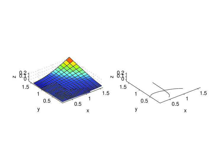
Figure 1: An example of a well-conditioned instance of SSI problem where collinear normal point methods and Koparkar’s algorithm require long computation time to solve.

Figure 2 shows a pair of collinear normal points in parametric space and the subdivision of domain at these points, as well as the intersection between the surfaces (Other pairs of collinear normal points are not shown). Parts of the intersection curves lie almost parallel to the boundaries of the created subdomains. In other words, the cuts made by the algorithm happen to intersect degenerately or nearly degenerately with the problem data. Thus, after the algorithm has made a subdivision of the domain based on the collinear normals, it must now recursively solve arbitrarily ill conditioned subproblems since the intersection point between the surface and the boundary curve is almost singular. The running time of algorithms for finding these intersection points typically depends on their conditioning (see, e.g., the RIA algorithm of [16]). Thus, the running time of the algorithm cannot be bounded in terms of the condition number of the input. Furthermore, ill-conditioning of the subproblems may cause unexpected inaccuracy of the solution of the original well-conditioned instance.

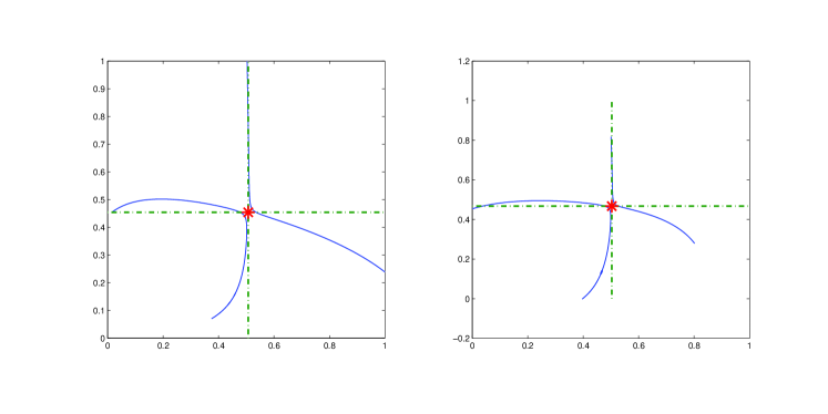
Figure 2: Intersection of the surfaces in Figure 1 in parametric space and splitting of the domains at a pair of collinear normal points showing that marching methods based on collinear normal points create ill-conditioned subproblem instances from a well-conditioned original instance. Solid lines are the intersections. Asterisks are the pair of collinear normal points. Dotted lines are the splitting lines at those points. To the left is the parametric domain of $p$. To the right is that of $q$.

4.2 Koparkar’s algorithm

Koparkar’s algorithm uses a test based on the contraction mapping theorem to determine if, in a given domain, a Newton-like method converges or the two surfaces do not intersect at all. If the Newton-like method is guaranteed to converge, the method is used to find part of the solution curves inside the domain. If the two surfaces are known not to intersect, the domain is discarded. Otherwise, each surface is subdivided by splitting their parametric domains into four, and the test is repeated on the created subdomains. This process continues until the entire domain is examined.

The test in Koparkar’s algorithm requires the ability to evaluate ranges of functions, which is typically accomplished by variety of interval arithmetics. None of these techniques can give the exact ranges, however; they yield supersets of the ranges. For this reason, the convergence test is likely to fail when part of the solution lies very close or directly on the border of a subcube in both $x_{1}x_{2}$-space and $x_{3}x_{4}$-space at the same time, which is not necessarily on or near the border of the original domain $[0,1]^{4}$. The same problem instance discussed in Section 4.1, which is shown in Figure 1, has such problem. The domain $[0,1]^{4}$ does not pass the test, and the domain is subdivided at the midpoints as shown in Figure 3. The subdomains now have solutions directly on a boundary. Koparkar’s algorithm needs to subdivide these subdomains to very small ones before the convergence test is satisfied. This example demonstrates that Koparkar’s algorithm is inefficient at solving certain well-conditioned instances. The algorithm may solve other instances with higher condition numbers but without any parts of the intersections near any boundaries of the subdivided subdomains faster than this well-conditioned instance.

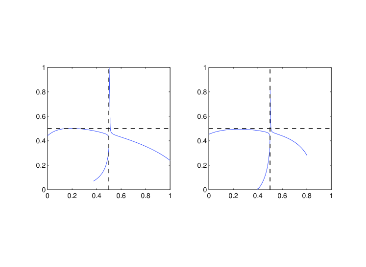
Figure 3: Intersection of the surfaces in Figure 1 in parametric space and subdomains created after the original domain $[0,1]^{4}$ fails Koparkar’s test. Due to part of the intersections lying on a boundary of a subdomain, Koparkar’s algorithm requires many subdivisions before those parts of the intersections can be located. Solid lines are the intersections. Dashed lines are the subdivision lines. To the left is the parametric domain of $p$. To the right is that of $q$.

5 The Kantorovich-Test Subdivision algorithm

This section describes our algorithm for the SDPS problem. Some details are postponed to the next section. Since we are interested in solutions of $f$ within the hypercube $[0,1]^{n+1}$, and the closed ball $\bar{B}(x,r)$ defined in the infinity norm is a hypercube, our algorithm uses the infinity norm for all of its norm computation. Therefore, for the rest of this article, the notation $\left\|\cdot\right\|$ is used to refer specifically to infinity norm.

During the computation, our algorithm maintains a list of explored regions defined as parts of the domain $[0,1]^{n+1}$ guaranteed by Kantorovich’s Theorem to contain only the solutions that have already been found. This list is used in addition to another test to determine whether to subdivide a hypercube. We define the Kantorovich test on a hypercube $X=\bar{B}(x^{0},r)$ as the application of Kantorovich’s Theorem on the point $x^{0}$ to the function $h^{(ik)}(x)=\left(f(x),x_{i}-k\right)^{T}$ for each $i=1,2,\ldots,n+1$ and any $k\in[x_{i}^{0}-r,x_{i}^{0}+r]$. The hypercube $[-.5,1.5]^{n+1}$ is used as the domain $D$ in the statement of the theorem, and $\left\|\left[\left(h^{(ik)}\right)^{\prime}(x^{0})\right]^{-1}h^{(ik)}(x^{0})\right\|$ is used as $\eta$. For $\omega$, we instead use $\hat{\omega}\geq\omega$, where $\hat{\omega}$ is defined by (13) below, as the minimal $\omega$ is too expensive to compute. The hypercube $X$ passes the Kantorovich test if there exists an $i\in\{1,2,\ldots,n+1\}$ such that for every $k\in[x_{i}^{0}-r,x_{i}^{0}+r]$, $\eta\hat{\omega}\leq 1/4$ and $\bar{B}(x^{0},\rho_{-})\subseteq D$.

The choice of $D$ mentioned in the previous paragraph is used in the analysis of the algorithm in Section 7, but in practice a smaller $D$ such that $B(x^{0},r)\subset D\subset[-.5,1.5]^{n+1}$ may be used. The advantage of using a smaller $D$ is that the Lipschitz constant $\hat{\omega}$ will be smaller, so the inequality $\eta\hat{\omega}\leq 1/4$ may be satisfied more easily (i.e., for larger hypercubes) than using the full $D$. The disadvantage, however, is that if $D$ is chosen too small, then the condition $B(x^{0},\rho^{-})\subset D$ of the theorem may be hard to satisfy. In particular, the choice $D=B(x^{0},r)$ would be unacceptable for this reason.

If $X$ passes the Kantorovich test, then three important consequences follow. First, $x^{0}$ is a fast starting point for $h^{(ik)}$ for the particular $i$ that satisfies the condition of the Kantorovich test and any $k\in[x_{i}^{0}-r,x_{i}^{0}+r]$. Second, the segment of the solution curve of $f$ that contains the root guaranteed by the conclusion of Kantorovich’s theorem is not a loop in $x_{1}x_{2}\cdots x_{n+1}$-space inside $X$ (although it may be part of a loop in the original domain). Third, an explored region for this segment of the solution curve can be derived. The explored region is

$$X_{E}=\left\{x:x_{i}^{0}-r\leq x_{i}\leq x_{i}^{0}+r\right\}\cap D\cap\bigcap_{k\in[x_{i}^{0}-r,x_{i}^{0}+r]}\left(\bar{B}(x^{0},\rho_{-}^{(k)})\cup B(x^{0},\rho_{+}^{(k)})\right),$$ (11)

where $\rho_{-}^{(k)}$ and $\rho_{+}^{(k)}$ are $\rho_{-}$ and $\rho_{+}$ in the statement of Kantorovich’s theorem with respect to $h^{(ik)}$. Observe that $X_{E}$ is a hyperrectangle in $\mathbb{R}^{n+1}$ and can be stored and computed succinctly as detailed in Section 6.2. Note also that the explored region provides an effective way to prevent the points on different but nearby solution curves from being incorrectly joined into the same curve.

The other test our algorithm uses is the exclusion test. For a given hypercube $X$, let $\hat{f}_{X}$ be the Bernstein polynomial that reparametrizes with $[0,1]^{n+1}$ the function defined by $f$ over $X$. In other words, $\hat{f}_{X}(q)\equiv f(\lambda(q))$, where $\lambda(q)$ is a composition of a dilation and translation (uniquely determined) such that $\lambda:[0,1]^{n+1}\rightarrow X$ is bijective. (See Section 6.3 for information how to efficiently compute $\hat{f}_{X}$.) The hypercube $X$ passes the exclusion test if the convex hull of the control points of $\hat{f}_{X}$ excludes the origin. It is a well-known property of the Bernstein-Bézier representation of a polynomial $f$ that $f(U)$ lies in the convex hull of its control points, where $U$ represents its natural parametric domain. Thus, if the hull of the coefficients of a polynomial system excludes the origin, this system has no solutions in the parametric domain. We can check whether the hull excludes the origin by solving a low-dimensional linear programming problem. Megiddo [15] showed that low-dimensional linear programming problems can be solved in linear time (i.e., linear in the number of control points), although we have not used Megiddo’s algorithm. Note that some other polynomial bases also have a similar exclusion test; refer to [20].

We now proceed to describe our algorithm, the Kantorovich-Test Subdivision algorithm or KTS in short.

Algorithm KTS:

• Let $Q$ be a queue with $[0,1]^{n+1}$ as its only entry. Set $S=\emptyset$.

• Repeat until $Q=\emptyset$

  1. Let $X$ be the hypercube at the front of $Q$. Remove $X$ from $Q$.

  2. If $X\not\subseteq X_{E^{\prime}}$ for all $X_{E^{\prime}}\in S$,

     • Perform the exclusion test on $X=\bar{B}(x^{0},r)$

     • If $X$ fails the exclusion test,

       1. Perform the Kantorovich test on $X$

       2. If $X$ passes the Kantorovich test,

          1. Perform Newton’s method on $h^{(ik)}$, where $i$ is the index that satisfies the condition of the Kantorovich test and $k=x_{i}^{0}-r$, starting from $x^{0}$ to find a zero $x^{*}$.

          2. Trace the segment of the solution curve using $x^{*}$ as the starting point and going toward $x_{i}^{0}+r$ direction until the $x_{i}=x_{i}^{0}+r$ boundary is reached.

          3. If the newly found segment is contained in any $X_{E^{\prime}}\in S$ (i.e. the segment has been found before), discard the segment.

          4. Otherwise, compute the new explored region $X_{E}$ according to (11). Set $S=S\cup\{X_{E}\}$.

       3. If either $X$ fails the Kantorovich test or $X$ passes the test with $X\not\subseteq X_{E}$, subdivide $X$ along all $n+1$ parametric axes into $2^{n+1}$ equal smaller hypercubes. Add these hypercubes to the end of $Q$.

• Check if any two segments of solution curves overlap. If so, remove the overlapping part from one of the segments.

• Join any two segments sharing an endpoint into one continuous curve. Repeat until there are no two curves sharing an endpoint.

A few remarks are needed regarding the description of the KTS algorithm.

• The subdivision in step 2.c is performed in the case that $X$ passes the Kantorovich test but $X\not\subseteq X_{E}$ because, in general, passing the Kantorovich test does not imply that there is only one solution curve in $X$.

• The check in step 2.b.iii is necessary since the segment detected by the Kantorovich test may be outside of $X$.

• For the same reason as above, certain parts of a solution curve may be traced twice and hence must be removed from one of the segments before the segments are joined. The overlapping segments can be detected by checking if an endpoint of a segment is inside an explored region of another segment. The segments sharing an endpoint can also be detected from explored regions in a similar manner. Note that there is no ambiguity in this step because an explored region, having passed the Kantorovich test, cannot contain more than one connected component of the solution.

• If the Kantorovich test is not applicable for a certain hypercube due to the Jacobian of the midpoint being singular, the hypercube is treated as if it fails the Kantorovich test and is then subdivided by step 2.c.

One property of KTS is that it is affinely invariant. In other words, left-multiplying $f$ with an $n\times n$ matrix $A$ prior to executing KTS does not change its behavior. This is the main reason that we introduced $\mathop{\rm{icond}}(f)$ earlier.

6 Implementation details

The implementations of certain steps of KTS are not apparent and thus are explained in detail in this section. While this section focuses only on the Bézier surface case, all the results herein can be generalized to certain other polynomial bases as mentioned in the introduction.

6.1 Computation of Lipschitz constant

For simplicity, denote $h^{(ik)}$ as $h$ when the choice of $(ik)$ is clear from context. The Lipschitz constant for $h^{\prime}(x^{0})^{-1}h^{\prime}\equiv g$, which is required for the Kantorovich test, is obtained from an upper bound over all $x\in[-.5,1.5]^{n+1}$ of the derivative of $g$

$$g^{\prime}(x)=\left(\frac{\partial^{2}\left(h^{\prime}(x^{0})^{-1}h\right)_{i}(x)}{\partial x_{j}\partial x_{k}}\right),$$

where $\left(h^{\prime}(x^{0})^{-1}h\right)_{i}(x)$ denotes the $i$th entry of $\left(h^{\prime}(x^{0})^{-1}h\right)(x)$. Let $\hat{g}$ be the Bernstein polynomial that reparametrizes with $[0,1]^{n+1}$ the surface defined by $g$ over $[-.5,1.5]^{n+1}$ (Refer to Section 6.3). We have

$$\max_{x\in[-.5,1.5]^{n+1}}\left\|g^{\prime}(x)\right\| = \frac{1}{2}\cdot\max_{x\in[0,1]^{n+1}}\left\|\hat{g}^{\prime}(x)\right\|$$

$$= \frac{1}{2}\cdot\max_{x\in[0,1]^{n+1}}\max_{\left\|y\right\|=1}\left\|\hat{g}^{\prime}(x)y\right\|$$

$$\leq \frac{1}{2}\cdot\max_{x\in[0,1]^{n+1}}\max_{i}\sum_{j=1}^{n+1}\sum_{k=1}^{n+1}|\hat{g}^{\prime}_{ijk}(x)|$$

$$\leq \frac{(n+1)^{2}}{2}\max_{i,j,k}\max_{x\in[0,1]^{n+1}}|\hat{g}^{\prime}_{ijk}(x)|.$$

Note that each entry of $\hat{g}^{\prime}$ can be written as a Bernstein polynomial efficiently because

$$\frac{dZ_{i,m}(t)}{dt}=m\left(Z_{i-1,m-1}(t)-Z_{i,m-1}(t)\right),$$ (12)

where $Z_{-1,m-1}(t)=Z_{m,m-1}(t)=0$, which can be used to compute the control points of the derivatives in Bernstein basis from a given Bernstein polynomial directly. Hence, the maximum absolute value of the control points of $\hat{g}^{\prime}_{ijk}$ when written in Bernstein basis is an upper bound of $\max_{x\in[0,1]^{n+1}}|\hat{g}^{\prime}_{ijk}(x)|$. Let $\hat{\omega}$ denote the Lipschitz constant computed in this manner, that is,

$$\hat{\omega}\equiv\frac{(n+1)^{2}}{2}\max_{i,j,k,i_{1},i_{2},\ldots,i_{n+1}}\|\hat{g}^{\prime}_{ijk,i_{1},i_{2},\ldots,i_{n+1}}\|,$$ (13)

$\hat{g}^{\prime}_{ijk,i_{1},i_{2},\ldots,i_{n+1}}$ are the control points of $\hat{g}^{\prime}_{ijk}$.

6.2 The Kantorovich test and solution curve tracing

Recall that for a hypercube $X$ to pass the Kantorovich test, there must exist an $i\in\{1,2,\ldots,n+1\}$ satisfying $\eta\hat{\omega}\leq 1/4$ and $\bar{B}(x^{0},\rho_{-})\subseteq D$ for all functions $h^{(ik)}$’s where $k\in[x^{0}_{i}-r,x^{0}_{i}+r]$. The algorithm, however, need not explicitly check the conditions for all values of $k$. Notice that $\hat{\omega}$ and $D$ are independent of $k$ and $\rho_{-}$ is an increasing function of $\eta$. For these reasons, KTS only needs to check the conditions for the value of $k$ that maximizes $\eta$. Similarly, the explored region $X_{E}$ can be computed solely from the maximizer $k$. But note also that $\eta$ is linear in $k$, which means that the value of $k$ maximizing $\eta$ is either $x^{0}_{i}-r$ or $x^{0}_{i}+r$.

After a hypercube passes the Kantorovich test, the segment of the solution curve detected by the test must be traced. Since the Kantorovich test guarantees that performing Newton’s method on $h^{(ik)}$ starting on $x^{0}$ converges for any $k\in[x^{0}_{i}-r,x^{0}_{i}+r]$, we can trace the segment by repeating Newton’s method starting on $x^{0}$ for many different values of $k$ to locate the points on the segment of the solution curve. Alternatively, we can perform Newton’s method on $h^{(i,x^{0}_{i}-r)}$ starting on $x^{0}$ to find a point $x^{1}$ on the segment, use $x^{1}$ as the starting point for Newton’s method on $h^{(i,x^{0}_{i}-r+\epsilon)}$, $\epsilon>0$, to find the next point $x^{2}$ on the segment, use $x^{2}$ as the starting point on $h^{(i,x^{0}_{i}-r+2\epsilon)}$ to find the next point on the segment, and so on.

6.3 Reparametrization

There are two steps of KTS involving reparametrization of polynomials in Bernstein basis, namely the exclusion test and the computation of the Lipschitz constant for the Kantorovich test. “Reparametrization” in this context means the computation of new control points that describe the same function with respect to the new parameter domain. Both steps require the reparametrization with $[0,1]^{n+1}$ of Bernstein polynomials with $n+1$ variables, which is a straightforward extension of reparametrization with $[0,1]^{2}$ of bivariate Bernstein polynomials. An example of efficient algorithms for reparametrizing bivariate Bernstein polynomials with $[0,1]^{2}$ is discussed in [20]. Alternatively, the polynomials can be reparametrized by two applications of the de Casteljau algorithm [16]; one to reparametrize the right endpoints with $1$ and another to reparametrize the left endpoints with $0$.

7 Time complexity analysis

In this section, we prove a number of theorems leading to the theorem regarding the running time of the KTS algorithm. Since both the exclusion test and the computation of the Lipschitz constant in the Kantorovich test use the control points in their computations, it is useful to find the relationship between the control points and the function values of the polynomial defined by them. Recall that $M$ is defined as the maximum norm among control points of $f$ and was denoted $\|f\|$ earlier.

We have already shown that $f(x)$ and $f^{\prime}(x)$ are bounded by $M$ in $(\ref{eq:fMbound})$ and $(\ref{eq:fpMbound})$. Using the same logic, we can derive a Lipschitz bound on $f^{\prime}(x)$, i.e., an upper bound on $f^{\prime\prime}$, as follows:

$$\|f^{\prime}(x)-f^{\prime}(y)\|\leq 4(n+1)\max(m_{1},\ldots,m_{n+1})^{2}M\|x-y\|.$$ (14)

The use of the Kantorovich theorem requires a Lipschitz bound for a slightly larger region. If we require a Lipschitz bound for $f^{\prime}(x)$ over $[-\epsilon,1+\epsilon]^{n+1}$, then we can argue based on the deCasteljau algorithm for evaluating Bézier polynomials that

$$\|f^{\prime}(x)-f^{\prime}(y)\|\leq 4(n+1)(1+\epsilon)^{\max(m_{1},\ldots,m_{n+1})}\max(m_{1},\ldots,m_{n+1})^{2}M\|x-y\|.$$ (15)

Another useful inequality is that for any $x\in[0,1]^{n+1}$,

$$M\|f^{\prime}(x)^{\dagger}\|\geq 1/\left(2(n+1)\max(m_{1},\ldots,m_{n+1})\right).$$ (16)

Equation $(\ref{eq:Mpinvineq})$ can be established by multiplying both sides of $(\ref{eq:fpMbound})$ by $\|f^{\prime}(x)^{\dagger}\|$ and then using the fact that $\|f^{\prime}(x)\|\cdot\|f^{\prime}(x)^{\dagger}\|\geq\|f^{\prime}(x)f^{\prime}(x)^{\dagger}\|=\|I\|=1$ for any matrix $p$-norm, and for the infinity-norm in particular.

Now, we establish a bound that reverses $(\ref{eq:fMbound})$, namely,

$$M\leq\theta\max_{0\leq x_{1},x_{2},\ldots,x_{n+1}\leq 1}\left\|f(x)\right\|$$ (17)

for any polynomial $f$, where $\theta$ is as defined as follows.

$$\theta=\theta(m_{1},\ldots,m_{n+1}) = \prod_{k=1}^{n+1}\left(\sum_{i=0}^{m_{k}}\prod_{i^{\prime}\neq i}\frac{\max\{|m_{k}-i^{\prime}|,|i^{\prime}|\}}{|i-i^{\prime}|}\right)$$

$$= O\left(m_{1}^{m_{1}+1}m_{2}^{m_{2}+1}\cdots m_{n+1}^{m_{n+1}+1}\right).$$

This value of $\theta$ is specific to the choice of the Bernstein-Bézier basis; see [20] for a discussion of other bases.

Our proof of $(\ref{theta_eq})$ is based on establishing a similar result for univariate polynomials as shown by the following lemmas.

Theorem 7.1 (Srijuntongsiri and Vavasis [20]).

Let $f(t)$ be a polynomial system

$$\begin{array}[]{llll}f(t)&=&\sum_{i=0}^{m}b_{i}Z_{i,m}(t),&0\leq t\leq 1,\end{array}$$

where $b_{i}\in\mathbb{R}^{d}$. The norm of the coefficients can be bounded by

$$\left\|b_{i}\right\|\leq\xi_{B}(m)\max_{t:0\leq t\leq 1}\left\|f(t)\right\|,$$

where

$$\xi_{B}(m)=\sum_{i=0}^{m}\prod_{j=0,1,\ldots,i-1,i+1,\ldots,m}\frac{\max\{|m-j|,|j|\}}{|i-j|}=O(m^{m+1}).$$

Lemma 7.2.

Let $l$ and $h$ be constants satisfying $l<h$. Let $n$ be a given positive integer. Suppose there exists a function $\xi(m)$ satisfying

$$\left\|a_{i}\right\|\leq\xi(m)\max_{l\leq t\leq h}\left\|g(t)\right\|$$ (18)

for any $a_{i}\in\mathbb{R}^{d}$ $(i=0,1,\ldots,m)$ and any univariate polynomial $g(t)=\sum_{i=0}^{m}a_{i}\phi_{i}(t)$, where $\phi_{i}(t)$ denotes the polynomial basis. Suppose also there exists a function $\zeta(m_{1},m_{2},\ldots,m_{n})$ satisfying

$$\left\|\bar{a}_{i_{1},i_{2},\ldots,i_{n}}\right\|\leq\zeta(m_{1},m_{2},\ldots,m_{n})\max_{l\leq x_{1},x_{2},\ldots,x_{n}\leq h}\left\|\bar{g}(x_{1},x_{2},\ldots,x_{n})\right\|$$ (19)

for any $\bar{a}_{i_{1},i_{2},\ldots,i_{n}}\in\mathbb{R}^{d}$ $(i_{j}=0,1,\ldots,m_{j})$ and any polynomial in $n$ variables

$$\bar{g}(x_{1},x_{1},\ldots,x_{n})=\sum_{i_{1}=0}^{m_{1}}\sum_{i_{2}=0}^{m_{2}}\cdots\sum_{i_{n}=0}^{m_{n}}\bar{a}_{i_{1},i_{2},\ldots,i_{n}}\phi_{i_{1}}(x_{1})\phi_{i_{2}}(x_{2})\cdots\phi_{i_{n}}(x_{n}).$$

Then

$$\left\|b_{i_{1},\ldots,i_{n+1}}\right\|\leq\zeta(m_{1},m_{2},\ldots,m_{n})\xi(m_{n+1})\max_{l\leq x_{1},x_{2},\ldots,x_{n+1}\leq h}\left\|f(x_{1},x_{2},\ldots,x_{n+1})\right\|$$ (20)

for any $b_{i_{1},\ldots,i_{n+1}}\in\mathbb{R}^{d}$ $(i_{j}=0,1,\ldots,m_{j})$, where $f$ is the polynomial in $n+1$ variables defined by

$$f(x_{1},x_{2},\ldots,x_{n+1})=\sum_{i_{1}=0}^{m_{1}}\cdots\sum_{i_{n+1}=0}^{m_{n+1}}b_{i_{1},\cdots,i_{n+1}}\phi_{i_{1}}(x_{1})\cdots\phi_{i_{n+1}}(x_{n+1}).$$ (21)

Proof.

Let $f(x_{1},x_{2},\ldots,x_{n+1})$ be an arbitrary polynomial defined as in (21). For any $n$-tuple $I^{\prime}=(i^{\prime}_{1},i^{\prime}_{2},\ldots,i^{\prime}_{n})$ $(i^{\prime}_{j}=0,1,\ldots,m_{j})$, define

$$g_{I^{\prime}}(x_{n+1})=\sum_{i_{n+1}=0}^{m_{n+1}}b_{i^{\prime}_{1},i^{\prime}_{2},\ldots,i^{\prime}_{n},i_{n+1}}\phi_{i_{n+1}}(x_{n+1}).$$

Applying (18) to $g_{I^{\prime}}$ yields

$$\left\|b_{i^{\prime}_{1},i^{\prime}_{2},\ldots,i^{\prime}_{n},i_{n+1}}\right\|\leq\xi(m_{n+1})\max_{l\leq x_{n+1}\leq h}\left\|g_{I^{\prime}}(x_{n+1})\right\|$$ (22)

for any $b_{i^{\prime}_{1},i^{\prime}_{2},\ldots,i^{\prime}_{n},i_{n+1}}$ $(i_{n+1}=0,1,\ldots,m_{n+1})$. Let $x^{*}_{I^{\prime}}$ be a point where $\max_{l\leq x_{n+1}\leq h}\left\|g_{I^{\prime}}(x_{n+1})\right\|$ is achieved. Define

$$k_{I^{\prime}}(x_{1},x_{2},\ldots,x_{n})=\sum_{i_{1}=0}^{m_{1}}\sum_{i_{2}=0}^{m_{2}}\cdots\sum_{i_{n}=0}^{m_{n}}\sum_{i_{n+1}=0}^{m_{n+1}}b_{i_{1},i_{2},\ldots,i_{n+1}}\phi_{i_{1}}(x_{1})\phi_{i_{2}}(x_{2})\cdots\phi_{i_{n}}(x_{n})\phi_{i_{n+1}}(x^{*}_{I^{\prime}}).$$

Applying (19) to $k_{I^{\prime}}$ yields

$$\left\|\sum_{i_{n+1}=0}^{m_{n+1}}b_{i_{1},\ldots,i_{n+1}}\phi_{i_{n+1}}(x^{*}_{I^{\prime}})\right\|\leq\zeta(m_{1},m_{2},\ldots,m_{n})\max_{l\leq x_{1},\ldots,x_{n}\leq h}\left\|k_{I^{\prime}}(x_{1},\ldots,x_{n})\right\|$$ (23)

for any $(i_{1},i_{2},\ldots,i_{n})$ ($i_{j}=0,1,\ldots,m_{j}$). Consequently, by combining (22) and (23),

$$\left\|b_{i^{\prime}_{1},i^{\prime}_{2},\ldots,i^{\prime}_{n},i_{n+1}}\right\| \leq \xi(m_{n+1})\left\|g_{I^{\prime}}(x^{*}_{I^{\prime}})\right\|$$

$$= \xi(m_{n+1})\left\|\sum_{i_{n+1}=0}^{m_{n+1}}b_{i_{1},\ldots,i_{n+1}}\phi_{i_{n+1}}(x^{*}_{I^{\prime}})\right\|$$

$$\leq \xi(m_{n+1})\zeta(m_{1},m_{2},\ldots,m_{n})\max_{l\leq x_{1},\ldots,x_{n}\leq h}\left\|k_{I^{\prime}}(x_{1},\ldots,x_{n})\right\|$$

$$\leq \xi(m_{n+1})\zeta(m_{1},m_{2},\ldots,m_{n})\max_{l\leq x_{1},x_{2},\ldots,x_{n+1}\leq h}\left\|f(x_{1},x_{2},\ldots,x_{n+1})\right\|.$$

∎

Hence, (17) holds by induction using Theorem 7.1 as the basis and Lemma 7.2 as the inductive step.

Recall that the Lipschitz constant $\hat{\omega}$ given by (13) is not the smallest Lipschitz constant for $h^{\prime}(x^{0})^{-1}h$ over $D=[-.5,1.5]^{n+1}$. However, we can show that $\hat{\omega}\leq\left((n+1)^{2}/2\right)\theta\omega$, where $\omega$ denotes the smallest Lipschitz constant for $h^{\prime}(x^{0})^{-1}h$ over $D$. Since $\hat{\omega}$ is computed from the absolute values of the control points of $\hat{g}^{\prime}_{ijk}(x)$, by (17),

$$\hat{\omega} \leq \frac{(n+1)^{2}}{2}\theta\max_{i,j,k}\max_{x\in[0,1]^{n+1}}\left|\hat{g}^{\prime}_{ijk}(x)\right|$$ (24)

$$= \frac{(n+1)^{2}}{2}\theta\max_{i,j,k}\max_{x\in D}\left|g^{\prime}_{ijk}(x)\right|$$

$$\leq \frac{(n+1)^{2}}{2}\theta\max_{x\in D}\left\|g^{\prime}(x)\right\|=\frac{(n+1)^{2}}{2}\theta\omega.$$

With this bound on $\hat{\omega}$, we can now analyze the behavior of the Kantorovich test.

The following is the main technical result of this article.

Theorem 7.3.

Let $f(x)=f(x_{1},x_{2},\ldots,x_{n+1})$ be a Bernstein polynomial system in $n$ dimensions such that $\mathop{\rm{cond}}(f)<\infty$. Let $x^{0}$ be a point in $[0,1]^{n+1}$. Let $r>0$ be such that $\bar{B}(x^{0},r)\subseteq[0,1]^{n+1}$. If

$$r<\left(\frac{c_{0}}{\mathop{\rm{cond}}(f)}\right)^{2},$$ (25)

where

$$c_{0}=\frac{1}{64(n+1)^{3}\theta\cdot 1.5^{\max(m_{1},m_{2},\ldots,m_{n+1})}\max(m_{1},m_{2},\ldots,m_{n+1})^{2}},$$ (26)

then either

1. The hypercube $\bar{B}(x^{0},r)$ passes the Kantorovich test and the associated explored region $X_{E}$ contains $X$, or

2. The hypercube $\bar{B}(x^{0},r)$ passes the exclusion test.

Proof.

Let $X$ denote the hypercube $\bar{B}(x^{0},r)$. Let us introduce additional notation for frequently used quantities. Let $\phi$ stand for $\|f(x^{0})\|$, and let $\pi$ stand for $\|f^{\prime}(x^{0})^{\dagger}\|$. The proof is divided into two cases by the relative value of the two terms in the definition of condition number $(\ref{cond_def})$ evaluated at $x^{0}$. Let

$$c_{1}=\sqrt{64(n+1)^{3}\theta\cdot(1.5)^{\max(m_{1},m_{2},\ldots,m_{n+1})}\max(m_{1},m_{2},\ldots,m_{n+1})^{2}}.$$ (27)

Case 1: $c_{1}M\pi\leq\sqrt{M/\phi}$.

Note that this case encompasses the possibility that $\phi=0$, i.e., that $x^{0}$ lies on a solution curve. On the other hand, this case requires $\pi<\infty$, i.e., $\mathop{\rm{rank}}(()f^{\prime}(x^{0}))=n$. Note that $M\pi$ is the second term of $(\ref{cond_def})$ evaluated at $x^{0}$ while $\sqrt{M/\phi}$ is the first term. Therefore, $\mathop{\rm{cond}}(f)\geq\min(M\pi,M/\phi)\geq\min(M\pi,c_{1}^{2}M^{2}\pi^{2}).$ Since $c_{1}M\pi\geq 1$ and $c_{1}^{2}M\pi\geq 1$ (combine $(\ref{eq:Mpinvineq})$ and $(\ref{eq:k1def})$), it follows that the second term dominates the first, hence

$$\mathop{\rm{cond}}(f)\geq M\pi.$$ (28)

By the hypothesis for this case, $c_{1}^{2}M^{2}\pi^{2}\leq M/\phi$, i.e.,

$$\phi\leq 1/(c_{1}^{2}M\pi^{2}).$$ (29)

Let $v(x^{0})$ be the unit-length null vector of $f^{\prime}(x^{0})$, i.e., $f^{\prime}(x^{0})v(x^{0})=0$, $\left\|v(x^{0})\right\|=1$. Let $i$ be such that $|v_{i}(x^{0})|=1$. Define

$$h(x)=\left(\begin{array}[]{cc}f(x)\\ x_{i}-k\end{array}\right)$$

for an arbitrary $k\in[x^{0}_{i}-r,x^{0}_{i}+r]$. By using the facts that $\left\|v(x^{0})\right\|=1$, $|v_{i}(x^{0})|=1$, and

$$h^{\prime}(x^{0})^{-1}=\left(\begin{array}[]{c}f^{\prime}(x^{0})\\ e_{i}^{T}\end{array}\right)^{-1}=\left(\left(I-\frac{v(x^{0})e_{i}^{T}}{v(x^{0})^{T}e_{i}}\right)f^{\prime}(x^{0})^{\dagger},\frac{v(x^{0})}{v(x^{0})^{T}e_{i}}\right),$$

where $e_{i}$ denotes the $i$th column of the identity matrix, it is seen that

$$\eta\equiv\left\|h^{\prime}(x^{0})^{-1}h(x^{0})\right\|\leq 2\left(\left\|f^{\prime}(x^{0})^{\dagger}f(x^{0})\right\|+r\right),$$ (30)

for any $k\in[x^{0}_{i}-r,x^{0}_{i}+r]$. (Note that in the infinity norm, $\|I-ve_{i}^{T}/(v^{T}e_{i})\|\leq 2$, where $i$ is the index such that $\|v\|=|v^{T}e_{i}|$.) The first parenthesized term on the right-hand side of $(\ref{eta_ineq})$ is clearly bounded by $\pi\phi$, which in turn is bounded by $1/(c_{1}^{2}M\pi)$ by $(\ref{eq:case1phibd})$.

It follows from $(\ref{eq:case1condf})$, $(\ref{eq:Mpinvineq})$, and $(\ref{eq:k0def})$ that $c_{0}/\mathop{\rm{cond}}(f)\leq 1$, hence $(c_{0}/\mathop{\rm{cond}}(f))^{2}\leq(c_{0}/\mathop{\rm{cond}}(f))$. Combining this with $(\ref{deltahatcond})$ and $(\ref{eq:case1condf})$ yields

$$r\leq c_{0}/\mathop{\rm{cond}}(f)\leq c_{0}/(M\pi).$$ (31)

Thus, proceeding from $(\ref{eta_ineq})$,

$$\eta\leq\frac{2(c_{0}+1/c_{1}^{2})}{M\pi}.$$ (32)

Note that $4(n+1)(1.5)^{\max(m_{1},\ldots,m_{n+1})}\max(m_{1},\ldots,m_{n+1})^{2}M$ is a Lipschitz constant of $f^{\prime}$ on $[-5,1.5]^{n+1}$ by $(\ref{eq:exLip})$. Consequently, $4(n+1)(1.5)^{\max(m_{1},\ldots,m_{n+1})}\cdot\linebreak\max(m_{1},\ldots,m_{n+1})^{2}M\pi$ is a Lipschitz constant of $f^{\prime}(x^{0})^{\dagger}f^{\prime}$ on $[-5,1.5]^{n+1}$. From this bound, we derive a Lipschitz constant $\omega$ for $h^{\prime}(x^{0})^{-1}h^{\prime}$ over $[-.5,1.5]^{n+1}$ as follows.

$$\omega = \max_{y,z\in D;y\neq z}\frac{\left\|h^{\prime}(x^{0})^{-1}\left(h^{\prime}(y)-h^{\prime}(z)\right)\right\|}{\left\|y-z\right\|}$$

$$= \max_{y,z\in D;y\neq z}\frac{1}{\left\|y-z\right\|}\cdot\left\|\left(I-\frac{v(x^{0})e_{i}^{T}}{v(x^{0})^{T}e_{i}}\right)f^{\prime}(x^{0})^{\dagger}\left(f^{\prime}(y)-f^{\prime}(z)\right)\right\|$$

$$\leq \max_{y,z\in D;y\neq z}\frac{2\left\|f^{\prime}(x^{0})^{\dagger}\left(f^{\prime}(y)-f^{\prime}(z)\right)\right\|}{\left\|y-z\right\|}$$

$$\leq 2\pi\cdot\max_{y,z\in D;y\neq z}\frac{\|f^{\prime}(y)-f^{\prime}(z)\|}{\left\|y-z\right\|}$$

$$\leq 8(n+1)(1.5)^{\max(m_{1},\ldots,m_{n+1})}\max(m_{1},\ldots,m_{n+1})^{2}M\pi.$$

For the last line, we used $(\ref{eq:exLip})$. But from $(\ref{hodef})$,

$$\hat{\omega}\leq\frac{(n+1)^{2}}{2}\theta\omega\leq 4(n+1)^{3}\theta(1.5)^{\max(m_{1},\ldots,m_{n+1})}\max(m_{1},\ldots,m_{n+1})^{2}M\pi$$ (33)

where $\omega$ is the Lipschitz constant for $h^{\prime}(x^{0})^{-1}h^{\prime}$ over $[-.5,1.5]^{n+1}$ and $\hat{\omega}$ is the computed Lipschitz constant for $h^{\prime}(x^{0})^{-1}h^{\prime}$ over $D$ as defined in (13).

Combining $(\ref{eq:etabound})$ with $(\ref{eq:omegahat})$ yields

$$\eta\hat{\omega}<8(n+1)^{3}\theta(1.5)^{\max(m_{1},\ldots,m_{n+1})}\max(m_{1},\ldots,m_{n+1})^{2}(c_{0}+1/c_{1}^{2}).$$ (34)

By choice of $c_{0}$ and $c_{1}$ in $(\ref{eq:k0def})$ and $(\ref{eq:k1def})$ respectively, we see that $\eta\hat{\omega}<1/4$ for any $k\in[x^{0}_{i}-r,x^{0}_{i}+r]$, which is one of the conditions for $X$ to pass the Kantorovich test.

For the other condition, note that $\sqrt{1-2h}\geq 1-2h$ for $0\leq h\leq 1/2$. Therefore,

$$\rho_{-} = \frac{1-\sqrt{1-2\eta\hat{\omega}}}{\hat{\omega}}$$ (35)

$$\leq 2\eta$$

$$\leq \frac{4(c_{0}+1/c_{1}^{2})}{M\pi}\qquad\mbox{(by $(\ref{eq:etabound})$)}$$

$$\leq 8(n+1)(c_{0}+1/c_{1}^{2})\max(m_{1},\ldots,m_{n+1})\qquad\mbox{(by $(\ref{eq:Mpinvineq})$)}.$$

By choice of $c_{0}$ and $c_{1}$, we conclude that $\rho_{-}<1/2$ and therefore $X\subset[-.5,1.5]^{n+1}$, the domain for which $\omega$ is a Lipschitz constant. This proves that $X$ satisfies the Kantorovich conditions.

Finally, the associated explored region $X_{E}$ contains $X$ because

$$\rho_{+} = \frac{1+\sqrt{1-2\eta\hat{\omega}}}{\hat{\omega}}$$

$$\geq \frac{1}{\hat{\omega}}$$

$$\geq \frac{1}{4(n+1)^{3}\theta(1.5)^{\max(m_{1},\ldots,m_{n+1})}\max(m_{1},\ldots,m_{n+1})^{2}M\pi}\qquad\mbox{(by $(\ref{eq:omegahat})$)}$$

$$\geq r,$$

for any $k\in[x^{0}_{i}-r,x^{0}_{i}+r]$. The last line follows from $(\ref{eq:k0def})$ and $(\ref{eq:rbdcase1})$.

Case 2: $c_{1}M\pi\geq\sqrt{M/\phi}$.

Note that this case encompasses the possibility that $\pi=\infty$, i.e., $\mathop{\rm{rank}}(()f^{\prime}(x^{0}))<n$. On the other hand, this case requires $\phi>0$, i.e., $x^{0}$ is not a root. Since $\mathop{\rm{cond}}(f)\geq\min(M\pi,M/\phi)\geq\min(\sqrt{M/\phi}/c_{1},M/\phi)$, we conclude

$$\mathop{\rm{cond}}(f)\geq\sqrt{\frac{M}{c_{1}^{2}\phi}},$$ (36)

which implies by $(\ref{deltahatcond})$ that

$$r\leq\frac{c_{0}^{2}c_{1}^{2}\phi}{M}.$$ (37)

Select an arbitrary $x\in B(x^{0},r)$. We now derive a bound on $f(x)-f(x^{0})$ by applying the fundamental theorem of calculus.

$$\|f(x)-f(x^{0})\| = \left\|\int_{0}^{1}f^{\prime}(x^{0}+t(x-x^{0}))(x-x^{0})\,dt\right\|$$

$$\leq \int_{0}^{1}\|f^{\prime}(x^{0}+t(x-x^{0}))\|\,dt\cdot\|x-x^{0}\|$$

$$\leq r\int_{0}^{1}2(n+1)\max(m_{1},\ldots,m_{n+1})M\,dt\qquad\mbox{(by $(\ref{eq:fpMbound})$)}$$

$$= 2r(n+1)\max(m_{1},\ldots,m_{n+1})M$$

$$\leq 2(n+1)c_{0}^{2}c_{1}^{2}\max(m_{1},\ldots,m_{n+1})\phi\qquad\mbox{(by $(\ref{eq:case2rbd})$)}$$

$$\leq \frac{\phi}{2\theta}\qquad\mbox{(by $(\ref{eq:k0def})$ and $(\ref{eq:k1def})$).}$$

Thus, by definition of $\phi$,

$$\theta\cdot\left\|f(x)-f(x^{0})\right\|<\left\|f(x^{0})\right\|.$$ (38)

Define $\hat{f}(\hat{x})$ such that

$$\hat{f}(\hat{x}_{1},\hat{x}_{2},\ldots,\hat{x}_{n+1}) = f(2r\hat{x}_{1}+x^{0}_{1}-r,2r\hat{x}_{2}+x^{0}_{2}-r,\ldots$$ (39)

$$\hskip 11.0pt2r\hat{x}_{n+1}+x^{0}_{n+1}-r).$$

In other word, $\hat{f}$ is a polynomial that reparametrizes with $[0,1]^{n+1}$ the surface defined by $f$ over $X$. In terms of $\hat{f}$, (38) is equivalent to

$$\theta\cdot\left\|\hat{f}(\hat{x})-\hat{f}(\hat{x}^{0})\right\|<\left\|\hat{f}(\hat{x}^{0})\right\|$$

for an arbitrary $\hat{x}\in[0,1]^{n+1}$, where $\hat{x}$ is the rescaled $x$, and $\hat{x}^{0}$ is the rescaled $x^{0}$ according to (39). In particular,

$$\theta\cdot\max_{\hat{x}\in[0,1]^{n+1}}\left\|\hat{f}(\hat{x})-\hat{f}(\hat{x}^{0})\right\|<\left\|\hat{f}(\hat{x}^{0})\right\|.$$ (40)

Let $g(\hat{x})\equiv\hat{f}(\hat{x})-\hat{f}(\hat{x}^{0})$. By (17),

$$\left\|c_{i_{1},\ldots,i_{n+1}}\right\|\leq\theta\cdot\max_{\hat{x}\in[0,1]^{n+1}}\left\|g(\hat{x})\right\|,$$ (41)

for any control point $c_{i_{1},\ldots,i_{n+1}}$ of $g(\hat{x})$, which is equivalent to

$$\left\|a_{i_{1},\ldots,i_{n+1}}-\hat{f}(\hat{x}^{0})\right\|\leq\theta\cdot\max_{\hat{x}\in[0,1]^{n+1}}\left\|\hat{f}(\hat{x})-\hat{f}(\hat{x}^{0}))\right\|,$$ (42)

for any control point $a_{i_{1},\ldots,i_{n+1}}$ of $\hat{f}(\hat{x})$ (since a constant additive term to a polynomial corresponds to a translation of all of its control points). Substituting (42) into the left-hand side of (40) yields

$$\left\|a_{i_{1},\ldots,i_{n+1}}-\hat{f}(\hat{x}^{0})\right\|<\left\|\hat{f}(\hat{x}^{0})\right\|,$$ (43)

which implies that the convex hull of the control points of $\hat{f}(\hat{x})$ does not contain the origin. Therefore, $X$ passes the exclusion test. ∎

8 Computational results

The KTS algorithm is implemented in Matlab and is tested against a number of problem instances with three equations and four variables of varying condition numbers. Higher dimension problems, especially the ill-conditioned instances, require too much computation time due to the large number of hypercubes that must be considered. We estimate the condition number by evaluating $\min\left\{1/\left\|f(x^{0})\right\|,\left\|f^{\prime}(x^{0})^{\dagger}\right\|\right\}$ at the center point $x^{0}$ of every square considered by KTS during its execution and also at uniformly sampled points in $[0,1]^{4}$.

Table 3 compares the efficiency of KTS for each test problem with its condition number. The total number of hypercubes examined by KTS during the entire computation, the width of the smallest hypercube among those examined, and the maximum number of Newton iterations to converge are reported. Note that the high number of Newton iterations of some test cases (the $9$th and $10$th rows of Table 3) is because the Jacobians of the zeros are ill-conditioned causing large roundoff error in the computation of the Newton iterations.

$\max\{m_{1},m_{2},m_{3},m_{4}\}$	$\mathop{\rm{cond}}(f)$	Number of	Smallest	Max. Newton
		hypercubes	width	iterations
2	6.60	641	.03125	3
2	11.5	3089	.01563	3
2	15.5	673	.03125	3
3	24.0	145	.06250	-
3	50.0	4273	.00781	3
3	120	1009	.00391	3
3	$2.40\times 10^{3}$	18177	.00049	3
3	$9.88\times 10^{4}$	15841	.00195	4
3	$1.86\times 10^{7}$	28881	.00098	7
3	$2.66\times 10^{7}$	29649	.00098	7

Table 3: Efficiency of KTS algorithm on problems of different condition numbers.

9 Conclusion and future directions

We present the KTS algorithm for solving systems of polynomial equations with one more unknowns than the number of polynomials. By using the combination of subdivision and Kantorovich’s theorem, our algorithm can take advantage of the quadratic convergence of Newton’s method without the problems of divergence and missing some solutions that commonly occur with Newton’s method. We also show that the efficiency of KTS has an upper bound that depends solely on the condition number of the problem instance. Nevertheless, there are a number of questions left unanswered by this article such as

• Tighter bound on $r$. Some of the bounds in Section 7 appear loose and could potentially underestimate the performance of the algorithm. For example, the scalars may be loose, and one step in the argument preceding $(\ref{eq:rbdcase1})$ uses the weak bound that $x^{2}\geq x$ since $x\geq 1$. Thus, it seems like there is room for tightening the analysis.

  A second limitation of our analysis is that we establish a lower bound on the smallest hypercube size, which indirectly places an upper bound on the total number of hypercubes explored by the KTS algorithm (and hence its running time). This upper bound, however, is usually far from tight as illustrated by our computational experiments. Thus, a different analysis that addresses the number of hypercubes more directly would be useful.

• Using KTS in floating point arithmetic. In the presence of roundoff error, we may need to make adjustments for KTS to be able to guarantee that the computed intersections are accurate and that all of the solutions are found.

• Handling singular solutions and degenerate instances. Instances containing singular solutions or degeneracy are ill-posed, and our proposed KTS algorithm does not aim at handling such instances. Certain applications, however, look for singular solutions or solutions to degenerate instances. Further investigation on extending KTS to handle these situations would be beneficial.

• Other representations of $f$. As mentioned in the introduction, we assume that $f$ is specified by its $(m_{1}+1)(m_{2}+1)\cdots(m_{n+1}+1)$ Bernstein-Bézier control points. In many applications, however, there may be a more parsimonious representation. For example, in the SSI problem, two surfaces of bi-degree $(m_{1},m_{2})$ are separately each represented by $(m_{1}+1)(m_{2}+1)$ control points, hence $f=p_{1}-p_{2}$ is fully described by $2(m_{1}+1)(m_{2}+1)$ control points rather than the $(m_{1}+1)^{2}(m_{2}+1)^{2}$ control points needed for the general case. It would be useful if the KTS algorithm could work directly on a more concise representation.

• Extension to general underdetermined polynomial systems. Polynomial systems with $n$ equations and $m>n+1$ unknowns generally contain higher dimension solutions. The subdivision and exclusion test ideas still hold for the general case, but a different technique is needed to trace an approximation to the intersection surface.

10 Acknowledgements

We benefited from a helpful discussion with F. Cucker about condition numbers.

References

- [1] P. Bürgisser, F. Cucker, and M. Lotz. The probability that a slightly perturbed numerical analysis problem is difficult. Math. Comp., 77:1559–1583, 2008.
- [2] F. Chaitin-Chatelin and V. Frayssé. Lectures on finite precision computations. SIAM, 1996.
- [3] F. Cucker, T. Krick, G. Malajovich, and M. Wschebor. A numerical algorithm for zero counting. II: Distance to ill-posedness and smoothed analysis. To appear, J. Fixed Point Theory Appl, 2009.
- [4] J. Demmel. The probability that a numerical analysis problem is difficult. Math. Comp., 50:449–480, 1988.
- [5] P. Deuflhard and G. Heindl. Affine invariant convergence theorems for Newton’s method and extensions to related methods. SIAM J. Numer. Anal., 16:1–10, 1980.
- [6] G. Farin. Curves and Surfaces for CAGD: A Practical Guide. Academic Press, 5 edition, 2002.
- [7] R. T. Farouki and T. N. T. Goodman. On the optimal stability of the bernstein basis. Mathematics of Computation, 65(216):1553– 1566, October 1996.
- [8] R. T. Farouki and V. T. Rajan. On the numerical condition of polynomials in berstein form. Comput. Aided Geom. Des., 4(3):191–216, 1987.
- [9] R. M. Freund and J. R. Vera. Condition-based complexity of convex optimization in conic linear form via the ellipsoid algorithm. SIAM J. Optim., 10:155–176, 1999.
- [10] G. H. Golub and C. F. Van Loan. Matrix Computations. the Johns Hopkins University Press, 3 edition, 1996.
- [11] D. Jiang and N. F. Stewart. Backward error analysis in computational geometry. In Marina L. Gavrilova, Osvaldo Gervasi, Vipin Kumar, Chih Jeng Kenneth Tan, David Taniar, Antonio Laganà, Youngsong Mun, and Hyunseung Choo, editors, ICCSA (1), volume 3980 of Lecture Notes in Computer Science, pages 50–59. Springer, 2006.
- [12] L. Kantorovich. On Newton’s method for functional equations (Russian). Dokl. Akad. Nauk SSSR, 59:1237–1240, 1948.
- [13] P. Koparkar. Surface intersection by switching from recursive subdivision to iterative refinement. The Visual Computer, 8:47–63, 1991.
- [14] R. Leary. Global optimization on funneling landscapes. J. Global Optimization, 18:367–383, 2000.
- [15] N. Megiddo. Linear programming in linear time when the dimension is fixed. J. ACM, 31:114–127, 1984.
- [16] N. M. Patrikalakis and T. Maekawa. Shape Interrogation for Computer Aided Design and Manufacturing. Springer-Verlag Berlin Heidelberg, Germany, 2002.
- [17] M. Shub and S. Smale. Complexity of bezout’s theorem i: Geometric aspects. Journal of the American Mathematical Society, 6(2):459–501, April 1993.
- [18] D. A. Spielman and S.-H. Teng. Smoothed analysis: an attempt to explain the behavior of algorithms in practice. Commun. ACM, 52(10):76–84, 2009.
- [19] G. Srijuntongsiri and S. A. Vavasis. A condition number analysis of a line-surface intersection algorithm. SIAM Journal on Scientific Computing, 30(2):1064–1081, 2007.
- [20] G. Srijuntongsiri and S. A. Vavasis. Properties of polynomial bases used in a line-surface intersection algorithm. http://arxiv.org/abs/0707.1515, February 2009.
- [21] K.-C. Toh and L. N. Trefethen. Calculation of pseudospectra by the Arnoldi iteration. SIAM J. Sci. Comput., 17:1–15, 1996.
- [22] D. L. Toth. On ray tracing parametric surfaces. SIGGRAPH Comput. Graph., 19(3):171–179, 1985.
- [23] L. N. Trefethen and D. Bau. Numerical linear algebra. SIAM Press, 1997.