Verifying black hole orbits with gravitational spectroscopy

Abstract

Gravitational waves from test masses bound to geodesic orbits of rotating black holes are simulated, using Teukolsky’s black hole perturbation formalism, for about ten thousand generic orbital configurations. Each binary radiates power exclusively in modes with frequencies that are integer-linear-combinations of the orbit’s three fundamental frequencies. General spectral properties are found with a survey of orbits about a black hole taken to be rotating at 80% of the maximal spin. The orbital eccentricity is varied from 0.1 to 0.9. Inclination ranges from $20^{\circ}$ to $160^{\circ}$, and comes to within $20^{\circ}$ of polar. Semilatus rectum is varied from 1.2 to 3 times the value at the innermost stable circular orbits. The following general spectral properties are found: (i) 99% of the radiated power is typically carried by a few hundred modes, and at most by about a thousand modes, (ii) the dominant frequencies can be grouped into a small number of families defined by fixing two of the three integer frequency multipliers, and (iii) the specifics of these trends can be qualitatively inferred from the geometry of the orbit under consideration. Detections using triperiodic analytic templates modeled on these general properties would constitute a verification of radiation from an adiabatic sequence of black hole orbits and would recover the evolution of the fundamental orbital frequencies. In an analogy with ordinary spectroscopy, this would compare to observing the Bohr model’s atomic hydrogen spectrum without being able to rule out alternative atomic theories or nuclei. The suitability of such a detection technique is demonstrated using snapshots computed at 12-hour intervals throughout the last three years before merger of a kludged inspiral. The system chosen is typical of those thought to occur in galactic nuclei, and to be observable with space-based gravitational wave detectors like LISA. Because of circularization, the number of excited modes decreases as the binary evolves. A hypothetical detection algorithm that tracks mode families dominating the first 12 hours of the inspiral would capture 98% of the total power over the remaining three years.

I Introduction

The birth of physics in its modern form can arguably be placed at the first successful efforts to monitor the motion of the planets as they orbit the sun, and to model their planar elliptic orbits. Since then, gravitation has transitioned from the best to the least tested among the fundamental laws of physics. Gravitational spectroscopy, monitoring power spectra of the outputs from gravitational wave detectors, can verify the existence of two-body systems with a dramatically different character. Athough characterized by mass ratios similar to those for planetary systems, these systems are so distorted by the strong gravity near black hole event horizons that their orbits look more like balls of twine than planar ellipses. These orbits differ significantly from those with relativistic precessions which have already been observed and which may soon be measured in our galactic center will 2007 . Given the relative paucity of gravitational experiments, and the enigmatic status of gravitation compared to the other fundamental interactions, opportunities to observe these systems are highly valuable. Though unlikely candidates for Brahe-Kepler-like catalysts of another revolution in physics, such observations would help to elevate tests of gravity to a level that better compares with those for the other fundamental physical interactions.

General relativity predicts that black holes will radiate gravitational waves characterized by discrete frequency spectra in at least two broad classes of realistically observable scenarios: black hole ringdowns, and during extreme mass ratio inspirals (EMRIs). In both, the radiation is a consequence of a single black hole having been slightly perturbed. Observations of this radiation are therefore ideally suited for studying phenomena governed completely by the physics of isolated black holes.

In the case of black hole ringdown, the source of the black hole’s perturbation is an arbitrary transient event, and the radiation is emitted as the hole settles back into a quiescent state. Ringdown radiation consists of a superposition of exponentially damped monochromatic waves, with frequencies and damping timescales that are determined by a pair of continuous parameters, the black hole’s mass and spin. Potentially observable ringdown events include binary systems that merge to form single black holes, and supernovae that result in black hole formation. Ringdown phenomena have been studied in detail elsewhere flanagan hughes 1998 ; dreyer et al ; berti et al 2006 ; berti et al 2007 ringdown , and are not the focus of this work.

This work instead focuses on EMRIs—black hole binary systems in which the mass of the black hole is much greater than the mass of the companion. The planned space-based interferometer LISA is anticipated to observe anywhere from tens to thousands of EMRIs produced by the capture of compact stellar mass black holes (and the occasional white dwarf) by the megamassive black holes found in galactic nuclei (masses ranging from $10^{5}~{}M_{\odot}$ to $10^{7}~{}M_{\odot}$) with sufficient sensitivity to determine the mass, spin, and quadrupole moment of the larger black hole to within a fraction of a percent gair et al 2004 ; hopman alexander 2006 ; miller et al 2005 ; sigurdsson 2003 ; barack cutler 2004 ; barack cutler 2007 . In the recent mock LISA data challenge, a proof of principal for a variety of detection algorithms using simulated signals and noise, three groups using independent detection algorithms recovered EMRI masses and spins to within a few to a few tenths of a percent gair mandel wen ; gair babak porter barack ; mldc .

Advanced ground-based detectors (with a lower frequency cutoff of about 10 Hz advanced ligo ) might also observe similar capture events by intermediate black holes in globular clusters brown et al 2006 . Observation of these intermediate mass ratio inspirals (IMRIs) are more speculative, might occur with an estimated upper limit of a few to a few tens per year mandel et al 2007 , and due to their less extreme mass ratios, may require theoretical waveform models that are more sophisticated than those based on black hole perturbation theory alone. See Ref. amaro-seoane et al for a review of EMRI science with both ground-based and space-based detectors.

Unlike radiation from black-hole ringdown, for EMRIs the source of the black hole perturbation is persistent. On timescales that are short compared to the observable lifetime of the binary, the companion behaves as a test mass orbiting on a geodesic of the background spacetime. Such orbits are in general characterized by three fundamental frequencies schmidt 2002 ; mino 2003 , and the corresponding radiation is tri periodic, or rather, a superposition of modes that oscillate exclusively at frequencies that are integer-linear combinations of the orbit’s three fundamental frequencies drasco hughes 2004

$$h_{+}-ih_{\times} =\sum_{mkn}h_{mkn}e^{-i\omega_{mkn}t}~{},$$ (1a)

$$\omega_{mkn} =m\omega_{\phi}+k\omega_{\theta}+n\omega_{r}~{},$$ (1b)

where I am using the convention that all unconstrained summation indices range from $-\infty$ to $\infty$. Here $\omega_{\phi}$, $\omega_{\theta}$, and $\omega_{r}$, are the fundamental orbital frequencies associated with motion in the (Boyer-Lindquist) coordinate shown as a subscript, $h_{+}$ and $h_{\times}$ are the two independent components of the metric perturbation measured by a distant observer, and $h_{mkn}$ are complex amplitudes that depend on the observer’s position, and on the parameters of the binary (masses, spin, and orbit geometry).

The radiation described by Eq. (1) is only a snapshot of a complete EMRI waveform. While work toward precision waveforms for non-test-mass motion throughout the lifetime of EMRIs remains an active field (see the discussion of Capra waveforms in Ref. drasco 2006 ), for short enough times these waveform snapshots are as exact as any envisioned. For example, for the case of a mass $\mu$ on a circular orbit of initial radius $r$ about a nonrotating hole with mass $M\gg\mu$, the normalized overlap of the radiation from geodesic motion alone and that from the true inspiraling motion will be greater than 95% for times shorter than drasco 2006

$$t_{\text{dephase}}\approx(1\text{ day})\left(\frac{M}{10^{6}M_{\odot}}\right)\left(\frac{r}{6M}\right)^{11/4}\left(\frac{M/\mu}{10^{5}}\right)^{1/2}~{},$$ (2)

whereas the orbital period is

$$t_{\text{orbit}}=(8\text{ minutes})\left(\frac{M}{10^{6}M_{\odot}}\right)\left(\frac{r}{6M}\right)^{3/2}~{}.$$ (3)

Understanding the radiation from simple test mass motion may prove a sufficient basis for useful observations, however crude. This is the motivating principal behind the work described here.

This paper has two main results. The first is an observation of trends in a survey of numerically simulated EMRI-snapshots, for thousands of different generic orbital configurations, using the code described in Refs. hughes et al 2005 and drasco hughes 2006 . The observed trends are summarized as follows: (i) When the modes are sorted in order of decreasing power, their power decreases fast enough to be primarily confined to a relatively small number of modes compared to the number of modes computed when using the algorithm introduced in Refs. hughes et al 2005 and drasco hughes 2006 . (ii) The dominant modes can be grouped into a small number of families defined by fixing two of the integer frequency multipliers. (iii) The specifics of these trends (for example, the precise falloff of power as a function of mode index, or the identity of the dominant mode families) can be qualitatively inferred from the geometry of the orbit under consideration, as illustrated by the following two examples.

Simple orbits that are very nearly circular are expected to be typical of IMRIs that could be found with ground-based detectors. Mandel et al. estimate that the most likely IMRI formation mechanism should result in an eccentricity $e<10^{-4}$ by the time the orbital frequency is brought into the observable band above 10 Hz for advanced LIGO advanced ligo , and that even for the less likely formations mechanisms that can yield higher eccentricities, 90% of the systems should have $e<0.1$ at 10 Hz mandel et al 2007 . For these orbits power falls off as a power law with mode index, and 99% of the radiated power is confined to a few to $\sim 10$ modes with frequencies (1b) in the following families:

$$\omega=\left\{\begin{array}[]{ll}m\omega_{\phi}&\text{ dominant power at }m=2\\ \pm m\omega_{\phi}+\omega_{r}&\text{ dominant power at }m=2\\ \pm m\omega_{\phi}+\omega_{\theta}&\text{ dominant power at }m=1\end{array}\right.~{}.$$ (4)

where the upper (lower) sign of $\pm$ refers to prograde (retrograde) orbits, and mode-power decreases exponentially as $m$ is varied away from its value for the dominant mode. Note that for power spectra, there is no observational consequence for a change in a frequency’s overall sign. For any given spectrum, I always define mode indices ($m,k,n$) in such a way that the frequency is positive: $\omega_{mkn}>0$.

More eccentric orbits are expected to be typical of the EMRIs observed by space-based detectors. EMRIs that fall into LISA’s frequency band are thought to be born with such large initial eccentricities ($10^{-6}\lesssim 1-e\lesssim 10^{-3}$) that, although radiation circularizes them, even at the time of merger as many as half of the systems should have residual eccentricities of about $e\gtrsim 0.2$ barack cutler 2004 . Increasing orbital eccentricity dramatically slows the rate of power falloff and ultimately results in a spectrum dominated, albeit much less so, by the following mode families:

$$\omega=\left\{\begin{array}[]{l}\pm 2\omega_{\phi}+n\omega_{r}\\ \pm\omega_{\phi}+\omega_{\theta}+n\omega_{r}\\ \pm 2\omega_{\theta}+n\omega_{r}\end{array}\right.~{}.$$ (5)

where again $\pm$ is $+$ for prograde orbits and $-$ for retrograde orbits, and mode power decreases as $n$ is varied away from its value $n_{\max}$ at which the spectra are peaked. The value of $n_{\max}$ can be very crudely predicted, with an accuracy on the order of 10%, from eccentricity $e$ according to the formula

$$n_{\max}\approx\exp(1/2)\left(1-e\right)^{-3/2}~{},$$ (6)

that was fitted drasco hughes 2006 to the peaks in the spectra derived by Peters and Mathews, who in 1963 used an analytical treatment of Newtonian orbits with the quadrupole formula for gravitational radiation peters mathews . For these eccentric orbits, the rate of power falloff as a function of mode index is such that as many as $\sim 10^{2}$ to $10^{3}$ modes are needed to capture 99% of the power radiated.

The second main result of the paper is a proposal for combining the analytical waveform model (1) with the observed spectral trends so as to create a means for verifying fundamental aspects of black hole physics. Precision measurements that will test the fundamental physics of black holes have long been among the primary motivations for gravitational wave observatories abramovici et al ; lisa science . However, whether or not there are any feasible means for implementing one of the more grand measurements, measuring the multipolar decomposition of spacetime near black hole candidates in such a way as to identify general relativity as the only valid theory, has been a subject of debate hughes 2006 ; psaltis et al 2007 . In its most pure form, that measurement will require more than the current understanding of what exactly is predicted by general relativity and its alternatives. I propose a related, but less ambitious measurement that will constitute a minimal verification of one of general relativity’s fundamental predictions for black hole perturbation: that black holes perturbed by bound test masses radiate according to the above waveform model (1) for times that are long compared to the spectrum’s fundamental periods $2\pi/\omega_{\phi,\theta,r}$ but short compared to the inspiral time. The measurement would also recover the evolutionary sequence of those three fundamental frequencies. This is a minimal verification in that it only provides a means for confirming general relativity’s prediction under the assumption that the perturbed spacetime geometry is that of a rotating black hole. Observations that provided such a verification may ultimately be subjected to the more grand tests based on generalizations li lovelace 2007 of Ryan’s theorem ryan . In the absence of a greater theoretical understanding of alternatives to general relativity and black holes ,however, the verification alone would not disqualify alternatives for either the background spacetime or the theory of gravity.

The remaining sections of this paper are outlined as follows. In Sec. II, I review the relevant equations that define generic black hole orbits and that describe the radiation they produce. In Sec. III, the radiative spectra for three sample configurations are studied and general trends are discussed. In Sec. IV I simulate spectra from a grid of orbital configurations and discuss how the general trends from the previous section vary across the grid. Section V describes how the spectral trends evolve throughout the lifetime of an approximated inspiral. In Sec. VI, I outline a practical means for extracting signals characterized by these general spectral trends from data collected by gravitational wave observatories. Section VII summarizes the paper’s main points.

II EMRI-snapshot spectra

Radiation from generic configurations of test masses bound to black holes has been studied in previous work drasco flanagan hughes 2005 ; drasco hughes 2006 . In this section, I review definitions and equations derived there which will be needed throughout the remaining sections.

II.1 Orbits

The physical system described by an EMRI waveform snapshot is a nonspinning test mass $\mu$ bound to a black hole with mass $M$ and a spin per unit mass of magnitude $0\leq a\leq M$. The test mass’ orbit is a bound geodesic of the Kerr spacetime determined by $M$ and $a$. In Boyer-Lindquist coordinates $(t,r,\theta,\phi)$, the orbit as a function of proper time $x^{\mu}(\tau)$ satisfies the four first order geodesic equations derived by Carter mtw ; carter . When bound solutions are parametrized as functions of Mino time $\lambda$, with $d\tau=(r^{2}+a^{2}\cos^{2}\theta)d\lambda$, two of their coordinates are periodic mino 2003

$$t(\lambda) =\Gamma\lambda+\sum_{kn}t_{kn}e^{-i(k\Upsilon_{\theta}+n\Upsilon_{r})\lambda}~{},$$ (7a)

$$r(\lambda) =\sum_{n}r_{n}e^{-in\Upsilon_{r}\lambda}~{},$$ (7b)

$$\theta(\lambda) =\sum_{k}\theta_{k}e^{-ik\Upsilon_{\theta}\lambda}~{},$$ (7c)

$$\phi(\lambda) =\Upsilon_{\phi}\lambda+\sum_{kn}\phi_{kn}e^{-i(k\Upsilon_{\theta}+n\Upsilon_{r})\lambda}~{},$$ (7d)

where the coefficients in front of the exponentials are constants (with values that cause these seemingly complex sums to be real). The quantity $\Gamma$ relates the Mino-frequencies $\Upsilon_{r,\theta,\phi}$ to coordinate-time frequencies

$$\omega_{r,\theta,\phi}=\Upsilon_{r,\theta,\phi}/\Gamma~{},$$ (8)

that appear in the radiation observed by distant observers (1). The three spatial Boyer-Lindquist coordinates of the orbit are not periodic functions of coordinate time $t$, however it follows from the formalism in Ref. drasco hughes 2004 that they have simple biperiodic forms

$$r(t) =\sum_{kn}{\tilde{r}_{kn}}e^{-i(k\omega_{\theta}+n\omega_{r})t}~{},$$ (9a)

$$\theta(t) =\sum_{kn}{\tilde{\theta}_{kn}}e^{-i(k\omega_{\theta}+n\omega_{r})t}~{},$$ (9b)

$$\phi(t) =\omega_{\phi}t+\sum_{kn}{\tilde{\phi}_{kn}}e^{-i(k\omega_{\theta}+n\omega_{r})t}~{},$$ (9c)

where the expansion coefficients are again constants. A derivation of the coefficients ${\tilde{r}_{kn}}$, ${\tilde{\theta}_{kn}}$, and ${\tilde{\phi}_{kn}}$ in terms of the coefficients in the Mino-time series (7) is given in Appendix A.

The orbital frequencies $\omega_{r,\theta,\phi}$ are uniquely determined by specifying the three constants associated with Killing fields, energy $E$, axial angular momentum $L$, and Carter’s constant $Q$

$$E =-\mu u^{t}~{},$$ (10)

$$L =\mu Mu^{\phi}~{},$$ (11)

$$Q =(r^{2}+a^{2}\cos^{2}\theta)^{2}(u^{\theta})^{2}$$

$$+L^{2}\cot^{2}\theta+a^{2}(\mu^{2}-E^{2})\cos^{2}\theta~{},$$ (12)

where $u^{\alpha}=dx^{\mu}/d\tau$ is the orbit’s four-velocity. They can also be determined by specifying the orbit’s coordinate boundaries between two radial turning points and between two angular turning points that are symmetric about the equatorial plane at $\theta=\pi/2$

$$r_{\min} \leq r\leq r_{\max}~{},$$ (13)

$$\theta_{\min} \leq\theta\leq\pi-\theta_{\min}~{},$$ (14)

or by specifying three geometric constants generalized from Newtonian orbits: eccentricity $e$, semilatus rectum $p$, and inclination $\iota$

$$\iota =\frac{\pi}{2}-\operatorname{sgn}(\omega_{\phi})\theta_{\min}~{},$$ (15)

$$\frac{r_{\min}}{M} =\frac{p}{1+e}~{},$$ (16)

$$\frac{r_{\max}}{M} =\frac{p}{1-e}~{},$$ (17)

where $\operatorname{sgn}(\omega_{\phi})$ is $1$ for prograde orbits and $-1$ for retrograde orbits. See Appendix A of Refs. schmidt 2002 or drasco hughes 2006 for explicit formulae relating the geometric orbital constants, the formal Killing constants $E$, $L$, and $Q$, the frequencies $\omega_{\phi,\theta,r}$, and the Mino frequencies $\Gamma$ and $\Upsilon_{\phi,\theta,r}$. Each of the following sets of parameters are uniquely determined by fixing the values for any one of them

$$(\Upsilon_{\phi},\Upsilon_{\theta},\Upsilon_{r})~{},$$ (18)

$$(\omega_{\phi},\omega_{\theta},\omega_{r})~{},$$ (19)

$$(E,L,Q)~{},$$ (20)

$$(r_{\min},r_{\max},\theta_{\min})~{},$$ (21)

$$(e,p,\iota)~{}.$$ (22)

Following the terminology of the Guelph group pound poisson nickel 2005 ; pound poisson 2007a ; pound poisson 2007b , each of these triples is a complete set of principal orbital elements.

After fixing the principal orbital elements, the orbit is not completely determined until one specifies an initial position, or some equivalent set of parameters, called positional orbital elements pound poisson nickel 2005 ; pound poisson 2007a ; pound poisson 2007b . Here I will use the following orbital elements

$$(\lambda_{t},\lambda_{\phi},\lambda_{r},\lambda_{\theta})~{}.$$ (23)

These are defined such that, after specifying them and the principal orbital elements, any bound black hole orbit can be uniquely expressed as follows

$$t(\lambda) =\Gamma(\lambda-\lambda_{t})+\sum_{k=1}^{\infty}\hat{t}_{k}^{\theta}\sin[k\Upsilon_{\theta}(\lambda-\lambda_{\theta})]$$

$$+\sum_{n=1}^{\infty}\hat{t}_{n}^{r}\sin[n\Upsilon_{r}(\lambda-\lambda_{r})]~{},$$ (24a)

$$r(\lambda) =\sum_{n=0}^{\infty}\hat{r}_{n}\cos[n\Upsilon_{r}(\lambda-\lambda_{r})]~{},$$ (24b)

$$\theta(\lambda) =\sum_{k=0}^{\infty}\hat{\theta}_{k}\cos[k\Upsilon_{\theta}(\lambda-\lambda_{\theta})]~{},$$ (24c)

$$\phi(\lambda) =\Upsilon_{\phi}(\lambda-\lambda_{\phi})+\sum_{k=1}^{\infty}\hat{\phi}_{k}^{\theta}\sin[k\Upsilon_{\theta}(\lambda-\lambda_{\theta})]$$

$$+\sum_{n=1}^{\infty}\hat{\phi}_{n}^{r}\sin[n\Upsilon_{r}(\lambda-\lambda_{r})]~{},$$ (24d)

were the hatted coefficients depend only on the principal orbital elements and are given by integrals over the $\lambda$-derivatives of the coordinates as given by Eqs. (2.27) and (2.28) in Ref. drasco hughes 2006 . The first two positional elements, $\lambda_{t}$ and $\lambda_{\phi}$ can take on any value. The second two are defined on $0\leq\lambda_{r}<2\pi/\Upsilon_{r}$ and $0\leq\lambda_{\theta}<2\pi/\Upsilon_{\theta}$, respectively as the smallest positive values of $\lambda$ at which the coordinate shown in their subscript reaches the smaller of its two turning points.

II.2 Radiation

Black holes that are forever perturbed by bound test masses produce a gravitational wave field whose two orthogonal linearly polarized components, $h_{+}$ and $h_{\times}$, can be expressed as a single complex function made up of a series of modes that oscillate at frequencies that are integer-linear combinations of the orbit’s fundamental frequencies drasco hughes 2004 . For an observer located at $(t,r,\theta,\phi)$, that function is

$$h_{+}-ih_{\times}=\sum_{mkn}h_{mkn}e^{-i\omega_{mkn}t}~{},$$ (25)

up to corrections of order $\mu^{2}/M^{2}$. The complex mode amplitudes are given by

$$h_{mkn}=-2\frac{e^{i(\omega_{mkn}r+m\phi)}}{r\omega^{2}_{mkn}}\sum_{l=2}^{\infty}Z_{lmkn}S_{lmkn}(\theta)$$ (26)

where $S_{lmkn}(\theta)$ and $Z_{lmkn}$ are quantities that are found by applying Teukolsky’s black hole perturbation formalism teukolsky , as described in Sec. III of Ref. drasco hughes 2006 . The real function $S_{lmkn}(\theta)$, that has here been normalized over the unit sphere

$$2\pi\int_{0}^{\pi}d\theta~{}[S_{lmkn}(\theta)]^{2}\sin\theta=1~{},$$ (27)

satisfies Teukolsky’s angular equation, a homogeneous ordinary differential equation. The complex numbers $Z_{lmkn}$ are constant coefficients that come from the limiting behavior of the physical solutions to Teukolsky’s radial equation, an inhomogeneous ordinary differential equation. At infinity, that equation’s general solutions have the following form (see Teukolsky’s original papers teukolsky , or for a particularly good textbook-level discussion, Sec. 4.8.1 of andersson frolov novikov )

$$R_{lmkn}(r\to\infty)=R^{\text{out}}_{lmkn}r^{3}e^{i\omega_{mkn}r^{*}}+R^{\text{in}}_{lmkn}\frac{1}{r}e^{-i\omega_{mkn}r^{*}}~{}.$$ (28)

The solution of Teukolsky’s master equation fully describes the system’s radiation, to first order in the perturbation, and is a sum over products of the separated functions $R_{lmkn}(r)$, $S_{lmkn}(\theta)$, $e^{im\phi}$, and $e^{-i\omega_{mkn}t}$. Therefore, at radial infinity, the complex coefficients $R^{\text{out}}_{lmkn}$ determine the amount of outgoing radiation (toward infinity), while the $R^{\text{in}}_{lmkn}$ determine the amount of in-going radiation (toward the event horizon). The complex numbers $Z_{lmkn}$ appearing in the mode amplitudes for the gravitational wave (26) are taken from the solution that obeys a boundary condition with zero ingoing radiation at infinity

$$R_{lmkn}(r\to\infty)=Z_{lmkn}r^{3}e^{i\omega_{mkn}r}~{},$$ (29)

as well as only in-going radiation at the event horizon. Details on how to calculate these solutions, and on how the horizon-boundary condition enters, can be found in Ref. drasco hughes 2006 .

The time-averaged rates of change for the principal orbital elements can be given in terms of the quantities described above. Each rate of change can be expressed as two fluxes: an outgoing flux at radial infinity and an ingoing flux at the event horizon. Horizon fluxes are usually two or three orders of magnitude smaller than the fluxes at infinity (see Ref. poisson sasaki for an analytic treatment of circular nonspinning binaries, or Tables IV and VII from Ref. drasco hughes 2006 for numerical examples of generic binaries). Though they may prove observable indirectly through their influence on the orbital evolution li lovelace 2007 , I will not discuss them here apart from mentioning that their calculation is nearly identical to that of fluxes at infinity.

The time-averaged power radiated to infinity at frequency $\omega_{mkn}$, as measured by distant observers, is given by drasco hughes 2006

$$\left<\frac{dE}{dt}\right>_{mkn}=\frac{1}{4\pi\omega_{mkn}^{2}}\sum_{l=2}^{\infty}\left|Z_{lmkn}\right|^{2}~{},$$ (30)

and the total time-averaged energy flux at infinity is then just a sum of the power radiated at all possible frequencies

$$\left<\frac{dE}{dt}\right>=\sum_{mkn}\left<\frac{dE}{dt}\right>_{mkn}~{}.$$ (31)

The remainder of this paper studies the distribution of power among the various terms in this sum and how that distribution is affected by the configuration of the orbit. Understanding this distribution is akin to understanding the evolution of the other princple orbital elements, since they are all somewhat simply related. The time-averaged flux of the other two formal constants of motion can be written as drasco flanagan hughes 2005 ; sago et al 2005 ; drasco hughes 2006 ; sago et al 2006

$$\left<\frac{dL}{dt}\right> = \sum_{mkn}\left<\frac{dE}{dt}\right>_{mkn}\frac{m}{\omega_{mkn}}$$ (32)

$$\left<\frac{dQ}{dt}\right> = 2\sum_{mkn}\left<\frac{dE}{dt}\right>_{mkn}\left(\frac{m}{\omega_{mkn}}L\left<\cot^{2}\theta\right>\right.$$ (33)

$$+ \left.\frac{k}{\omega_{mkn}}\mu\Upsilon_{\theta}-a^{2}E\left<\cos^{2}\theta\right>\right)~{},$$

where the angled brackets represent a time average. From these expressions, one can compute the time-averaged evolution for any set of principal orbital elements due to radiation at infinity.

This all but concludes the review of quantities needed here to describe EMRI snapshots. Before moving on however, an important property about how the various orbital parameters influence the radiation should be addressed. It has been shown that the positional orbital elements have a somewhat simple influence on the radiation, by comparison to the influence of the principal orbital elements. Their only influence on the quantities discussed above is as a phase factor in the complex numbers $Z_{lmkn}$. That factor can be written as drasco flanagan hughes 2005 ; mino 2007

$$Z_{lmkn}(\lambda_{t},\lambda_{\phi},\lambda_{r},\lambda_{\theta})=e^{i\chi_{mkn}}Z_{lmkn}(0,0,0,0)~{},$$ (34)

where $\chi_{mkn}$ is given by

$$\chi_{mkn}=m\Upsilon_{\phi}(\lambda_{\phi}-\lambda_{t})+k\Upsilon_{\theta}(\lambda_{\theta}-\lambda_{t})+n\Upsilon_{r}(\lambda_{r}-\lambda_{t})~{}.$$ (35)

The radiative fluxes for the principal orbital elements (32) are therefore independent of the positional orbital elements, since they depend only on $|Z_{lmkn}|$. So the positional orbital elements will not be relevant to the discussion of power spectra and their evolution in the remaining sections. However, the mode amplitudes of the waveform (26) are functions of $Z_{lmkn}$, and not just their moduli. Therefore, knowing the evolution of the principle orbital elements alone is insufficient for evolving from one snapshot to the next in an optimal coherent matched filtering detection algorithm. To evolve waveforms coherently, one needs a prescription for changing both the principal and positional orbital elements. This issue will be revisited when discussing detection algorithms in Sec. VI.

Before discussing the results of the simulations, it is perhaps useful to remind readers who are more familiar with other simulations of radiating black hole binary systems that for these snapshot spectra, the source of the radiation is ever-present. There is no initial data from which imperfections could produce junk radiation which dies out over time. Of course no source of radiation could really persist forever like this, but that is why these spectra are “snapshots” of EMRI spectra. As described in the introduction, the snapshot spectra match the true spectra from EMRIs only for sufficiently short observation times, shorter than the dephasing time (2).

III Sample spectra

In this section I describe EMRI snapshot spectra from three sample systems and identify properties that are useful for understanding spectra from systems with arbitrary orbit geometries. All of the spectra shown in this paper were simulated using the numerical code that was first described in Ref. drasco hughes 2006 . When simulating the spectra described in this paper, all adjustable parameters of that code were set to the same values used when computing the catalog of orbits introduced in Sec. V of that paper, with one exception. The one exceptional code parameter is the requested fractional accuracy $\varepsilon_{\text{flux}}$ in the total radiated power $\left<dE/dt\right>$. When relevant, the value of $\varepsilon_{\text{flux}}$ used here will be stated below.

Figure 1 shows the dominant spectral lines from two relatively simple orbits, both computed to a fractional accuracy of $\varepsilon_{\text{flux}}=10^{-6}$, in the total radiated power $\left<dE/dt\right>$. The orbits for these two spectra are simple in the sense that the motion of the test mass is very nearly restricted to a constant radius, and to the equatorial plane of the large hole. Correspondingly, these spectra are also somewhat simple.

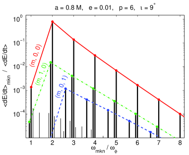
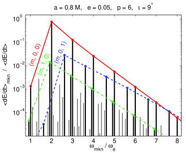
Figure 1: The dominant spectral lines for two relatively simple orbital configurations. The parameters describing the system (black hole spin $a$, eccentricity $e$, semilatus rectum $p$, and inclination $\iota$) are shown above each panel. For the spectrum on the left, 80% of the total power is carried by the dominant mode and 99% is carried by the most powerful 6 modes. For the spectrum on the right, 77% of the total power is carried by the dominant mode, and 99% is carried by the most powerful 11 modes. For each spectrum, 99.99% of the total power is carried by the lines shown. The red solid line traces over the tops of the lines carrying radiation at frequencies $\omega_{m00}=m\omega_{\phi}$, for various values of $m$ (which can be read off from the horizontal axis). Similarly, the green dash-dot line highlights frequencies $\omega_{m10}=m\omega_{\phi}+\omega_{\theta}$ (peaked at $m=1$), and the dashed blue line shows $\omega_{m01}=m\omega_{\phi}+\omega_{r}$ (peaked at $m=2$). The thicker spectral lines are members of these three mode families, while the thinner lines are not.

For both, the peak in the power spectrum occurs at a frequency of $2\omega_{\phi}$ as one might guess from, for example, the waveforms computed by Peters and Mathews using Newtonian orbits and the quadrupole formula peters mathews . The remaining power is distributed predominantly among three families of modes fixing the integer multipliers for the radial and azimuthal frequencies to be either zero or one. The frequencies for those mode families are

$$\omega=\left\{\begin{array}[]{ll}m\omega_{\phi}&\text{ dominant power at }m=2\\ m\omega_{\phi}+\omega_{r}&\text{ dominant power at }m=2\\ m\omega_{\phi}+\omega_{\theta}&\text{ dominant power at }m=1\end{array}\right.~{}.$$ (36)

From Fig. 1, one can see that the power in any given mode falls off exponentially with $m$, at a rate that is determined by both the orbit geometry, and the values of $k$ and $n$ that define the family. These mode families turn out to dominate the spectra for all orbits with sufficiently small eccentricity and inclination, and the exponential falloff for power in modes within a fixed family turns out to be a general trend for these simple spectra.

The distribution of power among modes or mode families is determined by the orbital geometry. The two panels of Fig. 1 show that increasing orbital eccentricity draws more power into the family involving the radial frequency, defined by modes (1b) with $(m,k,n)=(m,0,1)$. The spectrum from the system with higher orbital eccentricity also has the greater number of excited modes which are not members of the three families that dominate simple orbits. The following two sections will demonstrate that, in general, the complexity of the spectrum from any EMRI snapshot, or the number of modes excited by any fraction of the total power, is more sensitively dependent on eccentricity than on inclination or semilatus rectum.

This general rule that eccentricity governs spectral complexity is in accordance with the preliminary investigation of spectral dependence on orbit geometry given in Ref. drasco hughes 2006 . There, significant waveform “voices” were defined by sets of frequencies $\omega_{mkn}$ defined as follows

azimuthal voice: $$k=0\text{ and }n=0~{},$$ (37a)

polar voice: $$k\neq 0\text{ and }n=0~{},$$ (37b)

radial voice: $$k=0\text{ and }n\neq 0~{},$$ (37c)

mixed voice: $$k\neq 0\text{ and }n\neq 0~{}.$$ (37d)

For the spectra computed in Ref. drasco hughes 2006 , the distribution of power among these voices was more strongly dependent on eccentricity than on the other orbital parameters. From the spectra in Fig. 1, one might guess that these sets of frequencies are the best spectral classification scheme. The most significant of the mode families dominating simple spectra is exactly the azimuthal voice, and the other two dominant mode families are given by one member of either the radial or polar voices. For less simple orbits though, the voices defined above will prove a poor means of classifying spectra. For most generic orbit geometries, the bulk of the power is carried by the mixed voice, and there will prove to be a simple way of grouping the different members of that very large collection of modes.

The dominant lines of a third sample spectrum (also computed to a fractional accuracy of $\varepsilon_{\text{flux}}=10^{-6}$, in the total radiated power $\left<dE/dt\right>$) is shown in Fig 2.

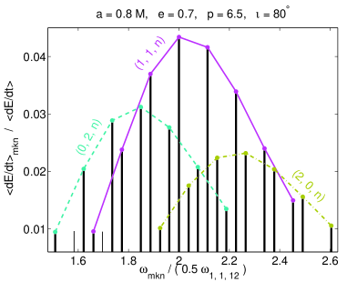
Figure 2: The dominant portion of the spectrum from a highly eccentric, and highly inclined, orbital configuration. The parameters describing the system (black hole spin $a$, eccentricity $e$, semilatus rectum $p$, and inclination $\iota$) are again shown at the top of the plot. For this spectrum, 4% of the total power is carried by the dominant mode, 99% is carried by the top 726 modes, and about 50% is carried by the lines shown. Here the highlighted mode families have frequencies $\omega_{11n}=\omega_{\phi}+\omega_{\theta}+n\omega_{r}$ (solid magenta line), $\omega_{02n}=2\omega_{\theta}+n\omega_{r}$ (dashed cyan line), $\omega_{20n}=2\omega_{\phi}+n\omega_{r}$ (dash-dot mustard-colored line), for various values of $n$. All but two of the shown lines are contained in these families (the two excluded lines are drawn slightly thinner than the others).

The orbit for this spectrum is both highly eccentric and highly inclined. The frequencies of the dominant modes are also not given by Eq. (36), but are instead

$$\omega=\left\{\begin{array}[]{ll}\omega_{\phi}+\omega_{\theta}+n\omega_{r}&\text{ dominant power at }n=12\\ 2\omega_{\theta}+n\omega_{r}&\text{ dominant power at }n=11\\ 2\omega_{\phi}+n\omega_{r}&\text{ dominant power at }n=14\end{array}\right.~{}.$$ (38)

These mode families are not easily classified by the voices (37) of Ref. drasco hughes 2006 . The values $n_{\max}$ of $n$ for the dominant members of these mode families can be crudely approximated (to within about 20% to 40% for the three families highlighted in Fig. 2) using the conjecture (6). Equation (6) is a good approximation to the peaks in the spectra derived by Peters and Mathews peters mathews

$$\left\langle\frac{dE}{dt}\right\rangle^{\text{PM}}_{\hat{n}}\!\! \propto\frac{{\hat{n}}^{4}}{32}\biggl{\{}\bigl{[}J_{{\hat{n}}-2}({\hat{n}}e)-2eJ_{{\hat{n}}-1}({\hat{n}}e)$$

$$+\frac{2}{{\hat{n}}}J_{\hat{n}}({\hat{n}}e)+2eJ_{{\hat{n}}+1}({\hat{n}}e)-J_{{\hat{n}}+2}({\hat{n}}e)\bigr{]}^{2}$$

$$+(1-e^{2})\left[J_{{\hat{n}}-2}({\hat{n}}e)-2J_{\hat{n}}({\hat{n}}e)+J_{{\hat{n}}+2}({\hat{n}}e)\right]^{2}$$

$$+\frac{4}{3{\hat{n}}^{2}}\left[J_{\hat{n}}({\hat{n}}e)\right]^{2}\biggr{\}},$$ (39)

where here $\hat{n}$ is the multiplier of the single frequency of a Newtonian orbit with eccentricity $e$, and $J_{\hat{n}}(x)$ are Bessel functions of the first kind. Though a very crude estimator for the values of $n$ describing the dominant members of various mode families, this formula is better than any other estimator that has been tried in the present work.

By comparison to the simple spectra, the number of modes needed to capture any fraction of the total power from the complicated spectrum is much larger. This is demonstrated more clearly by Fig. 3.

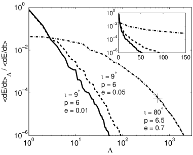
Figure 3: The normalized mode amplitudes for the orbital configurations whose corresponding spectra are shown in Figs. 1 and 2, sorted in order of decreasing power. The parameters describing the orbital geometry (eccentricity $e$, semilatus rectum $p$, and inclination $\iota$) are shown next to each curve. The crosshairs shown on the solid curve indicate the location of the mode with frequency $\omega=2\omega_{\phi}$. That same mode is the dominant mode for both of the other systems, as can be read off of Fig. 1. The inset plot shows the same curves, but on a log-linear scale over a shorter range.

There one can see that, when the modes of a given spectra are sorted by mode number $\Lambda$ in order of decreasing power, mode power falls off roughly as a power law $\Lambda^{\alpha}$, where $\alpha$ is orbit dependent, for the simple orbits. For the two simple orbits, the rate of this power-law falloff is faster for the less eccentric orbit. If there is a power-law falloff for the more complicated orbit, it is not evident in the first thousand modes. However, given that the essentially blind algorithm from Ref. drasco hughes 2006 computed $\approx$ 30,000 modes before finding the dominant thousand or so shown for the complicated orbit in Fig. 3, most of the total power is still captured by a surprisingly small number of modes.

Note also that the mode which dominates the simple orbits, with frequency $2\omega_{\phi}$, hardly contributes to the spectrum of the complicated orbits. In Fig. 3, the location of that mode on the curve for the complicated orbit is indicated with a crosshairs at about $\Lambda=600$, and its power relative to the total power $\approx 6\times 10^{-5}$, is effectively insignificant. This is an extreme example of an effect that has been noticed in simulations of black hole binary inspirals with mass ratios near unity. In the language of post-Newtonian descriptions of such systems (for a recent overview see Ref. van den broeck and sengupta ) all modes other than the one with frequency $2\omega_{\phi}$ are “higher harmonics.” The excitation of higher harmonics in those systems has been found to be significant in both analytic parameter estimation studies for LISA sintes vecchio ; hellings moore ; arun et al ; arun et al 2 ; trias sintes and fully relativistic numerical simulations berti et al 2007 ; vaishnav et al . LISA parameter estimation studies have to date included either spin precession effects cutler ; vecchio ; berti buonanno will ; lang hughes or higher harmonics hellings moore ; arun et al ; trias sintes , but not yet both.

IV Survey of many spectra

In this section, I simulate EMRI snapshots for a large grid of orbital parameters and discuss how the spectral trends identified in the previous section vary over the grid. For each snapshot in the survey, the spin of the large black hole is taken to be $a=0.8M$, and the spectra are computed with the code described in Ref. drasco hughes 2006 using a requested fractional accuracy of $\varepsilon_{\text{flux}}=1\%$, in the total radiated power $\left<dE/dt\right>$. The grid of orbital parameters is uniformly spaced in eccentricity $e$, inclination $\iota$, and in the ratio of the semilatus rectum $p$ to its value for the innermost stable circular orbit (ISCO) $p_{\text{ISCO}}$. The specific values for these parameters are given in Table 1.

$e$	$p$	$\iota$	$e$	$p$	$\iota$
0.1	3.4880	20∘	0.1	10.118	110∘
0.1444	3.7632	25.556∘	0.1444	10.917	115.56∘
0.1889	4.0388	31.111∘	0.1889	11.716	121.11∘
0.2333	4.3140	36.667∘	0.2333	12.514	126.67∘
0.2778	4.5893	42.222∘	0.2778	13.313	132.22∘
0.3222	4.8648	47.778∘	0.3222	14.112	137.78∘
0.3667	5.1401	53.333∘	0.3667	14.911	143.33∘
0.4111	5.4157	58.889∘	0.4111	15.710	148.89∘
0.4556	5.6909	64.444∘	0.4556	16.509	154.44∘
0.5	5.9662	70∘	0.5	17.307	160∘
0.54	6.2417		0.54	18.106
0.58	6.5170		0.58	18.905
0.62	6.7922		0.62	19.703
0.66	7.0678		0.66	20.503
0.7	7.3431		0.7	21.301
0.74	7.6186		0.74	22.101
0.78	7.8939		0.78	22.899
0.82	8.1691		0.82	23.698
0.86	8.4447		0.86	24.497
0.9	8.7199		0.9	25.295

Table 1: The parameters characterizing the 8000 orbit geometries considered (all about a black hole with spin $a=0.8M$). The prograde ($\iota<90^{\circ}$) are characterized by the 4000 possible combinations of the first three columns, and the retrograde ($\iota>90^{\circ}$) are characterized by the 4000 possible combinations of the last three columns. The two different ranges for $p$ correspond to one uniform range for $p/p_{\text{ISCO}}$. See Fig. 4 for a graphical representation of the stable orbits. Note that, for prograde ($\iota<90^{\circ}$) orbits, $p_{\text{ISCO}}\approx 2.9066$. Retrograde ($\iota>90^{\circ}$) orbits have a less relativistic $p_{\text{ISCO}}\approx 8.4318$.

Of the 8000 orbit geometries shown in Table 1, 728 are unstable. For the unstable orbits, the derivative of the radial potential is negative at the prescribed minimum radius

$$\left.\frac{d}{dr}\left(\frac{dr}{d\lambda}\right)^{2}\right|_{r_{\min}}<0~{},$$ (40)

where $\lambda$ is Mino’s time parameter, related to proper time $\tau$ by $d\tau=(r^{2}+a^{2}\cos^{2}\theta)d\lambda$, and where the radial potential is

$$\left(\frac{dr}{d\lambda}\right)^{2}=\left(E\varpi^{2}-aL\right)^{2}-\Delta\left[\mu^{2}r^{2}+(L-aE)^{2}+Q\right]~{}.$$ (41)

Here $\varpi^{2}=r^{2}+a^{2}$ and $\Delta=r^{2}-2Mr+a^{2}$. Snapshot spectra were computed for each of the remaining 7272 stable orbital configurations, represented graphically in Fig. 4. The total computational cost of simulating these spectra was about 2.7 CPU-years on a machine based on a 3.2 GHz Intel Pentium 4 Xeon processor.

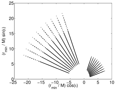
Figure 4: A graphical representation of the stable orbits described by the parameters shown in Table 1. The inclination and minimum radius ($r_{\min}$) for the 7,272 stable orbits are shown.

All of the spectra from this grid are dominated by mode families characterized by frequencies

$$\omega=\left\{\begin{array}[]{l}\pm 2\omega_{\phi}+n\omega_{r}\\ \pm\omega_{\phi}+\omega_{\theta}+n\omega_{r}\end{array}\right.~{},$$ (42)

where $\pm$ was 1 for prograde orbits and $-1$ for retrograde orbits. To within an error on the order of 10%, the most dominant mode for either family had $n=n_{\max}$, where $n_{\max}$ is given by the Peters-Mathews approximation (6). The success of that approximation remains similar to that for the more complicated sample spectrum in Fig. 2, and is plotted for the entire set of orbits in Fig. 5.

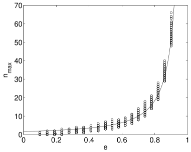
Figure 5: The circles indicate the value of $n$ in $\omega_{mkn}$ for the most powerful modes in the spectra from the stable orbits in Table 1. The solid curve is the approximation (6) that gives the peaks in the approximate spectra (III) derived for Newtonian orbits by Peters and Mathews peters mathews .

Of the two dominant mode families (42) the first one, with $(m,k,n)=(2,0,n)$, is the most common. The exceptions, dominated by the $(1,1,n)$-family, are the orbits with $\iota$ nearest to 90^∘. This trend is demonstrated in Table 2.

$\iota$	Fraction of orbits
20∘	0
25.556∘	0
31.111∘	0
36.667∘	0
42.222∘	0
47.778∘	0
53.333∘	0
58.889∘	26%
64.444∘	94%
70∘	100%
110∘	100%
115.56∘	100%
121.11∘	100%
126.67∘	100%
132.22∘	1.8%
137.78∘	0.3%
143.33∘	0.3%
148.89∘	0.3%
154.44∘	0.3%
160∘	0.3%

Table 2: The fraction of orbits, from the grid of orbits described in Table 1, dominated by a mode with frequency $\omega_{mkn}$, where $(m,k,n)=(\pm 1,1,n)$, as a function of inclination $\iota$. The remaining orbits are dominated by modes with $(m,k,n)=(\pm 2,0,n)$. Here $\pm$ is $1$ for prograde orbits ($\iota<90^{\circ}$) and $-1$ for retrograde orbits ($\iota>90^{\circ}$). Note that since the grid of orbits is uniformly spaced in $p/p_{\text{ISCO}}$, rather than in $p$, the prograde orbits have smaller values for $p$ than do the retrograde orbits.

The prograde orbits tend to be less easily dominated by the $(1,1,n)$ family. Since the orbit grid is evenly spaced in $p/p_{\text{ISCO}}$, and since $p_{\text{ISCO}}$ is much smaller for prograde orbits than for retrograde orbits, this suggests that the closer the orbit comes to the horizon, the harder it becomes for the system to channel radiation away from the $(2,0,n)$-family and into the $(1,1,n)$ family.

As with the sample orbits, the number of modes needed to capture the bulk of the radiated power remains resonably small. This is shown in Fig. 6 by a histogram of the number of modes $N_{99\%}$ carrying 99% of the power.

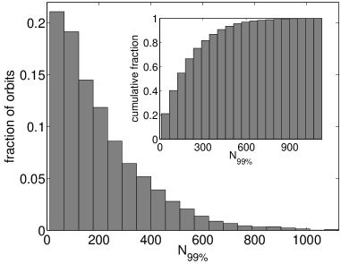
Figure 6: A histogram showing the fraction of orbits, out of the 7,272 stable orbits in Table 1, for which $N_{99\%}$ modes are required to capture 99% of the radiated power. The inset displays the same data as a cumulative distribution (its vertical axis showing the fraction of orbits with $N_{99\%}$ less than the value on the horizontal axis).

An example of the dependence of $N_{99\%}$ on orbit geometry is plotted in Fig. 7.

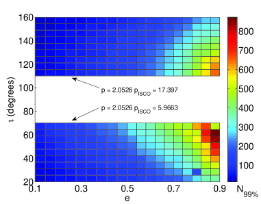
Figure 7: The number of modes required to capture 99% of the radiated power, $N_{99\%}$, as a function of eccentricity $e$ and inclination $\iota$ for a fixed value of $p/p_{\text{ISCO}}$. Since $p_{\text{ISCO}}$ is larger for retrograde orbits, the top block of this plot corresponds to orbits with larger values of $p$.

That plot shows the values of $N_{99\%}$ for all the orbits with the smallest value of $p/p_{\text{ISCO}}$, such that over the grid’s range for the other orbital parameters, no orbits were unstable.

It is important to emphasize that the values of $N_{99\%}$ given in this and the following section are accurate only to $\sim 10\%$. This is because $N_{99\%}$ is found only after the algorithm from Ref. drasco hughes 2006 computes a much larger number of modes $N$ in an effort to determine the total power to its requested fractional accuracy of $\varepsilon_{\text{flux}}=1\%$. Once that algorithm terminates, the modes that it computed are sorted in order of decreasing power such that

$$\left<\frac{dE}{dt}\right>=\sum_{\Lambda=1}^{N}\left<\frac{dE}{dt}\right>_{\Lambda}~{},$$ (43)

where $\left<dE/dt\right>_{\Lambda}$ decreases with $\Lambda$. The value of $N_{99\%}$ is the smallest possible value satisfying

$$\sum_{\Lambda=N_{99\%}}^{N}\left<\frac{dE}{dt}\right>_{\Lambda}<(0.01)\left<\frac{dE}{dt}\right>~{}.$$ (44)

Spot checking its dependence on $\varepsilon_{\text{flux}}$ for a few sample spectra gave an expected accuracy $\sim 10\%$.

Figure 7 also shows that, as with the sample orbits, $N_{99\%}$ is more strongly dependent on eccentricity than on inclination and semilatus rectum. This is especially significant for the prospect of observing intermediate mass ratio inspirals with ground-based detectors like LIGO, since the systems that have been estimated to be the most likely candidates for being observed are those with especially small eccentricity, typically $e<10^{-4}$ and at most $e\approx 0.1$ mandel et al 2007 . For LIGO, it is likely that waveforms needed for detection need only contain a few to $\sim 10$ modes. This both simplifies LIGO’s task of detection, since the waveform snapshots will not be very complicated, and hardens its task of spacetime mapping, since correspondingly less information will be observable.

V Spectra from a kludged inspiral

In this section, I describe how general spectral characteristics should be expected to evolve during an EMRI. The snapshots studied here will be sampled at approximately 12-hour intervals over the final three years of a single kludged EMRI thought to be typical of the kind that could be observed by LISA. The kludged trajectory through orbital parameter space $e(t)$, $\iota(t)$, and $p(t)$, was provided by Jonathan Gair, and was numerically computed according to the prescription introduced in Ref. gair glampedakis 2005 . Their method for approximating the trajectory is based on an eclectic combination of approximations including post-Newtonian equations for the radiative fluxes of energy and angular momentum, numerical fits to Teukolsky-based calculations of fluxes for circular and equatorial orbits, as well as some uncontrolled approximations for the evolution of Carter’s constant. Since only power spectra will be discussed here, the results are independent of any evolution for the positional orbital elements, or $\chi_{mkn}$ in Eq. (34). While one would expect minimal accuracy from such an array of approximations, these kludged trajectories have been shown to exhibit a stunning degree of agreement with more accurate calculations. The integrated overlap between approximate waveforms based on the kludged orbit trajectories and waveforms constructed from black hole perturbation theory alone is often about 95% babak et al 2007 . So a kludged orbit trajectory is likely more than adequate for the present purpose, since the snapshots themselves will still be accurate up to leading order in the mass ratio, and since for the majority of the spectra examined in the previous section, the general character of a spectrum does not change dramatically for small perturbations to the orbital parameters.

The kludged orbit trajectory for the inspiral examined here is shown in Fig. 8

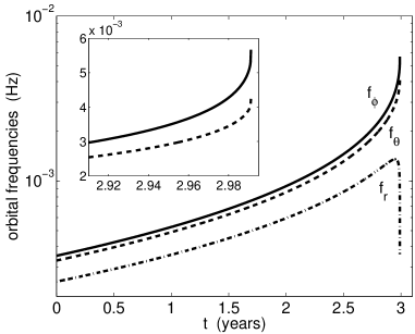
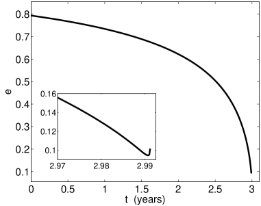
Figure 8: The kludged evolution for a selection of the orbits principal elements during an inspiral of the sort that could be observed with LISA. For this system, the large black hole has mass $M=10^{6}M_{\odot}$, and the magnitude of its spin angular momentum is $a=0.9M$. The smaller black hole is nonspinning and has mass $\mu=10M_{\odot}$. The initial orbit has eccentricity $e=0.79$, semilatus rectum $p=8.8$, and inclination $\iota=43^{\circ}$. The final orbit has eccentricity $e=0.10$, semilatus rectum $p=3.2$, and inclination $\iota=45^{\circ}$. The orbit trajectory $e(t)$, $p(t)$, and $\iota(t)$ for this inspiral was computed by Jonathan Gair using the algorithm described in Ref. gair glampedakis 2005 . The approximations used to compute the trajectory should become less accurate with time as the system becomes increasingly relativistic. The top panel shows the evolution of the orbital frequencies $f_{r,\theta,\phi}=\omega_{r,\theta,\phi}/(2\pi)$ with an inset of the same but over a different range. The bottom panel shows the evolution of orbital eccentricity $e$, with an inset of the same but over a different range.

The principal orbital elements evolve slowly and smoothly throughout the majority of the inspiral. In the final few days of the inspiral, where the trajectory should be least accurate and where the adiabatic approximation itself should begin to fail, the eccentricity begins to rise with time, and the orbital frequencies rapidly diverge from each other. The trajectory ends when it has evolved onto an unstable orbit, at which point the binary would merge to form a single black hole.

Snapshot spectra were computed at roughly 12-hour intervals along the orbit trajectory in Fig. 8. As was done for the grid of spectra in the previous section, these spectra were computed with the code described in Ref. drasco hughes 2006 using a requested fractional accuracy of $\varepsilon_{\text{flux}}=1\%$, in the total power $\left<dE/dt\right>$. There were 2,143 snapshots in all, and the total computational cost of simulating them was about 1.5 CPU-years on a machine based on a 3.2 GHz Intel Pentium 4 Xeon processor. The initial and final snapshot spectra from this sequence are shown in Fig. 9.

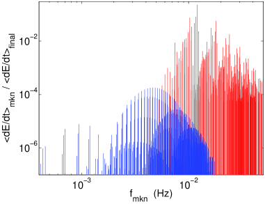
Figure 9: The initial (blue, or dark grey) and final (red, or light grey) power spectra for the inspiral shown in Fig. 8. An animated movie of the complete spectral evolution is available upon request.

The inspiral’s initial spectrum is similar in character to the one shown in Fig. 2, due to the large initial orbital eccentricity. The final spectrum is more similar to the ones in Fig. 1. The dominant mode families for both the initial and final spectra have $(m,k,n)=(2,0,n)$ and $(1,1,n)$. Those two families make up the two largest arcs or lobes of lines in the initial spectrum. In the final spectrum, the lobes are much more narrow, and are not as easily identified by eye. For the final spectrum, a more efficient definition of mode families might instead use $m$ as the free index, rather than $n$. For example, the strongest lines along the upper right edge of the final spectrum are $(m,0,m)$, peaked at $m=2$.

Figure 10 shows the evolution in spectral complexity during the inspiral.

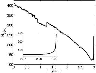
Figure 10: The evolution of the number of modes needed to capture 99% of the radiated power $N_{99\%}$ for the inspiral shown in Fig. 8. The inset shows a close-up view over about the last week of the inspiral.

As the binary becomes more circular, the number of lines carrying 99% of the spectral power $N_{99\%}$ decreases with time until the last few days, at which point both the kludge and adiabatic approximations should fail. Over those last few days the orbital eccentricity rises and $N_{99\%}$ jumps from about 125 to 250. This effect is typical of both kludged trajectories and the more accurate Teukolsky-based trajectories. While it may be a physical effect, it always occurs suspiciously in regimes where the adiabatic approximation and kludge should be least accurate. The question of whether or not it is physical might best be addressed by the numerical relativity community. The causes of the smaller abrupt jumps in $N_{99\%}$ (for example, at either end of a six month gap centered at about one year) is unknown, however, they are within the expected accuracy $\sim 10\%$ whereas the final jump from 125 to 250 is not. Repeating the snapshot calculations with a smaller requested overall accuracy in the total power $\varepsilon_{\text{flux}}$ would likely eliminate most, if not all, of these small jumps.

VI Verification of black hole orbits

In this section I suggest EMRI detection algorithms based on the spectral trends found above and discuss the scientific meaning of successful detections. The tone of the discussion is meant to be exploratory rather than exhaustive. That is, it is meant to outline the sorts of data analysis strategies that the simulations described above suggest would be useful, rather than to look in great detail at any one algorithm.

This section will be divided up into two subsections. The first subsection outlines algorithms that could search for systems without radiation reaction. These are really just of interest as building blocks for more complicated searches since only a small subset of EMRIs would be observable without accounting for the influence of radiation on the binary. The second subsection describes how these building blocks would be used to search for realistic systems affected by radiation reaction and gives a detector-independent estimate of how well these algorithms might perform in the best of circumstances.

VI.1 Without radiation reaction

For times that are sufficiently short for the orbit of the captured mass to be unaffected by radiation, the general expression for EMRI snapshots (1) is accurate up to corrections that are at most of order $\mu^{2}/M^{2}$ and are perhaps even as small as $\sim\mu^{3}/M^{3}$ with the principal frequencies adjusted according to the second order metric perturbation mino 2007 . In this subsection, I will outline a detection strategy for a signal of this form. Truncating the general expression for an EMRI-snapshot waveform (1) to a finite number of $N$ modes, rewriting it as a single sum, and explicitly showing the positional phase elements, gives the following

$$h_{+}-ih_{\times} = \sum_{\Lambda=1}^{N}h_{\Lambda}\exp\left\{-i[m_{\Lambda}\omega_{\phi}(t-t_{\phi})\right.$$ (45)

$$+ \left.k_{\Lambda}\omega_{\theta}(t-t_{\theta})+n_{\Lambda}\omega_{r}(t-t_{r})]\right\}~{}.$$

I wish to consider the prospects of using this truncated expression (45) explicitly as a phenomenological template.

By phenomenological templates, I mean templates for which some of the free and measurable parameters will have no immediately obvious physical meaning. Traditional, or nonphenomenological templates are constructed as follows. You start by declaring the 17 parameters which completely determine the waveform (e.g. the two masses, and 3-vectors for the position and velocity of each object as well as for the spin of the larger object). You then solve Einstein’s equation or some perturbed form of it to completely determine $h_{+,\times}$. This last step is equivalent to determining all of the frequencies $\omega_{r,\theta,\phi}$, phase shifts $t_{r,\theta,\phi}$, and Fourier coefficients $h_{\Lambda}$ in the model (1). The phenomenological templates are computed in a much simpler way. You first chose values for the frequencies, phase shifts, and Fourier coefficients, and then you simply evaluate the sum over modes (45). For these waveforms, the frequencies, phase shifts, and Fourier coefficients are themselves the free quantities to be measured. For a phenomenological template with $N$ modes, there are then $5N+6$ free parameters. Of those there are $2N+6$ real numbers (the three frequencies, the three phase shifts, and the $N$ complex mode amplitudes), as well as $3N$ integers (the frequency multipliers $m_{\Lambda}$, $k_{\Lambda}$, and $n_{\Lambda}$).

The most obvious objection to the use of these phenomenological templates in gravitational wave searches is the large dimensionality of the parameter space. For templates that allow for any more than $N=2$ modes, you will have more free parameters than the traditional templates, and of those only the three frequencies $\omega_{\phi,\theta,r}$ will carry immediate physical meaning. In the traditional scheme, however, the step of going from the complete set of 17 parameters to the waveform is extremely costly. Since both template families are equally good matches to the true waveforms, and since either way you will be dealing with a significant number of template parameters, it may be worth adding dimensionality to the template parameter space in exchange for not having to solve Einstein’s equation.

Though the large dimensionality may seem daunting, especially for those familiar with efforts focused on sources with just a few degrees of freedom, it is not unrealistic for elaborate algorithms to identify signals characterized by a large number of parameters. For algorithms that match against templates over a sequence of increasingly dense grids on the model parameter space, computational cost grows as a power law where the power is proportional to the number of free parameters. Algorithms designed for more complex models have costs that instead grow only linearly with the number of parameters. Algorithms of this nature have been used in the mock LISA data challenges mldc to recover $\sim 10^{4}$ white dwarf binaries.

I now discuss how well phenomenological detection algorithms can be expected to perform in the best case scenario where the algorithm has no difficulty in selecting the correct parameter values. This can be done without reference to specific instruments, and in a sky averaged sense, by studying the distribution of the power among various modes relative to the total power radiated by the binary. More sophisticated estimates that account for detector characteristics and variation of signal parameters are certainly possible, but they are beyond the scope of this paper.

For the task of searching only for EMRI snapshots with phenomenological templates, the example spectra from Sec. III suggest estimates of the minimum scale of the phase space dimensionality. For example, systems with eccentricities of about 1% will produce spectra similar to Fig. 1. So a ground-based phenomenological search for these systems would require $N\lesssim 10$ modes, resulting in a model with 56 parameters (26 real numbers and 30 relatively small integers). For snapshots thought to be typical of EMRIs that could be observed with space-based detectors, one would need $N\sim 10^{2}$ to $10^{3}$. This would mean a model with about 500 to 5000 free parameters, still far fewer than what has been demonstrated already for white dwarf binaries mldc .

If a search for phenomenological EMRI snapshots were successful, only the general waveform model would be verified. One would only be able to claim detection of some signal with a discrete triperiodic spectrum with some measured fundamental frequencies $\omega_{\phi,\theta,r}$, since the physical meaning of the other unknown parameters is convoluted. In this event, one could then turn to the underlying physical model. Finding a set of its 17 free parameters that best reproduce the parameters measured in the phenomenological search would then confirm the physical model to some more explicit level of uncertainty. Failing to find parameters for the underlying physical model might mean that the snapshot was produced by a test mass moving along a geodesic of some non-Kerr spacetime, since many (but not all) candidates for such orbits are also triperiodic gair li mandel 2007 ; flanagan hinderer 2007 .

Some intermediate level of model verification is also possible and could reduce the dimensionality of the parameter space for the phenomenological templates. For example, sixteen mode families are needed to capture 99% of the power radiated by the initial snapshot from the inspiral examined in the previous section. The distribution of power among these families is shown in Table 3.

$m$	$k$	$n_{\max}$	$\left<\dot{E}\right>_{mk}/\left<\dot{E}\right>$
2	0	16	5.1$\times 10^{-1}$
1	1	15	2.2$\times 10^{-1}$
3	0	27	9.2$\times 10^{-2}$
2	1	25	6.2$\times 10^{-2}$
0	2	13	3.5$\times 10^{-2}$
4	0	38	2.0$\times 10^{-2}$
1	2	24	1.7$\times 10^{-2}$
3	1	36	1.8$\times 10^{-2}$
2	2	35	6.4$\times 10^{-3}$
2	-1	12	3.7$\times 10^{-3}$
4	1	47	2.9$\times 10^{-3}$
5	0	49	2.5$\times 10^{-3}$
-1	3	12	1.9$\times 10^{-3}$
0	3	22	1.3$\times 10^{-3}$
3	2	45	1.5$\times 10^{-3}$
3	-1	21	9.9$\times 10^{-4}$

Table 3: The 16 mode families needed to capture 99% of the power radiated during the first 12 hours of the inspiral discussed in Sec. V. Each family is defined by fixing $m$ and $k$. The most powerful member of each family has frequency $m\omega_{\phi}+k\omega_{\theta}+n_{\max}\omega_{r}$. The ratio of the power radiated by each family to the total power from this first 12 hours is given by $\left<\dot{E}\right>_{mk}/\left<\dot{E}\right>$. For this system, the spin of the black hole is $a=0.9M$, and the orbit of the test mass has eccentricity $e=0.79$, semilatus rectum $p=8.8$, and inclination $\iota=43^{\circ}$.

As is true for all the snapshots simulated in this paper, this one is dominated by the mode families with $(m,k,n)=(2,0,n)$ and $(1,1,n)$. And as is typical, those two mode families carry most of the power, 73% here. In an effort to simplify the phenomenological waveform model, one might restrict it to include only those mode families. This specific model would eliminate ($m_{\Lambda}$, $k_{\Lambda}$) from the template parameter space by fixing them to either $(2,0)$ or $(1,1)$, and would create two new parameters specifying the number of modes in each of the two families. This would reduce the number of free parameters from $5N+6$ to $3N+8$.

VI.2 With radiation reaction

The scenario describe in the previous subsection is only immediately useful for EMRI’s with the most extreme mass ratios. There is no compelling reason to expect those systems to be especially common, or to even consider them reasonable targets at all. The purpose of studying these simple systems is to construct from the results an approximate description of more generic EMRIs that respond to their own radiation. That is, we wish to describe the radiation of a generic adiabatic EMRI as a slowly evolving sequence of EMRI snapshots. Here I will now outline how the phenomenological templates for EMRI snapshots could be modified to describe the more general class of adiabatic EMRIs. There are many ways that this could be done. Although a detailed study of specific models would be valuable, it is beyond the scope of this paper. Instead, I aim to be as general as possible and will steer away from discussing any specific implementation.

For an adiabatic EMRI, the motion of the small object is described by a solution of the geodesic equation for the Kerr spacetime, but with the orbital elements replaced by quantitates that evolve slowly. The Teukolsky equation can provide the leading order radiative changes to those quantities, and more sophisticated techniques are envisioned for describing both conservative and radiative effects. In the spirit of trading calculation difficulty for added dimensionality, every quantity that was constant for the snapshot model (45) could in principle be replaced by simple, one or two parameter models.

To illustrate this, consider the orbital frequencies $\omega_{i}$, for $i=r$, $\theta$, $\phi$. These can be taken to drift linearly with time

$$\omega_{i}\to\omega_{i}+\dot{\omega}_{i}t~{}.$$ (46)

where I have introduced new constants $\dot{\omega}_{i}\propto\mu/M$. This simple model fits the first year of the three frequency trajectories shown in Fig. 8 with an average fractional accuracy of about 1%. Other models can of course do better. For example, Peters and Mathews derived an expression for radius as a function of time in the case of slow circular inspirals. Combining that result, Eq. (5.9) of Ref. peters mathews , with Kepler’s law $M\omega=(r/M)^{-2/3}$, gives

$$M\omega=\left[\left(\frac{r_{0}}{M}\right)^{4}-\frac{256}{5}\frac{\mu}{M}\frac{t}{M}\right]^{-3/8}~{}.$$ (47)

For the more general case of fast generic motion, one might want to try a model with a similar form

$$M\omega_{i}=[\alpha_{i}+\beta_{i}(t/M)]^{-\gamma_{i}}~{}.$$ (48)

This model fits the first year of the three frequency trajectories shown in Fig. 8 with $\gamma_{i}\approx 1.6$ and an average fractional accuracy on the order of $10^{-4}$. It performs similarly at later times, but not with the same values of the parameters $\alpha_{i}$, $\beta_{i}$, and $\gamma_{i}$. Unlike the simple linear model however, this one has three parameters instead of two.

To complete the construction of phenomenological templates for adiabatic EMRIs, similar models can be concocted for the other parameters of the snapshot templates (45), the complex mode amplitudes, and the positional phase elements. If one-parameter models like the linear frequency drift are used, then the new template is given by Eq. (45) with

$$h_{\Lambda} \to h_{\Lambda}+\dot{h}_{\Lambda}t~{},$$ (49)

$$m_{\Lambda} \to m_{\Lambda}+\dot{m}_{\Lambda}t~{},$$ (50)

$$k_{\Lambda} \to k_{\Lambda}+\dot{k}_{\Lambda}t~{},$$ (51)

$$n_{\Lambda} \to n_{\Lambda}+\dot{n}_{\Lambda}t~{},$$ (52)

$$\omega_{i} \to \omega_{i}+\dot{\omega}_{i}t~{}.$$ (53)

$$t_{i} \to t_{i}+\dot{t}_{i}t~{},$$ (54)

again for $i=r$, $\theta$, $\phi$. For this case, the dimensionality of the template parameter space is doubled to $10N+12$. Of those, only the $3N$ frequency multipliers are integers. These phenomenological templates are similar in nature to the time-frequency search methods which have been successfully demonstrated in the mock LISA data challenge gair et al 2007 . They differ from those in that they can accommodate coherent integration and could also more naturally include specific schemes for evolving both the principle and positional orbital elements.

Given that EMRI snapshots tend only to be dominated by a small number of mode families, it is likely that a slightly simpler waveform model could be used for adiabatic EMRIs. Figure 11 demonstrates how successful two such hypothetical detection algorithms might be if searching for the kludged inspiral from Sec. V.

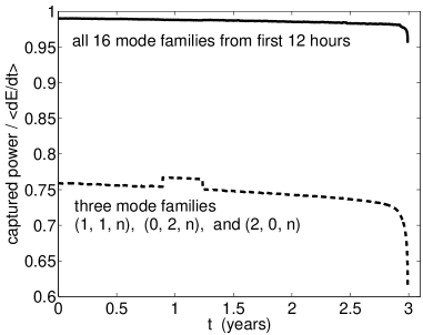
Figure 11: A time-dependent measure of success for two hypothetical detection algorithms searching for the inspiral from Fig. 8. The algorithm for the dashed blue curve captures the power radiated at all frequencies of the form $\omega_{mkn}$, where $(m,k,n)=(1,1,n)$, $(0,2,n)$, and $(2,0,n)$, for any $n$. The solid curve captures power radiated at all frequencies in the 16 mode families needed to capture 99% of the initial power, where here a mode family is defined as all modes with frequencies $\omega_{mkn}$ for some fixed $m$ and $k$.

If one were to search for this waveform using a model that included only the dominant three mode families from the sample complicated snapshot in Fig. 2 one would recover $71\%$ of the inspiral’s total power. Assuming this could be done with one-parameter models for the adiabatic evolution of the waveforms parameters, such a model would have $6N+18$ free parameters (by eliminating $2N$ frequency multipliers and their $2N$ linear drifts, and by adding three new integers specifying how many modes are in each family, as well as their three linear drifts). For this example EMRI, this scheme included $N=121$ modes. So 714 free parameters would have been needed to recover 71% of the power. A similar hypothetical algorithm which captured all the power carried by the 16 mode families that make up most of that inspiral’s initial spectrum (Table 3) would recover 98% of the total power with $6N+44$ free parameters (by eliminating $2N$ frequency multipliers and their $2N$ linear drifts, and by adding 16 new integers specifying how many modes are in each family, as well as their 16 linear drifts). For this example EMRI, this scheme included $N=411$ modes. So 2,510 free parameters would have been needed to recover 98% of the power.

It should be emphasized that any gravitational wave detections following from the use of these phenomenological waveform models would not necessarily yield either the parameters that completely determine an EMRI (position, masses, etc) or the spacetime map that general relativity predicts is encoded in the radiation. They would however verify the detection of waveforms predicted to be produced when a test mass perturbs a rotating black hole by moving through an adiabatic sequence of its bound geodesic orbits. They would also measure the evolution of the three fundamental frequencies throughout that sequence, or equivalently the evolution for any other set of principle orbital elements. It is possible that restricting phenomenological EMRI waveforms to include only the mode families that are most commonly dominant in the snapshots simulated here may alone be enough of a constraint to keep EMRIs into non-Kerr black hole candidates from triggering a detection. However, without more work with the snapshots from such EMRIs one could not say so with any certainty. One would have to be content only to have verified that radiation from an adiabatic sequence of black hole orbits could have triggered the detection.

VII Conclusion

The number of significant modes in generic EMRI-snapshot spectra has been shown generally to be much more manageable than one might have guessed from earlier truncation algorithms drasco hughes 2006 . This should lead to improved truncation algorithms, which will reduce the cost of future data analysis efforts. Such improvements should exploit the trends observed here in the relationship between orbit geometry and spectral signature. The ability to predict the multiplier $n\approx n_{\max}$ of the radial frequency for the dominant modes using a formula based on such simple approximations peters mathews is encouraging. It suggests that many of the trends in these spectra might be understood analytically using more recent tools moreno-garrido mediavilla buitrago ; poisson ; ganz et al .

The detection algorithms that are suggested here for verifying minimal aspects of relativity and black hole physics may ultimately be used in future gravitational wave detections. However, more work is needed to determine whether or not they are cost-efficient and science-efficient alternatives to traditional search techniques. Another possibly interesting area for future work is to explore the dependence of the snapshot spectra on the spin of the larger black hole. It has been implicitly assumed that the large values of spin considered are somehow representative of observable EMRIs. This is reasonable since the few existing measurements due to modeling x-ray spectra from galactic nuclei suggest near-maximal spins miller ; reis et al . Still, future work that tests the generality of these parameter values by simulating other EMRIs would be worthwhile.

Appendix A Bi periodic form of time-dependent spatial coordinates

Here I derive the bi-periodic form (9) of the spatial Boyer-Lindquest coordinates $r$, $\theta$, and $\phi$ for bound geodesics as a function of the time coordinate $t$.

The bi-periodic forms of both the radial and polar coordinates follows immediately from Sec. IV of Ref. drasco hughes 2004 by replacing $f[r(t),\theta(t)]$ with $r(t)$ and $\theta(t)$. The resulting relationships between the coefficients in the Mino-time series expansion (7) and the coordinate-time expansions (9) are given by

$${\tilde{r}_{kn}} = \frac{\Upsilon_{r}\Upsilon_{\theta}}{(2\pi)^{2}\Gamma}\int_{0}^{2\pi/\Upsilon_{r}}d\lambda_{r}\int_{0}^{2\pi/\Upsilon_{\theta}}d\lambda_{\theta}$$ (55)

$$\times \frac{dt}{d\lambda}[r(\lambda_{r}),\theta(\lambda_{\theta})]e^{i(k\omega_{\theta}+n\omega_{r})\delta t(\lambda_{r},\lambda_{\theta})}$$

$$\times r(\lambda_{r})e^{ik\Upsilon_{\theta}\lambda_{\theta}+in\Upsilon_{r}\lambda_{r}}~{},$$

$${\tilde{\theta}_{kn}} = \frac{\Upsilon_{r}\Upsilon_{\theta}}{(2\pi)^{2}\Gamma}\int_{0}^{2\pi/\Upsilon_{r}}d\lambda_{r}\int_{0}^{2\pi/\Upsilon_{\theta}}d\lambda_{\theta}$$ (56)

$$\times \frac{dt}{d\lambda}[r(\lambda_{r}),\theta(\lambda_{\theta})]e^{i(k\omega_{\theta}+n\omega_{r})\delta t(\lambda_{r},\lambda_{\theta})}$$

$$\times \theta(\lambda_{\theta})e^{ik\Upsilon_{\theta}\lambda_{\theta}+in\Upsilon_{r}\lambda_{r}}~{},$$

where $r(\lambda_{r})$ and $\theta(\lambda_{\theta})$ are given by their Mino-time series expansions with $\lambda=\lambda_{r}$ and $\lambda=\lambda_{\theta}$, respectively,

$$r(\lambda_{r})=\sum_{n}r_{n}e^{-i\Upsilon\lambda_{r}}~{}, \theta(\lambda_{\theta})=\sum_{k}\theta_{k}e^{-i\Upsilon\lambda_{\theta}}~{},$$ (57)

and where

$$\delta t(\lambda_{r},\lambda_{\theta})=\sum_{kn}t_{kn}e^{-ik\Upsilon_{\theta}\lambda_{\theta}-in\Upsilon_{r}\lambda_{r}}~{}.$$ (58)

The $\lambda$-derivative of $t$ can be evaluated analytically as given by Carter’s first order geodesic equations, or it can be found from

$$\frac{dt}{d\lambda}[r(\lambda_{r}),\theta(\lambda_{\theta})] =\Gamma$$

$$-i\sum_{kn}(k\Upsilon_{\theta}+n\Upsilon_{r})t_{kn}e^{-ik\Upsilon_{\theta}\lambda_{\theta}-in\Upsilon_{r}\lambda_{r}}~{}.$$ (59)

The derivation of the bi periodic form for $\phi(t)$ is slightly different. First, write $t(\lambda)$ as

$$t=\Gamma\lambda+\delta t~{}.$$ (60)

Multiplying by $\omega_{\phi}$, and rearranging terms gives

$$\Upsilon_{\phi}\lambda=\Omega_{\phi}t-\Omega_{\phi}\delta t~{},$$ (61)

since $\omega_{\phi}\Gamma=\Upsilon_{\phi}$. Now write $\phi(\lambda)$ as

$$\phi=\Upsilon_{\phi}\lambda+\delta\phi~{},$$ (62)

and insert the above expression (61) for the first term to find

$$\phi=\omega_{\phi}t+\widetilde{\delta\phi}~{},$$ (63)

where

$$\widetilde{\delta\phi}=\delta\phi-\omega_{\phi}\delta t~{}.$$ (64)

Treating $\widetilde{\delta\phi}$ as a function of $r$ and $\theta$ now allows it to be used in place of $f[r(\lambda),\theta(\lambda)]$ in Sec. IV of drasco hughes 2004 . This gives the following expression for the coefficients of the bi periodic form of $\phi(t)$:

$${\tilde{\phi}_{kn}} = \frac{\Upsilon_{r}\Upsilon_{\theta}}{\Gamma(2\pi)^{2}}\int_{0}^{2\pi/\Upsilon_{r}}d\lambda_{r}\int_{0}^{2\pi/\Upsilon_{\theta}}d\lambda_{\theta}$$ (65)

$$\times \frac{dt}{d\lambda}[r(\lambda_{r}),\theta(\lambda_{\theta})]e^{i(k\omega_{\theta}+n\omega_{r})\delta t(\lambda_{r},\lambda_{\theta})}$$

$$\times \widetilde{\delta\phi}(\lambda_{r},\lambda_{\theta})e^{ik\Upsilon_{\theta}\lambda_{\theta}+in\Upsilon_{r}\lambda_{r}}~{},$$

where

$$\widetilde{\delta\phi}(\lambda_{r},\lambda_{\theta})=\sum_{kn}(\phi_{k}n-\omega_{\phi}t_{kn})e^{-ik\Upsilon_{\theta}\lambda_{\theta}-in\Upsilon_{r}\lambda_{r}}~{}.$$ (66)

References

- (1) C. M. Will, Astrophys. J. Lett. 674, L25 (2008).
- (2) Éanna É. Flanagan, S. A. Hughes, Phys. Rev. D 57, 4535 (1998).
- (3) O. Dreyer et al, Classical Quantum Gravity 21, 787 (2004).
- (4) E. Berti, V. Cardoso, C. M. Will, Phys. Rev. D 73, 064030 (2006).
- (5) E. Berti, J. Cardoso, V. Cardoso, Marco Cavaglia, arXiv:0707.1202v1 [gr-qc].
- (6) J. R. Gair et al, Classical Quantum Gravity 21, S1595 (2004).
- (7) C. Hopman and T. Alexander, Astrophys. J 645, L133 (2006).
- (8) M. C. Miller, M. Freitag, D. P. Hamilton, and V. M. Lauburg, Astrophys. J 631, L117 (2005).
- (9) S. Sigurdsson, Classical Quantum Gravity 20, S45 (2003).
- (10) L. Barack and C. Cutler, Phys. Rev. D 69, 082005 (2004).
- (11) L. Barack and C. Cutler Phys. Rev. D 75, 042003 (2007).
- (12) J. R. Gair, I. Mandel, and L. Wen, Class. Quant. Grav. 25, 184031 (2008).
- (13) J. R. Gair, S. Babak, E. K. Porter, L. Barack, arXiv:0804.3322v1 [gr-qc].
- (14) S. Babak et al, Class. Quant. Grav. 25, 114037 (2008).
- (15) Details on the design parameters for advanced LIGO can be found at http://www.ligo.caltech.edu/advLIGO .
- (16) D. A. Brown et al, Phys. Rev. Lett. 99, 201102 (2007).
- (17) I. Mandel, D. A. Brown, J. R. Gair, M. C. Miller, arXiv:0705.0285v1 [astro-ph].
- (18) P. Amaro-Seoane et al, Class. Quant. Grav. 24, R113 (2007).
- (19) Y. Mino, Phys. Rev. D 67, 084027 (2003).
- (20) W. Schmidt, Classical Quantum Gravity 19, 2743 (2002).
- (21) S. Drasco and S. A. Hughes, Phys. Rev. D 69, 044015 (2004).
- (22) S. Drasco, Classical Quantum Gravity 23, S769 (2006).
- (23) S. A. Hughes, S. Drasco, É. É. Flanagan, and J. Franklin, Phys. Rev. Lett. 94, 221101 (2005)
- (24) S. Drasco and S. A. Hughes, Phys. Rev. D 73, 024027 (2006).
- (25) P. C. Peters and J. Mathews, Phys. Rev. 131, 435 (1963).
- (26) A. Abramovici et al, Science 256, 325 (1992).
- (27) For a review specific to LISA but generalizable to other detectors, see section 4 of the LISA science case document, LISA: Probing the Universe with Gravitational Waves, available as a mission document at http://www.srl.caltech.edu/lisa/ .
- (28) S. A. Hughes, AIP Conf. Proc. 873, 233 (2006). arXiv:gr-qc/0608140v1.
- (29) D. Psaltis, D. Perrodin, K. R. Dienes, and I. Mocioiu, Phys. Rev. Lett. 100, 091101 (2008).
- (30) C. Li and G. Lovelace, Phys. Rev. D 77, 064022 (2008).
- (31) F. D. Ryan, Phys. Rev. D 52, 5707 (1995).
- (32) S. Drasco, É. É. Flanagan, and S. A. Hughes, Classical Quantum Gravity 22, S801 (2005).
- (33) C. W. Misner, K. S. Thorne, and J. A. Wheeler, Gravitation (Freeman, San Francisco, 1973).
- (34) B. Carter, Phys. Rev. 174, 1559 (1968).
- (35) A. Pound, E. Poisson, and B. G. Nickel, Phys. Rev. D 72, 124001 (2005).
- (36) A. Pound and E. Poisson, Phys. Rev. D 77, 044012 (2008).
- (37) A. Pound and E. Poisson, Phys. Rev. D 77, 044013 (2008).
- (38) S. A. Teukolsky, Phys. Rev. Lett. 29, 1114 (1972); S. A. Teukolsky, Astrophys. J. 185, 635 (1973);
- (39) N. Andersson, V. P. Frolov, and I. D. Novikov, in Black hole physics, basic concepts and new developments (Kluwer Academic Publishers, Dordrecht, 1998).
- (40) E. Poisson and M. Sasaki, Phys. Rev. D 51, 5753 (1995).
- (41) N. Sago, T. Tanaka, W. Hikida, and H. Nakano, Prog. Theor. Phys. 114, 509 (2005).
- (42) N. Sago et al, Prog. Theor. Phys. 115, 873 (2006).
- (43) Y. Mino, Phys. Rev. D 77, 044008 (2008).
- (44) C. Van Den Broeck and A. S. Sengupta, Classical Quantum Gravity 24, 1089 (2007).
- (45) A. M. Sintes and A. Vecchio, arXiv:gr-qc/0005059v1.
- (46) R. W. Hellings and T. A. Moore, Classical Quantum Gravity 20, S181 (2003).
- (47) K. G. Arun, B. R. Iyer, B. S. Sathyaprakash, and S. Sinha, Phys. Rev. D 75, 124002 (2007).
- (48) K. G. Arun et al Phys. Rev. D 76, 104016 (2007).
- (49) M. Trias and A. M. Sintes, Phys. Ref. D 77, 024030 (2008).
- (50) E. Berti et al, Phys. Rev. D 76, 064034 (2007).
- (51) B. Vaishnav, I. Hinder, F. Herrmann, and D. Shoemaker, Phys. Rev. D 76, 084020 (2007).
- (52) C. Cutler, Phys. Rev. D 57, 7089 (1998).
- (53) A. Vecchio, Phys. Rev. D 70, 042001 (2004).
- (54) R. N. Lang and S. A. Hughes, Astrophys. J. 677, 1184 (2008).
- (55) E. Berti, A. Buonanno, and C. M. Will, Phys. Rev. D 71, 084025 (2005).
- (56) J. R. Gair and K. Glampedakis, Phys. Rev. D 73, 064037 (2006).
- (57) S. Babak, H. Fang, J. R. Gair, K. Glampedakis, and S. A. Hughes Phys. Rev. D 75, 024005 (2007).
- (58) J. R. Gair, C. Li, and I. Mandel, Phys. Rev. D 77, 024035 (2008).
- (59) É. É. Flanagan and T. Hinderer, Phys. Rev. D 75, 124007 (2007).
- (60) J. R. Gair, I. Mandel, and L. Wen, arXiv:0710.5250v1 [gr-qc].
- (61) C. Moreno-Garrido, E. Mediavilla, and J. Buitrago, Mon. Not. R. Astron. Soc. 274, 115 (1995).
- (62) E. Poisson, Phys. Rev. D 47, 1497 (1993).
- (63) K. Ganz, W. Hikida, H. Nakano, N. Sago, and T. Tanaka, Prog. Theor. Phys. 117, 1041 (2007).
- (64) J. M. Miller, ARA&A 45, 441 (2007).
- (65) R. C. Reis et al, Mon. Not. R. Astron. Soc. 387, 1489 (2008).