On Properties of the Ising Model for Complex Energy/Temperature and Magnetic Field

Abstract

We study some properties of the Ising model in the plane of the complex (energy/temperature)-dependent variable $u=e^{-4K}$, where $K=J/(k_{B}T)$, for nonzero external magnetic field, $H$. Exact results are given for the phase diagram in the $u$ plane for the model in one dimension and on infinite-length quasi-one-dimensional strips. In the case of real $h=H/(k_{B}T)$, these results provide new insights into features of our earlier study of this case. We also consider complex $h=H/(k_{B}T)$ and $\mu=e^{-2h}$. Calculations of complex-$u$ zeros of the partition function on sections of the square lattice are presented. For the case of imaginary $h$, i.e., $\mu=e^{i\theta}$, we use exact results for the quasi-1D strips together with these partition function zeros for the model in 2D to infer some properties of the resultant phase diagram in the $u$ plane. We find that in this case, the phase boundary ${\cal B}_{u}$ contains a real line segment extending through part of the physical ferromagnetic interval $0\leq u\leq 1$, with a right-hand endpoint $u_{rhe}$ at the temperature for which the Yang-Lee edge singularity occurs at $\mu=e^{\pm i\theta}$. Conformal field theory arguments are used to relate the singularities at $u_{rhe}$ and the Yang-Lee edge.

I Introduction

The Ising model serves as a prototype of a statistical mechanical system which undergoes a phase transition in the ${\mathbb{Z}}_{2}$ universality class with associated spontaneous symmetry breaking and long-range order. At temperature $T$ on a lattice $\Lambda$ in an external field $H$, this model is defined by the partition function $Z=\sum_{\{\sigma_{j}\}}e^{-\beta{\cal H}}$, with Hamiltonian

$${\cal H}=-J\sum_{<jj^{\prime}>}\sigma_{j}\sigma_{j^{\prime}}-H\sum_{j}\sigma_{j}\ ,$$ (1)

where $\sigma_{j}=\pm 1$ are the classical spin variables on each site $j\in\Lambda$, $\beta=(k_{B}T)^{-1}$, $J$ is the spin-spin exchange constant, and $\langle jj^{\prime}\rangle$ denote nearest-neighbour sites. We use the notation $K=\beta J$, $h=\beta H$,

$$u=e^{-4K}\ ,\quad\mu=e^{-2h}\ .$$ (2)

The free energy is $F=-k_{B}Tf$, where the reduced free energy is $f=\lim_{n\to\infty}n^{-1}\ln Z$, with $n$ being the number of lattice sites in $\Lambda$. Physical realizations of the Ising model include uniaxial magnetic materials, structural transitions in binary alloys such as $\beta$ brass, and the lattice-gas model of liquid-gas phase transitions. The two-dimensional version of the model was important partly because it was amenable to exact solution in zero external magnetic field and the critical point was characterized by exponents that differed from mean-field theory (Landau-Ginzburg) values ons -mwbook . Although we shall phrase our discussion in the language of the Ising model as a magnetic system, the results have analogues in the application as a lattice-gas model of a liquid-gas phase transition, in which $e^{-2h}$ corresponds to the fugacity.

Just as one gains a deeper understanding of functions of a real variable in mathematics by studying their generalizations to functions of a complex variable, so also it has been useful to study the generalization of $h$ and $K$ from real to complex values, as was pioneered by Yang and Lee yl and Fisher fisher65 , respectively. In this context, one finds that the values of $u$ where the model has a paramagnetic-to-ferromagnetic (PM-FM) phase transition and a paramagnetic-to-antiferromagnetic (PM-AFM) phase transition occur where certain curves in the complex-$u$ plane cross the positive real-$u$ axis. These curves define boundaries ${\cal B}_{u}$ of complex-$u$ extensions of the physical phases of the model and arise via the accumulation of zeros of the partition function in the thermodynamic limit. One of the aspects of complex-$u$ singularities studied in early work was their effect on the convergence of low-temperature series expansions dg . Although the two-dimensional Ising model has never been solved exactly in an arbitrary nonzero external magnetic field $H$, the free energy and magnetization have been calculated for the particular imaginary values $h=i(2\ell+1)\pi/2$ with $\ell\in{\mathbb{Z}}$, which map to the single value $\mu=-1$ yl ; mw67 ; linwu . In previous work we presented exact determinations of the boundaries ${\cal B}_{u}$ for this $\mu=-1$ case on the square, triangular, and honeycomb lattices, as well as certain heteropolygonal lattices ih ; only ; yy . We investigated the complex-$u$ phase diagram of the Ising model on the square lattice for physical external magnetic field in only , using calculations of partition function zeros and analyses of low-temperature, high-field (small-$|u|$, small-$|\mu|$) series to study certain singularities at endpoints of lines or curves of zeros. In that work we considered real $h$ and the complex set $h=h_{r}+\ell i\pi/2$ (where $\ell\in{\mathbb{Z}}$) that yield real $\mu$. (Our notation $\mu=e^{-2h}$ follows that in the original papers on series expansions tlow ; be that we used in only and should not be confused with the chemical potential in a liquid-gas context.)

In this paper we continue the study of the complex-$u$ phase diagram of the Ising model for nonzero $h$. We present exact results for lattice strips, including their infinite-length limits, and calculations of partition function zeros on finite sections of the square lattice. For the special case of real $h$ and the subset of complex $h$ that yield real $\mu$, our exact results for these strips provide new insight into properties that we found for the 2D Ising model in only . Complex-$u$ zeros of the 2D Ising model partition function with nonzero field have been studied further in subsequent works kim ; newp . Among general complex values of $h$, we pay particular attention to the case where $h$ is pure imaginary. This is of interest partly because of an important property of the Ising model that was proved by Yang and Lee yl , namely that for the ferromagnetic case ($J>0$), the zeros of the partition function in the $\mu$ plane lie on the unit circle $|\mu|=1$, i.e., correspond to imaginary $h$. In the limit where the number of sites $n\to\infty$, these zeros merge to form the locus ${\cal B}_{\mu}$ comprised of a connected circular arc $\mu=e^{i\theta}$, where $i\theta=-2h$, passing through $\mu=-1$ (i.e., $\theta=\pi$) and extending over on the right to a complex-conjugate pair of endpoints at $e^{\pm i\theta_{e}}$. This result applies for the Ising model in any dimension; indeed, it does not require $\Lambda$ to be a regular lattice. One interesting question that we address is the following: what is the phase boundary ${\cal B}_{u}$ in the $u$ plane for $\mu=e^{i\theta}$ when $\theta$ is not equal to one of the two exactly solved cases, i.e., $\theta\neq 0$ mod $\pi$. We answer this question with exact results for quasi-1D strips and study it with partition function zeros for 2D. We find that, in general, ${\cal B}_{u}$ contains a real line segment extending through part of the physical ferromagnetic interval $0\leq u\leq 1$, with a right-hand endpoint $u_{rhe}$ at the temperature for which the Yang-Lee edge singularity occurs at $\mu=e^{\pm i\theta}$. We use conformal field theory arguments to relate endpoint singularities in the $u$ plane for real and imaginary $h$ to the Yang-Lee endpoint (edge) singularity.

II Relevant Symmetries

We record here some basic symmetries which will be used in our work. On a lattice with even (odd) coordination number, the Ising model partition function $Z$ is a Laurent polynomial, with both positive and negative powers, in $u$ (in $\sqrt{u}$). $Z$ is also a Laurent polynomial in $\mu$ and hence, without loss of generality, we consider only the range

$$-\frac{i\pi}{2}<{\rm Im}(h)\leq\frac{i\pi}{2}\ .$$ (3)

Furthermore, $Z$ is invariant under the simultaneous transformations $h\to-h$, $\sigma_{j}\to-\sigma_{j}\forall j\in\Lambda$. The sign flip $h\to-h$ is equivalent to the inversion map

$$h\to-h\ \leftrightarrow\ \mu\to\frac{1}{\mu}\ .$$ (4)

Hence, in considering nonzero real $h$, one may, with no loss of generality, restrict to $h\geq 0$. More generally, in considering complex $h$, one may, with no loss of generality, restrict to the unit disk in the $\mu$ plane, $|\mu|\leq 1$. It is of particular interest to consider two routes in the complex $\mu$ plane that connect the two values of $\mu$ where the 2D Ising model has been exactly solved, viz., $\mu=1$ ($h=0$) and $\mu=-1$ ($h=i\pi/2$). The first such route is the one that we used in only , viz., the real segment $-1\leq\mu\leq 1$. A second route proceeds along the unit circle $\mu=e^{i\theta}$. In view of the above symmetries, it will suffice to consider this route as $\theta$ increases from 0 to $\pi$. If $\mu\in{\mathbb{R}}$, then the set of zeros of $Z$ in the $u$ plane is invariant under $u\to u^{*}$ and hence the asymptotic locus ${\cal B}_{u}$ is invariant under $u\to u^{*}$.

The invariance of the set of complex-temperature zeros in $u$ under the complex conjugation $u\to u^{*}$ holds not just for real $\mu$ but more generally for $\mu$ on the unit circle $|\mu|=1$. This is proved as follows. For any lattice $\Lambda$, $Z(\Lambda;u,\mu)=Z(\Lambda;u,1/\mu)$. Now if and only if $\mu=e^{i\theta}$ (with real $\theta$), then $\mu^{-1}=\mu^{*}$. Hence, for this case of $\mu=e^{i\theta}$,

$$\mu=e^{i\theta}\ \Rightarrow\ Z(\Lambda;u,\mu)=Z(\Lambda;u,\mu^{*})\ .$$ (5)

Now since $Z(\Lambda,u,\mu^{*})=[Z(\Lambda,u^{*},\mu)]^{*}$, it follows that if $\mu=e^{i\theta}$ (with $\theta\in{\mathbb{R}}$), then

$$Z(\Lambda;u,e^{i\theta})=0\ \Leftrightarrow\ Z(\Lambda;u^{*},e^{i\theta})=0\ ,$$ (6)

so that the set of zeros of the partition function in the $u$ plane is invariant under complex conjugation for this case.

III Properties of 1D Solution

III.1 General

Because of its simplicity and exact solvability, the 1D Ising model provides quite useful insights into properties for complex temperature and field. As is well known, the Perron-Frobenius theorem guarantees that the free energy and thermodynamic quantities of a spin model with short-ranged interactions are analytic functions for any finite temperature on infinite-length strips of bounded width. The physical thermodynamic properties of the Ising model on quasi-one-dimensional strips are thus qualitatively different from those on lattices of dimensionality $d\geq 2$. However, in addition to the physical critical point at zero temperature, switching of dominant eigenvalues of the transfer matrix and associated non-analyticity in these quantities can occur for complex $K$ and/or $h$. Indeed, the properties of the model, on quasi-1D strips, for complex $u$ and $\mu$ exhibit some interesting similarities to those on higher-dimensional lattices. For example, the phase boundary for the zero-field Ising model on the square, triangular, and honeycomb lattices exhibits a multiple point at $u=-1$. (Here, the term “multiple point” is used in the technical sense of algebraic geometry and is defined as a point where two or more branches of the curves comprising this boundary cross each other.) This feature of the model on the 2D lattices is also found to occur for quasi-1D strips such as the $L_{y}=2$ strips of the square a , triangular ta , and honeycomb hca lattices. Furthermore, the fact that the circle theorem of yl applies in any dimension means that there is particular interest in using quasi-1D strips to obtain exact results on the singular locus ${\cal B}_{u}$ corresponding to a point on the unit circle in the $\mu$ plane.

III.2 Calculation of ${\cal B}_{u}$ and Analysis of Thermodynamic Quantities

We begin our analysis of quasi-one-dimensional lattice strips with the 1D line with periodic boundary conditions, i.e., the circuit graph, $C_{n}$. The well-known transfer matrix is

$$T_{1D}=\left(\begin{array}[]{cc}e^{K+h}&e^{-K}\cr e^{-K}&e^{K-h}\end{array}\right)$$ (7)

The eigenvalues of this transfer matrix are

$$\lambda_{1D,j}=e^{K}\bigg{[}\cosh(h)\pm\Big{(}\sinh^{2}(h)+e^{-4K}\Big{)}^{1/2}\ \bigg{]}\ ,$$ (8)

where the $+$ and $-$ signs apply for $j=1$ and $j=2$. The eigenvalues have branch-point singularities at $u=u_{e}$, where

$$u_{e}=-\sinh^{2}(h)=-\frac{(\mu+\mu^{-1}-2)}{4}\ .$$ (9)

(the subscript $e$ denotes “endpoint”). Note that ${\rm det}(T_{1D})=2\sinh(2K)$, independent of $h$. The partition function is $Z(C_{n})={\rm Tr}[(T_{1D})^{n}]=\sum_{j=1}^{2}(\lambda_{1D,j})^{n}$. We restrict to even $n$ to avoid frustration in the antiferromagnetic case. The reduced free energy is $f=\ln(\lambda_{1D,max.})$, where $\lambda_{1D,dom.}$ denotes the maximal eigenvalue. Equivalently,

$$f=\frac{1}{2}\int_{0}^{2\pi}\,\frac{d\phi}{2\pi}\,\ln\Big{[}(\lambda_{1D,1})^{2}+(\lambda_{1D,2})^{2}-2\lambda_{1D,1}\lambda_{1D,2}\cos(\phi)\Big{]}\ ,$$ (10)

i.e., explicitly,

$$f=K+\frac{\ln 2}{2}+\frac{1}{2}\int_{0}^{\pi}\,\frac{d\phi}{\pi}\,\ln\Big{[}\cosh(2h)+u+(u-1)\cos(\phi)\Big{]}\ .$$ (11)

The complex-$u$ phase boundary ${\cal B}_{u}$ is the locus of solutions in $u$ to the condition that the argument of the logarithm in eq. (11) vanishes, i.e.,

$${\cal B}_{u}:\quad\cosh(2h)+u+(u-1)\cos(\phi)=0\ .$$ (12)

In accordance with the general discussion of symmetries given above, ${\cal B}_{u}$ is symmetric under $h\to-h$, i.e., $\mu\to 1/\mu$. If and only if $\mu=\pm 1$, it is also symmetric under $K\to-K$, i.e., $u\to 1/u$. The condition (12) is condition that there is degeneracy in magnitude among the dominant (and here, the only) eigenvalues of the transfer matrix, $|\lambda_{1D,1}|=|\lambda_{1D,2}|$. For real $h$, this is equivalent to the condition that the argument of the square root in eq. (8) is negative. The locus ${\cal B}_{u}$ is thus a semi-infinite line segment on the negative real axis,

$${\cal B}_{u}:\quad u<u_{e}\quad{\rm for\ real}\ h\ .$$ (13)

The right-hand endpoint of this line segment, $u_{rhe}=u_{e}$, occurs at $u=0$ if and only if $\mu=1$, i.e., $h=0$. As $|h|$ increases, $u_{e}$ moves to the left along the negative real axis. For $h=0$, the phase boundary ${\cal B}_{u}$ is noncompact in both the $u$ and $1/u$ planes (one implying the other by the invariance of ${\cal B}_{u}$ under the inversion map $u\to 1/u$), but for $h\neq 0$, it is noncompact in the $u$ plane but compact in the $1/u$ plane.

For complex $h=h_{r}+i\pi/2$, or equivalently, $-1<\mu<0$, the term $\cosh(h)$ in the eigenvalues (8) is imaginary, so the condition that these eigenvalues be equal in magnitude is the condition that the square root should be real. Hence,

$${\cal B}_{u}: \quad u\geq u_{e}=\frac{2+|\mu|+|\mu|^{-1}}{4}\ \ {\rm for}\ \ \mu<0\ .$$ (14)

This is a semi-infinite line segment on the positive real axis in the $u$ plane with left-hand endpoint $u_{\ell he}=u_{e}$. For this case of negative real $\mu$, $u_{\ell he}\geq 1$, and $u_{\ell he}\to 1^{+}$ as $\mu+1\to 0^{+}$. As $|h|\to\infty$, $u_{\ell he}\to\infty$. Again, in the $1/u$ plane, this is a finite line segment from 0 to the inverse of the right-hand side of eq. (LABEL:usegment).

We next determine ${\cal B}_{u}$ for $\mu=e^{i\theta}$ on the unit circle in the $\mu$ plane. In this case, with $u_{e}=-\sinh^{2}(h)=\sin^{2}(\theta/2)$, one has

$${\cal B}_{u}:\quad u\leq\sin^{2}(\theta/2)\quad{\rm for}\ \ \mu=e^{i\theta}$$ (17)

This is a semi-infinite line segment whose right-hand endpoint $u_{rhs}=u_{e}$ occurs in the physical ferromagnetic interval $0\leq u_{rhe}\leq 1$, increasing from $u=0$ at $\theta=0$ to $u=1$ as $\theta$ approaches $\pi$ from below. For all values of $\mu$ on the unit circle except for the points $\mu=\pm 1$, the locus ${\cal B}_{u}$ is not invariant under $u\to 1/u$.

Finally, for $\mu=-1$, the eigenvalues are equal in magnitude and opposite in sign so that, with $n=2\ell$ even, $Z=2z^{\ell}(1-u)^{\ell}$. (If $n$ were odd, then $Z$ would vanish). Since we keep $n$ even, $Z$ vanishes only at the point $u=1$, and ${\cal B}_{u}$ degenerates from a one-dimensional locus to the zero-dimensional locus at $u=1$.

III.3 Singularities at $u_{e}$

The physical singularities of the zero-field 1D Ising model at $T=0$ are well known; taking $J>0$ without loss of generality, the model exhibits exponential divergences $\chi=\beta e^{2K}$ and $\xi\sim(1/2)e^{2K}$ in the susceptibility and correlation length, together with a jump discontinuity in the spontaneous magnetization. Here we focus on the singularities in thermodynamic quantities at $u_{e}$ for nonzero $h$. The internal energy per site is

$$U=-J\Bigg{[}1-\frac{2e^{-4K}}{\Big{(}\cosh(h)+\sqrt{\sinh^{2}(h)+u}\ \Big{)}\sqrt{\sinh^{2}(h)+u}}\Bigg{]}$$ (18)

As is evident from this or from an explicit calculation of the specific heat $C_{H}=(\partial U/\partial T)_{H}$, for nonzero $h$, $h\neq i(2\ell+1)\pi/2$ with $\ell\in{\mathbb{Z}}$, $C_{H}$ diverges at $u=u_{e}$ with exponent $\alpha_{e}^{\prime}=3/2$. (We use primes on $\alpha$ and $\gamma$ for phases with either explicitly or spontaneously broken ${\mathbb{Z}}_{2}$ symmetry.) Applying the standard scaling relation $2-\alpha^{\prime}=d/y_{t}$ (where $y_{t}$ is the thermal exponent) at $u=u_{e}$ yields $y_{t}=2$ at this singularity. For $h=i(2\ell+1)\pi/2$, i.e., $\mu=-1$, eq. (18) reduces to

$$U(\mu=-1)=-\frac{J}{\tanh(2K)}$$ (19)

so that

$$C_{H}(\mu=-1)=-\frac{2k_{B}K^{2}}{\sinh^{2}(2K)}\ .$$ (20)

Hence, if $\mu=-1$, whence $u_{e}=1$, i.e., $K_{e}=0$, the specific heat is finite at $u_{e}$, and $\alpha_{e}^{\prime}=0$. This is the same value that we found for the 2D Ising model at $\mu=-1$, $u_{s}=1$ in ih , as discussed further below.

The per-site magnetization is

$$M=\frac{\sinh(h)}{\sqrt{\sinh^{2}(h)+u}}\ .$$ (21)

For $h\neq 0$ this diverges at $u=u_{e}$ with exponent $\beta_{e}=-1/2$. The susceptibility per site, $\chi=\partial M/\partial H$, is

$$\chi=\frac{\beta u\cosh(h)}{(\sinh^{2}(h)+u)^{3/2}}\ .$$ (22)

For $h\neq 0$ and $h\neq i(2\ell+1)\pi/2$, this diverges at $u=u_{e}$ with exponent $\gamma_{e}^{\prime}=3/2$. Applying the scaling relation $\beta+\gamma^{\prime}=y_{h}/y_{t}$ (where $y_{h}$ is the magnetic exponent) at $u_{e}$ and substituting $y_{t}=2$ then yields $y_{h}=2$ at this singularity, so that $y_{t}=y_{h}$ at $u_{e}$. For $h=i(2\ell+1)\pi/2$, the $\cosh(h)$ factor causes $\chi$ to vanish identically, so that no exponent $\gamma_{e}^{\prime}$ is defined. Thus, this exactly solved model shows that, just as the value $h=0$ is obviously special since it preserves the ${\mathbb{Z}}_{2}$ symmetry, so also the values $h=i(2\ell+1)\pi/2$ are special, leading to different values of singular exponents at $u_{e}$ than the values at generic nonzero values of $h$.

We denote the density of zeros on ${\cal B}_{u}$ as $g(u)$. As $u$ approaches a singular point $u_{s}$ on ${\cal B}_{u}$, the density of zeros is related to the critical exponent for the specific heat fisher65 ; abe

$$g(u)\sim|u-u_{s}|^{1-\alpha_{s}^{\prime}}\quad{\rm as}\ |u-u_{s}|\to 0\ .$$ (23)

(This exponent would be denoted $1-\alpha$ if it applies at the critical point, as approached from the physical high-temperature phase.) The singular point $u_{s}$ may be the critical point, $u_{c}$, as in the case $h=0$, or the arc endpoints $u_{e}$ and $u_{e}^{*}$ studied in only in the presence of a real nonzero field, and, in our present discussion we are interested in the endpoint of the line segment at $u_{e}$.

Let us first consider the boundary ${\cal B}_{u}$ for physical $h$. This locus is the solution to eq. (12) and the density of zeros is proportional to $d\phi/du$. To begin, we consider real $h$. It is convenient to introduce a positive variable $u^{\prime}=-u$. If one normalizes the density according to

$$\int_{u^{\prime}_{e}}^{\infty}\,du^{\prime}\,g(u^{\prime})=1\ ,$$ (24)

then

$$g(u^{\prime})=\frac{2\cosh(h)}{\pi(1+u^{\prime})\sqrt{u^{\prime}-\sinh^{2}(h)}}\ .$$ (25)

In the neighborhood of a point where the free energy is singular, one can write, as was done in only ,

$$g(u^{\prime})\sim\Big{|}1-\frac{u^{\prime}}{u_{e}^{\prime}}\Big{|}^{1-\alpha_{e}^{\prime}}\ ,$$ (26)

From the discussion above, one already knows for $h\neq 0$, $\alpha_{e}^{\prime}=3/2$ at $u_{e}$ except if $h=(2\ell+1)i\pi/2$, where $\alpha_{e}^{\prime}=0$ and $g(u)$ vanishes identically, reflecting the above-mentioned fact that ${\cal B}_{u}$ degenerates to a point at $u=u_{e}=1$. These findings are in agreement with the present analysis of the density of zeros; for $h\neq(2\ell+1)i\pi/2$, expanding eq. (25) as $u^{\prime}-u^{\prime}_{e}\to 0^{+}$, we have $g(u^{\prime})\to(2/\pi)/\sqrt{u^{\prime}-u^{\prime}_{e}}$, so $1-\alpha_{e}^{\prime}=-1/2$, i.e., $\alpha_{e}^{\prime}=3/2$.

We next show the close relation between this singular behavior of the density of zeros on ${\cal B}_{u}$ as one approaches the endpoint $u_{e}$ with the singular behavior of the zeros on ${\cal B}_{\mu}$ as one approaches the endpoint $\mu_{e}$ of that locus. We focus on the case $J>0$ and $h$ imaginary, for which ${\cal B}_{\mu}$ is an arc of the unit circle $\mu=e^{i\theta}$ extending clockwise from $\theta=\pi$ to $\theta=\theta_{e}$ and counterclockwise from $\theta=\pi$ to $\theta=-\theta_{e}$. The density of zeros on ${\cal B}_{\mu}$, denoted $g(\theta)$, has the singular behavior at the endpoint $e^{i\theta_{e}}$ given by

$$g(\theta)\sim(\theta-\theta_{e})^{\sigma}\quad{\rm as}\ \ \theta-\theta_{e}\to 0^{+}\ .$$ (27)

With $i\theta=-2h$, eq. (12) becomes

$$\cos\theta+u+(u-1)\cos\phi=0\ .$$ (28)

Letting $\phi$ range from 0 to $2\pi$, one sees that the endpoints occur at

$$\theta_{e}=\arccos(1-2u)=2\arcsin(\sqrt{u}\ )\ ,$$ (29)

i.e., in terms of $\mu$,

$$\mu_{e},\mu_{e}^{*}=1-2u\pm 2i\sqrt{u(1-u)}\ .$$ (30)

The density of zeros, i.e., the number of zeros $N_{z}$ between $\theta$ and $\theta+d\theta$, is given by differentiating with respect to $\phi$ and noting that the totality of these zeros corresponds to the range $0\leq\phi\leq 2\pi$: $g(\theta)=dN_{z}/d\theta=(2\pi)^{-1}d\phi/d\theta$. The density is yl

$$g(\theta)=\frac{\sin(\theta/2)}{2\pi\sqrt{\sin^{2}(\theta/2)-u}}$$ (31)

for $\sin^{2}(\theta/2)>u$ and $g(\theta)=0$ for $\sin^{2}(\theta/2)<u$.

This density diverges as $\theta-\theta_{e}\to 0^{+}$, with the Yang-Lee edge exponent $\sigma=-1/2$ yl ; fisher78 . Given the scaling relations

$$\sigma=\frac{d-2+\eta}{d+2-\eta}=\frac{d}{y_{h}}-1\ ,$$ (32)

the result $\sigma_{e}=-1/2$ is equivalent to $y_{h}=2$ at $u_{e}$. As was noted in yl , for the antiferromagnet ($J<0$), the zeros in the $\mu$ plane form a line segment on the negative real $\mu$ axis. The singularities in the density $g(\mu)$ at the endpoints of this line segment are again square root singularities. Thus, for this exactly solved 1D model,

$$1-\alpha_{e}^{\prime}=\sigma=-\frac{1}{2}\quad(1D)\ .$$ (33)

That is, the exponent $1-\alpha_{e}^{\prime}$ describing the singular behavior in the density of partition function zeros in the locus ${\cal B}_{u}$ in the $u$ plane as one approaches the endpoint $u_{e}$ of this locus is the same as the exponent $\sigma=-1/2$ describing the singular behavior in the density of zeros in the locus ${\cal B}_{\mu}$ as one approaches the endpoints of this locus in the $\mu$ plane. This shows, as we have emphasized in our earlier work ih ; only ; yy , the value of analyzing the singular locus ${\cal B}$, including its slice ${\cal B}_{u}$ in the $u$ plane for fixed $\mu$ and its slice ${\cal B}_{\mu}$ in the $\mu$ plane for fixed $u$, in a unified manner. Indeed, the value of such a unified approach to this singular locus was recognized in general in early works such as blomberg1 ; blomberg2 . We note also that for the 1D Ising (and Potts) models, there is a duality relation connecting temperature and field variables suz67 ; glumac . The intertwined relation of the two relevant variables $K$ and $h$ for a (bi)critical point is at the heart of the analysis of the scaling limit $(T-T_{c})\to 0$, $H\to 0$ in terms of the scaling variable $h/(T-T_{c})^{y_{h}/y_{t}}$, where $y_{t}$ and $y_{h}$ denote the thermal and magnetic exponents. A difference is that in the present analysis, the singular point(s) $u_{s}$ is (are) not, in general, the physical critical point.

For the case of complex $\mu$ with $|\mu|\neq 1$, our analysis of the singularity at $u_{e}$ goes through as before. However, in this case, because it is no longer true that $\mu^{-1}=\mu^{*}$, the coefficients of the powers of $u$ in the Laurent polynomial comprising $Z$ are not real, so the set of zeros in the $u$ plane for a given $\mu$ is not invariant under complex conjugation.

IV Exact Solution for Toroidal Ladder Strip

IV.1 General Calculation

Here we consider the ladder strip of the square lattice with doubly periodic (i.e., toroidal) boundary conditions. These boundary conditions have the advantage of minimizing finite-size effects. They also have the merit that for any length $L_{x}$, all of the sites on the lattice have the same coordination number, equal to the value of 4 for the infinite square lattice. The periodic transverse boundary conditions entail a double bond between the sites on the upper and lower sides of the ladder. For a given length $L_{x}$, the strip has $n=2L_{x}$ sites. In the basis

$$\Big{\{}{+\choose+},\quad{+\choose-},\quad{-\choose+},\quad{-\choose-}\Big{\}}$$ (34)

the transfer matrix for this toroidal ladder ($t\ell$) strip is

$$T_{t\ell}=\left(\begin{array}[]{cccc}e^{4K+2h}&e^{h}&e^{h}&1\cr e^{h}&1&e^{-4K}&e^{-h}\cr e^{h}&e^{-4K}&1&e^{-h}\cr 1&e^{-h}&e^{-h}&e^{4K-2h}\end{array}\right)$$ (35)

The determinant is

$${\rm det}(T_{t\ell})=[2\sinh(2K)]^{4}=\frac{(1-u)^{4}}{u^{2}}\ ,$$ (36)

evidently independent of $h$. The partition function is

$$Z_{t\ell}={\rm Tr}[(T_{t\ell})^{L_{x}}]=\sum_{j=1}^{4}(\lambda_{t\ell,j})^{n/2}$$ (37)

where

$$\lambda_{t\ell,1}=1-u$$ (38)

and the three other $\lambda_{t\ell,j}$’s are roots of the cubic equation

$$\lambda^{3}+a_{2}\lambda^{2}+a_{1}\lambda+a_{0}=0$$ (39)

where

$$a_{2}=-\Big{(}1+u+u^{-1}(\mu+\mu^{-1})\Big{)}$$ (40)

$$a_{1}=\frac{(1-u)\Big{[}1+u(\mu+\mu^{-1}+1)\Big{]}}{u^{2}}$$ (41)

and

$$a_{0}=\frac{(u-1)^{3}}{u^{2}}\ .$$ (42)

The reduced free energy is given by $f=(1/2)\ln(\lambda_{t\ell,max})$. Because of the cumbersome form of the solutions to the cubic equation, we do not display the explicit results for thermodynamic quantities such as the specific heat, magnetization, and susceptibility. Our primary purpose in the analysis of this toroidal strip is to determine the boundary ${\cal B}_{u}$ for a given $\mu$ and to glean some insights from exact results on this boundary for the case of the model in 2D.

IV.2 Properties at Some Special Points

In general, a point $(u,\mu)$ is contained in the singular locus ${\cal B}_{u}$ if there is a switching of dominant eigenvalues of the transfer matrix. We can thus immediately derive some results on this locus by considering some special cases.

For $u=1$, the eigenvalues are $\lambda_{t\ell,j}=0$ for $j=1,2,3$ and $\lambda_{t\ell,4}=(1+\mu)^{2}/\mu$, so the eigenvalues are equal at this point if and only if $\mu=-1$. For this value, they all vanish, as does the partition function. Hence, the zero of the partition function at this point has a multiplicity of $n/2$. For the quasi-1D strips considered here, this point $(u,\mu)=(1,-1)$ occurs where ${\cal B}_{u}$ degenerates to a point. In contrast, for the square lattice, it is contained as part of a one-dimensional locus ${\cal B}_{u}$ ih .

For $u=-1$, the eigenvalues are $\lambda_{t\ell,j}=2$, $j=1,2$ and

$$\lambda_{t\ell,j}=-\frac{1}{2\mu}\Big{[}(1+\mu)^{2}\pm\sqrt{(\mu-1)^{2}(1+6\mu+\mu^{2})}\ \Big{]}$$ (43)

where the $\pm$ sign applies for $j=3,4$. For $\mu=\pm 1$, all four of these eigenvalues have magnitudes equal to 2, so the points

$$(u,\mu)=(-1,\pm 1)\ \in\ {\cal B}\ .$$ (44)

For real $\mu>0$, $\mu\neq 1$, $|\lambda_{t\ell,3}|$ is smaller than 2, decreasing to 0 as $\mu\to 0$ or $\mu\to\infty$, while $|\lambda_{t\ell,4}|$ is larger than 2, approaching infinity as $\mu\to 0$ or $\mu\to\infty$, so that there are no further switchings of dominant eigenvalues for these values of $\mu$. We next consider the real interval $\mu<0$. The polynomial in the square root in eq. (43) is negative for $-(3+2\sqrt{2})\leq\mu\leq-(3-2\sqrt{2})$ and $|\lambda_{t\ell,j}|=2$ for all four $j=1,2,3,4$ for this interval. Hence,

$${\cal B}_{u}\ \supset\{u=-1\}\ \ {\rm for}\ \ -(3+2\sqrt{2})\leq\mu\leq-(3-2\sqrt{2})$$ (45)

for this strip. Although we give the full range of $\mu$, we recall that, owing to the $\mu\leftrightarrow 1/\mu$ symmetry, it is only necessary to consider the interior of the disk $|\mu|=1$ since the behavior of ${\cal B}_{u}$ determined by $|\mu|$ in the exterior of this disk is completely determined by the values of $\mu$ in the interior.

IV.3 $\mu=1$

We now proceed with our analysis of the complex-$u$ phase diagram for the infinite-length limit of this toroidal ladder strip for specific values and ranges of $\mu$. For the zero-field case $\mu=1$, the three eigenvalues in addition to $\lambda_{t\ell,1}$, are

$$\lambda_{t\ell,2}=u^{-1}-1$$ (46)

and

$$\lambda_{t\ell,j}=\frac{1}{2}\Big{(}u+u^{-1}+2\pm\sqrt{u^{2}+u^{-2}+14}\ \Big{)}$$ (47)

where the $\pm$ sign applies for $j=3,4$, respectively. For this case, under the symmetry transformation $K\to-K$, the first two eigenvalues are permuted according to $\lambda_{t\ell,1}\to-\lambda_{t\ell,2}$, $\lambda_{t\ell,2}\to-\lambda_{t\ell,1}$, while the last two, $\lambda_{t\ell,3}$ and $\lambda_{t\ell,4}$, are individually invariant.

Figure 1: Complex-temperature phase boundary ${\cal B}_{u}$ and partition function zeros in the $u$ plane, for the Ising model with $h=0$, i.e., $\mu=1$, on an $L_{y}=2$ strip of the square lattice with toroidal boundary conditions. Zeros are shown for $L_{x}=200$.

For this $h=0$ case, in the limit $L_{x}\to\infty$, the boundary ${\cal B}_{u}$ consists of an inner closed curve shaped like a lima bean passing through the origin $u=0$ where it has an involution, and through the point $u=-1$. The rest of ${\cal B}_{u}$, which is related to this inner part by the $u\to 1/u$ symmetry, passes through $u=-1$ and extends to $u=\pm i\infty$. The point $u=-1$ is an multiple point of osculation type, where the inner and outer curves on ${\cal B}_{u}$ coincide with equal (vertical) tangent. The locus ${\cal B}_{u}$ thus separates the $u$ plane into three regions, which include the respective three intervals of the real axis: (i) $R_{1}$:  $u\geq 0$, where $\lambda_{t\ell,3}$ is the dominant eigenvalue; (ii) $R_{2}$:  $u<-1$, where $\lambda_{t\ell,1}$ is dominant; and (iii) $R_{3}$:  $-1\leq u\leq 0$, where $\lambda_{t\ell,2}$ is dominant. Thus, the outer curve is the solution locus of the equation $|\lambda_{t\ell,1}|=|\lambda_{t\ell,3}|$, while the inner bean-shaped curve is the solution locus of the equation $|\lambda_{t\ell,2}|=|\lambda_{t\ell,3}|$. The outer curves cross the imaginary axis at $u=\pm(\sqrt{2}+1)i$, while the inner curves cross at the inverses of these points, $u=\mp(\sqrt{2}-1)i$. In Fig. 1 we show a plot of complex-temperature zeros calculated for a long finite strip, which clearly indicate the asymptotic locus ${\cal B}_{u}$.

IV.4 $0\leq\mu<1$

Figure 2: Complex-temperature phase boundary ${\cal B}_{u}$ and partition function zeros in the $u$ plane, for the Ising model with $h=(1/2)\ln 2$, i.e., $\mu=1/2$, on a ladder strip with toroidal boundary conditions. Zeros are shown for $L_{x}=200$.

We next consider nonzero $h$, recalling that, owing to the symmetries of $Z$ under $h\to-h$, we can, without loss of generality, restrict to the rim and interior of the unit disk $|\mu|\leq 1$ in the $\mu$ plane. As $h$ increases from zero through real values, i.e., $\mu$ decreases from 1, the part of the locus ${\cal B}_{u}$ that passed through $u=0$ for $h=0$ breaks apart into two complex-conjugate arcs whose endpoints move away from the real axis. The outer curves on ${\cal B}_{u}$ continue to extend to infinity in the $u$ plane, passing through the origin $1/u=0$ of the $e^{4K}$ plane. This is a consequence of the fact that a nonzero (finite) external magnetic field does not remove the critical behavior associated with the zero-temperature PM-AFM critical point of the Ising model on a bipartite quasi-one-dimensional infinite-length strip. The locus ${\cal B}_{u}$ continues to intersect the negative real axis, at the point

$$u=-\frac{1}{\mu}\ .$$ (48)

The outer part of the locus ${\cal B}_{u}$ is comprised of two complex-conjugate curves that extend to complex infinity, i.e. pass through $1/u=0$. The locus ${\cal B}_{u}$ separates the $u$ plane into two regions: (i) region $R_{1}$, which contains the real interval $-\mu^{-1}\leq u\leq\infty$, where the root of the cubic with greatest magnitude is dominant, and (ii) region $R_{2}$, which contains the real interval $-\infty\leq u\leq-\mu^{-1}$, where $\lambda_{t\ell,1}$ is dominant. The region $R_{3}$ that was present for $h=0$ is no longer a separate region, but instead is contained in $R_{1}$. As an illustration of the case of nonzero $h$, we show in Fig. 2 a plot of the phase diagram for $\mu=1/2$, for which ${\cal B}_{u}$ crosses the real $u$ axis at $u=-2$. For this value of $\mu$, the arc endpoints on ${\cal B}_{u}$ are located at $u\simeq 0.149480\pm 0.376522i$, which are zeros of the polynomial

$$64u^{8}+128u^{7}+1252u^{6}+1864u^{5}+3448u^{4}-1060u^{3}+$$ (49)

(50)

$$+937u^{2}-108u+36\ ,$$ (51)

which occurs in a square root in the solution of the cubic equation (39).

The behavior of this exactly solved example provides a simple one-dimensional model of the more complicated behavior on the square-lattice. For the 2D case with any nonzero $h$, the part of the singular locus ${\cal B}_{u}$ that intersected the real $u$ axis for $h=0$ at the position of the PM-FM critical point, $u_{PM-FM}=3-2\sqrt{2}$, breaks open, with the two complex-conjugate endpoints moving away from the real axis, as shown in Fig. 4 of only . This breaking of the boundary and retraction of the arc endpoints away from the point $u_{PM-FM}$ is in accord with a theorem that for nonzero (physical) $H$, the free energy is a real analytic function in an interval from $T=0$ beyond $T_{c}$ for the PM-FM transition, i.e., in this case, from $u=0$ along the real $u$ past the point $u=u_{c}$ lp . For our exactly solved quasi-1D strips, the PM-FM critical point is at $u=0$, which is thus the analogue of $u_{PM-FM}$. So the motion of the right-hand endpoint of the semi-infinite line segment in eq. (13), moving left, away from the point $u=0$, as $h$ increases in magnitude from zero (through real values), is analogous to the motion found in only of the arc endpoints away from the real axis. The ladder strip exhibits a behavior (shown in Fig. 2) even closer to that which we found in the 2D case, namely the breaking of the curve on ${\cal B}_{u}$ that passes through the former critical point and the retraction of the complex-conjugate endpoints on ${\cal B}_{u}$ from the real axis.

IV.5 $\mu=-1$

We can also use our results to consider the complex-field value $\mu=-1$ and the interval $-1\leq\mu\leq 0$. We begin with the value $\mu=-1$. Here the eigenvalues of the transfer matrix take the simple form $\lambda_{t\ell,1}=1-u$ as in eq. (38) and, for the three others:

$$\lambda_{t\ell,2}=1-u^{-1}$$ (52)

$$\lambda_{t\ell,j}=\frac{(u-1)}{2u}\Big{[}u+1\pm\sqrt{1+6u+u^{2}}\ \Big{]}\ ,$$ (53)

where the $\pm$ signs apply for $j=3,4$, respectively. All of these eigenvalues vanish at $u=1$, so that $Z\sim(u-1)^{L_{x}}\sim(u-1)^{n/2}$ as $u\to 1$, i.e., $Z$ has a zero of multiplicity $n/2$ at $u=1$.

Figure 3: Complex-temperature phase boundary ${\cal B}_{u}$ and partition function zeros in the $u$ plane, for the Ising model with $h=\pm i\pi/2$, i.e., $\mu=-1$, on a ladder strip with toroidal boundary conditions. Zeros are shown for $L_{x}=150$.

The boundary ${\cal B}_{u}$ is a curve that passes through the points $u=0$, $u=-1$, and $1/u=0$, separating the $u$ plane into three regions, as shown in Fig. 3: (i) $R_{1}$, containing the real interval $u\geq 0$, where $\lambda_{t\ell,3}$ is dominant; (ii) $R_{2}$, including the real interval $u\leq-1$, where $\lambda_{t\ell,1}$ is dominant; and (iii) $R_{3}$, the interior of the loop, including the real interval $-1\leq u\leq 0$, where $\lambda_{t\ell,2}$ is dominant. There is an isolated point $u=1$ where all four of the $\lambda_{t\ell,j}$’s, $j=1,...,4$ vanish, and the partition function itself vanishes. The invariance of the locus ${\cal B}_{u}$ under the inversion map $u\to 1/u$ is evident in Fig. 3. The inner loop is the solution of the equation $|\lambda_{t\ell,2}|=|\lambda_{t\ell,3}|$, while the outer curve extending to $u=\pm i\infty$ is the solution of the equation $|\lambda_{t\ell,1}|=|\lambda_{t\ell,3}|$.

IV.6 $-1<\mu<0$

Figure 4: Complex-temperature phase boundary ${\cal B}_{u}$ and partition function zeros in the $u$ plane, for the Ising model with $\mu=-1/2$, on a ladder strip with toroidal boundary conditions. Zeros are shown for $L_{x}=100$.

As $\mu$ increases from $-1$ toward zero through real values, the above-mentioned loop on the $\mu=-1$ locus ${\cal B}_{u}$ breaks, with its two complex-conjugate arcs retracting from $u=0$. These arcs cross each other at $u=-1$ with the outer parts continuing to extend upward and downward to infinity in the $u$ plane, passing through $1/u=0$. The boundary ${\cal B}_{u}$ separates the $u$ plane into two regions, $R_{1}$ to the right, and $R_{2}$ to the left, of these semi-infinite arcs. The single zero with multiplicity $n/2$ that had existed at $u=1$ for $\mu=-1$ is replaced by a finite line segment in the region $\mu\geq 1$. As $\mu$ moves to the right from $-1$ toward zero, the real line segment also moves to the right. In Fig. 4 we show a plot of zeros for a typical value in this range, $\mu=-1/2$. For this case, the arc endpoints in the $L_{x}\to\infty$ limit occur at approximately $u\simeq-0.431214\pm 0.3218815i$ and the real line segment occupies the interval $1.051945\leq u\leq 2$. These are certain zeros of the polynomial

$$(u-2)(64u^{7}+256u^{6}-796u^{5}+$$ (54)

(55)

$$+272u^{4}+352u^{3}+4u^{2}-135u-18)$$ (56)

(57)

(58)

that occurs in a square root in the solution of eq. (39) for this case. The line segment that we find on the real $u$ axis for $-1<\mu<0$ is the analogue of the two line segments on the real $u$ axis that we found for this range of $\mu$ for the model on the square lattice in only (as shown in Fig. 6 of that reference).

IV.7 $\mu=e^{i\theta}$

Here we analyze the complex-temperature phase diagram for this strip in the case where $h$ is pure imaginary, i.e., $\mu=e^{i\theta}$. We show that the endpoints of the unit-circle arc on ${\cal B}_{\mu}$, i.e., the Yang-Lee edge singularities, have a corresponding feature in ${\cal B}_{u}$, namely an endpoint of a real line segment that lies in the interval $0<u<1$. For $\mu=e^{i\theta}$ the eigenvalues of the transfer matrix consist of $\lambda=1-u$ as in eq. (38) and the three roots of the cubic (39). The coefficients $a_{2}$ and $a_{1}$ in this cubic can be expressed conveniently as

$$a_{2}=-(1+u+2u^{-1}\cos\theta)$$ (59)

and

$$a_{1}=u^{-2}(1-u)\Big{[}1+u(2\cos\theta+1)\Big{]}\ .$$ (60)

We find that for $\mu$ on the unit circle, the complex-temperature phase boundary always passes through the points $u=0$, $u=-1$, and $u=\pm i\infty$ (the last corresponding to the single point $1/u=0$ in the plane of the variable $1/u=e^{4K}$). We now prove these results. To show that the point $u=-1$ is on ${\cal B}_{u}$, we observe that for $u=-1$, the eigenvalue given by eq. (38) has the value $\lambda=2$, and the cubic equation for the other three eigenvalues factorizes according to

$$(\lambda-2)[\lambda^{2}+4\cos^{2}(\theta/2)\,\lambda+4]=0\ ,$$ (61)

so that these three other eigenvalues are $\lambda=2$ and

$$\lambda=2\Big{[}-\cos^{2}(\theta/2)\pm i\sin(\theta/2)\,\sqrt{1+\cos^{2}(\theta/2)}\ \Big{]}\ .$$ (62)

All of these have magnitude 2, which proves that the point $u=-1$ is on ${\cal B}_{u}$. Indeed, this calculation shows, further, that four curves on ${\cal B}_{u}$ intersect at $u=-1$. To prove that the point $u=0$ is on ${\cal B}_{u}$, we first note that for this value of $u$, the eigenvalue $\lambda_{t\ell,1}=1-u$ has the value 1. We multiply eq. (39) by $u^{2}$ and then take the limit $u\to 0$, obtaining the equation $\lambda-1=0$. This proves the result since we then have two degenerate dominant eigenvalues. The same method enables one to conclude that the point $1/u=0$ is on ${\cal B}_{u}$.

For any $\theta\neq 0$ mod $\pi$, the locus ${\cal B}_{u}$ includes a line segment that occupies the interval $-1\leq u\leq 0$ and also occupies part of the interval [0,1). We denote the right-hand end of this line segment as $u_{t\ell,rhe}$. This right-hand endpoint increases monotonically from 0 to 1 as $\theta$ increases from 0 to $\pi$.

Figure 5: Phase boundary ${\cal B}_{u}$ in the $u$ plane for the Ising model with $\mu=i$, on the ladder strip with toroidal boundary conditions. Zeros are shown for $L_{x}=200$.

As an illustration of the complex-temperature phase diagram for $\mu$ on the unit circle, we consider the case $\theta=\pi/2$, i.e., $\mu=i$, for which the cubic equation (39) takes the form

$$\lambda^{3}-(1+u)\lambda^{2}+u^{-2}(1-u^{2})\lambda+u^{-2}(u-1)^{3}=0\ .$$ (63)

(64)

(65)

In Fig. 5 we show the resultant complex-$u$ phase diagram. The boundary has a multiple point at $u=0$ where a real line segment intersects a vertical branch of the curve on ${\cal B}_{u}$. There are three triple points on ${\cal B}_{u}$, namely the one at $u=-1$ and a complex-conjugate pair in the second and third quadrants. The right-hand of the real line segment occurs at

$$u_{t\ell,rhe}\simeq 0.746125$$ (66)

which is the unique real positive root of the polynomial

$$u^{8}+2u^{7}-2u^{6}+26u^{5}-48u^{4}+30u^{3}-2u^{2}-2u-1$$ (67)

(68)

(69)

that occurs in a square root in the exact solution of the cubic. ${\cal B}_{u}$ also includes two complex-conjugate curves that extend upward and downward to $\pm i\infty$ within the first and fourth quadrants, passing through $1/u=0$. As is evident from Fig. 5, the boundary ${\cal B}_{u}$ separates the $u$ plane into four regions: $R_{1}$ and $R_{2}$, extending infinitely far to the right and left, and the two complex-conjugate enclosed phases separated by the part of the real line segment $-1\leq u\leq 0$. Qualitatively similar results hold for other values of $\mu=e^{i\theta}$ with $0<\theta<\pi$. In Table 1 we show the values of $u_{rhe,t\ell}$ and the corresponding values of $k_{B}T/J$, denoted as $k_{B}T_{rhe,t\ell}/J$, as functions of $\theta$. These are compared with the values for the Ising model on the infinite line (with periodic boundary conditions), denoted, respectively, as $u_{rhe,1D}$ and $k_{B}T_{rhe,1D}/J$.

Table 1: Values of $u_{rhe}=e^{-4K_{rhe}}$ and $k_{B}T_{rhe}/J=K_{rhe}^{-1}$ as a function of $\theta$, with $\mu=e^{i\theta}$, for 1D (columns 2,3) and the toroidal lattice ($t\ell$) strip (columns 4,5). We use the notation $\bar{T}\equiv k_{B}T/J$.

$\theta$	$u_{rhe,1D}$	$u_{rhe,t\ell}$	$\bar{T}_{rhe,1D}$	$\bar{T}_{rhe,t\ell}$
0	$-$	$-$	$-$	$-$
$\pi/12$	$(2-\sqrt{2+\sqrt{3}})/4\simeq 0.017$	0.1918	0.982	2.422
$\pi/6$	$(2-\sqrt{3})/4\simeq 0.0670$	0.3315	1.480	3.622
$\pi/4$	$(2-\sqrt{2})/4\simeq 0.1464$	0.45245	2.082	5.044
$\pi/3$	1/4	0.5612	2.885	6.924
$\pi/2$	1/2	0.7461	5.771	13.658
$2\pi/3$	3/4	0.8846	13.904	32.625
$3\pi/4$	$(2+\sqrt{2})/4\simeq 0.85355$	0.9346	25.261	59.107
$5\pi/6$	$(2+\sqrt{3})/4\simeq 0.9330$	0.9707	57.690	134.725
$\to\pi$	$\to 1$	$\to 1$	$\to\infty$	$\to\infty$

V Exact Solution for Cyclic Ladder Strip

We have also carried out a similar study of ${\cal B}_{u}$ for the ladder strip with cyclic (i.e., periodic longitudinal and free transverse) boundary conditions. As before, we take the length $L_{x}$ to be even to maintain the bipartite property of the infinite square lattice. Strips of this type (with $L_{x}\geq 4$ to avoid degeneration) have the property that all of the sites have the same coordination number, 3. They are thus not expected to exhibit properties that are as similar to those of the square lattice as the toroidal ladder strip (which has the same coordination number as the infinite square lattice). Furthermore, since the transverse boundary conditions are free rather than periodic, finite-size effects are larger for this lattice than for the toroidal strip, which has no boundaries. Thus, we include a discussion of the Ising model on this cyclic ladder strip mainly for comparative purposes, but since the strip shares fewer similarities with the infinite square lattice, our treatment will be more brief than for the toroidal strip.

Since the cyclic ladder strips have odd coordination number, the partition function is a Laurent polynomial in $\mu$ and in $x=e^{-2K}$, rather than $u=x^{2}=e^{-4K}$. (Here we switch notation from that used in our previous papers chisq ; ih ; only ; yy , using $x$ rather than $z$ for $e^{-2K}$ in order to avoid confusion with the fugacity $z=e^{\beta\mu^{\prime}}$, where $\mu^{\prime}$ is the chemical potential.) In yy we proved that for lattices with odd coordination number, the following equality holds (up to a possible overall factor that does not affect the zeros): $Z(x,-\mu)=Z(-x,\mu)$. This theorem implies that the accumulation set of the zeros satisfies

$${\cal B}(x,-\mu)={\cal B}(-x,\mu)\ .$$ (70)

In particular, for real $\mu$, this symmetry, together with the inversion symmetry $\mu\to 1/\mu$, means that it suffices to consider just the interval $0\leq\mu\leq 1$. In the basis (34) the transfer matrix is

$$T_{c\ell}=\left(\begin{array}[]{cccc}e^{3K+2h}&e^{h}&e^{h}&e^{-K}\cr e^{h}&e^{K}&e^{-3K}&e^{-h}\cr e^{h}&e^{-3K}&e^{K}&e^{-h}\cr e^{-K}&e^{-h}&e^{-h}&e^{3K-2h}\end{array}\right)$$ (71)

where $c\ell$ denotes “cyclic ladder”. This transfer matrix has the same determinant as for the toroidal ladder. The partition function is given by

$$Z_{c\ell}=\sum_{j=1}^{4}(\lambda_{c\ell,j})^{L_{x}}$$ (72)

where $\lambda_{c\ell,j}$, $j=1,..4$ are the eigenvalues of $T_{c\ell}$. the reduced free energy is $f=(1/2)\ln(\lambda_{c\ell,max})$. The eigenvalues are $\lambda_{c\ell,1}=x^{-1/2}(1-x^{2})$ and the three roots of the cubic polynomial that comprises the rest of the characteristic polynomial of $T_{c\ell}$. The reduced free energy is $f=(1/2)\ln(\lambda_{c\ell,max})$.

For $h=0$ the phase boundary ${\cal B}_{x}$ for the $q$-state Potts model and, in particular, the $q=2$ Ising case, was analyzed in a . This boundary consists of curves that pass through $x=0$, $x=\pm i$, and $1/x=0$ with each of these points being a multiple point where two branches of ${\cal B}_{x}$ cross each other. The curves separate the $x$ plane into six regions, two of which include the real intervals $x\leq 0$ and $x\leq 0$, and the other four of which include the intervals on the imaginary axis $-\infty\leq{\rm Im}(x)\leq-1$, $-1\leq{\rm Im}(x)\leq 0$, $0\leq{\rm Im}(x)\leq 1$, and $1\leq{\rm Im}(x)\leq\infty$. There is also an isolated zero of the partition function at $x=-1$ with multiplicity scaling like $n$.

Here we focus on the case of nonzero $h$. For this case the two pairs of complex-conjugate curves connecting $x=0$ with $x=\pm i$ each break, and the endpoints move away from the real axis as $\mu$ decreases from 1 to 0; at the same time, the multiple zero at $x=-1$ is replaced by a line segment. One of the reasons for studying this lattice strip is to confirm that the singular locus ${\cal B}_{x}$ again has a line segment in the physical ferromagnetic region, just as we found for the 1D line and the toroidal strip. We do, indeed, confirm this, showing the generality of this important result. A general property of ${\cal B}_{x}$ for the Ising model on this cyclic strip is that for $\mu$ on the unit circle, $\mu=e^{i\theta}$, this boundary ${\cal B}_{x}$ passes through $x=0$, $1/x=0$, and $x=\pm i$. For $\mu\neq\pm 1$, there are line segments on the real axis. The value $\mu=i$ is especially simple, since the invariance of ${\cal B}$ under $\mu\to 1/\mu$ and the symmetry for lattices of odd coordination number, (70), together imply that for $\mu=i$, ${\cal B}_{x}$ is invariant under $x\to-x$ and hence can be depicted in the $u$ plane. We find that for this case $\mu=i$, the right-hand endpoint of the real line segment occurs at $x_{rhe}\simeq 0.82942$, or equivalently, $u_{rhe}\simeq 0.68794$, which is the unique positive root of the polynomial

$$u^{6}+29u^{4}-48u^{3}+27u^{2}-4u-1\ ,$$ (73)

which occurs in a square root in the exact solution to the cubic equation for the eigenvalues of the transfer matrix. Since the coordination number of this cyclic lattice is intermediate between the value, 2, for the periodic 1D line and the value 4 for the toroidal ladder strip, one expects that the value of $u_{rhe}=x_{rhe}^{2}$ at a given value of $\theta$ would also lie between those for the 1D line and the toroidal strip. This is verified; we find (see Table 1) the respective values $u_{rhe}=0.5$, 0.6879, and 0.7461, for the 1D line, and cyclic toroidal ladder strips. These values increase monotonically as the strip width increases and can be seen to approach the value of $u_{rhe}\simeq 0.8$ that we infer for the thermodynamic limit of the square lattice from our calculations of partition function zeros, to be discussed below.

VI Relations Between Complex-$u$ Phase Diagram for the Ising Model in 1D and 2D for Real $\mu$

In this section we give a unified comparative discussion of how our exact results for ${\cal B}_{u}$ on quasi-1D strips relate to exact results for ${\cal B}_{u}$ in 2D for $\mu=\pm 1$ and the case of real $\mu$ in the interval $-1<\mu<1$ that we studied earlier in only . We first review some relevant background concerning the phase diagram for the two cases where this diagram is known exactly for the 2D Ising model, namely $\mu=1$ ($h=0$) and $\mu=-1$ ($h=i\pi/2$)

VI.1 $\mu=1$

The complex-$u$ phase boundary ${\cal B}_{u}$ for the square-lattice Ising model is the image in the $u$ plane of the circles fisher65

$$|x\pm 1|=\sqrt{2}\ ,$$ (74)

namely the limaçon (Fig. 1c of chisq ) given by

$${\rm Re}(u) = 1+2\sqrt{2}\,\cos(\omega)+2\cos(2\omega)$$ (75)

$${\rm Im}(u) = 2\sqrt{2}\,\sin(\omega)+2\sin(2\omega)$$ (77)

with $-\pi\leq\omega\leq\pi$. The outer branch of the limaçon intersects the positive real-$u$ axis at $u_{PM-AFM}=3+2\sqrt{2}$ (for $\omega=0$) and crosses the imaginary-$u$ axis at $u=\pm(2+\sqrt{3}\ )i$ (for $\omega=\pm 5\pi/12$). The inner branch of the limaçon crosses the positive real axis at $u_{PM-FM}=3-2\sqrt{2}$ (for $\omega=\pi$) and the imaginary-$u$ axis at $u=\mp(2-\sqrt{3}\ )i$ (for $\omega=\pm 11\pi/12$). The limaçon has a multiple point at $u=-1$ (for $\omega=\pm 5\pi/4$) where two branches of ${\cal B}_{u}$ cross each other at right angles. When $u=-1$, there are also branches of the limaçon passing through ${\rm Im}(u)=\pm 2\sqrt{2}\,i$ (for $\omega=\pm\pi/2$). The boundary ${\cal B}_{u}$ separates the $u$ plane into three phases, which are the complex extensions of the physical PM, FM, and AFM phases. Since the infinite-length strips are quasi-1D, the Ising model has no finite-temperature phase transition on these strips, and is critical only at $T=0$. Thus, for $h=0$, the boundary ${\cal B}_{u}$ passes through $u=0$ and $1/u=0$. However, just as for the square lattice, for the toroidal strip the boundary ${\cal B}_{u}$ separates the $u$ plane into three regions, as is evident in Fig. 1. One can envision a formal operation on the boundary curve ${\cal B}_{u}$ for the toroidal ladder strip that transforms it into the ${\cal B}_{u}$ for the 2D lattice, namely to move the crossing at $u=0$ to $u_{PM-FM}$, which, owing to the $u\leftrightarrow 1/u$ inversion symmetry, automatically means that the part of the boundary ${\cal B}_{u}$ that goes to infinity in the $u$ plane is pulled back and crosses the real axis at the inverse of this point, viz., $u_{PM-AFM}$.

The complex-$u$ phase boundaries ${\cal B}_{u}$ of the Ising model on both the infinite-length 1D line and on the infinite-length ladder strip with toroidal or cyclic boundary conditions have the property that they pass through $u=-1$ and, for the toroidal and cyclic ladder strips this is again a multiple point on ${\cal B}_{u}$, just as it is in 2D. For the toroidal strip, the point $u=-1$ is an osculation point, where two branches on ${\cal B}_{u}$ intersect with the same tangent, whereas for the square lattice the branches cross at right angles. Other similarities include the fact that, e.g., for the toroidal strip, ${\cal B}_{u}$ crosses the imaginary $u$ axis at two pairs of complex conjugate points that are inverses of each other, namely $u=\pm(\sqrt{2}+1)i$ and $u=\pm(\sqrt{2}-1)i$. These points are in 1–1 correspondence with the points $u=\pm(2\pm\sqrt{3}\ )i$ where ${\cal B}_{u}$ crosses the imaginary-$u$ axis for the square lattice.

VI.2 $\mu=-1$

The phase boundary for the Ising model with $\mu=-1$ on the square lattice was determined in ih and consists of the union of the unit circle and a line segment on the negative real axis:

$${\cal B}_{u}(\mu=-1):\ \{|u|=1\}\$$ (78)

$$\cup \{-(3+2\sqrt{2})\leq u\leq-(3-2\sqrt{2})\}\ .$$ (80)

It is interesting that the endpoints of this line segment are minus the values of $u_{PM-FM}$ and $u_{PM-AFM}=1/u_{PM-FM}$ on the square lattice. The point $u=-1$ is a multiple point on ${\cal B}_{u}$ where the unit circle $|u|=1$ crosses the real line segment at right angles. The latter feature is matched by the locus ${\cal B}_{u}$ for the toroidal ladder strip, as is evident in Fig. 3.

VI.3 $0\leq\mu<1$

In only it was found that as $h$ is increases from 0, i.e., as $\mu$ decreases from 1 to 0, the inner loop of the limaçon immediately breaks open at $u=u_{PM-FM}$, forming a complex-conjugate pair of prong endpoints $u_{e},\ u_{e}^{*}$ that retract from the real axis. In only we used calculations of complex-$u$ partition function zeros together with analyses of low-temperature, high-field series to determine the locations of these arc endpoints and the values of the exponents $\alpha_{e}^{\prime}$, $\beta_{e}^{\prime}$, and $\gamma_{e}^{\prime}$ describing the singular behavior of the specific heat, magnetization, and susceptibility at these prong endpoints.

In contrast, the PM-AFM critical point does not disappear. For the antiferromagnetic sign of the spin-spin coupling, $J<0$, as $H$ increases, the Néel temperature $T_{N}$ decreases, or equivalently, $-K_{c}=|J|/(k_{B}T_{N})$ increases, and hence also $u_{ZM-AFM}$ increases from its value of $3+2\sqrt{2}$ at $H=0$ (where the notation $ZM$ follows only ). As $H$ increases sufficiently, there is a tricritical point, and when it increases further to $-c\,J=c\,|J|$, where $c$ denotes the coordination number, the Néel temperature is reduced to zero. This means that $\beta_{ZM-AFM}\to\infty$. Thus, asymptotically as $h\to\infty$, $-K_{ZM-AFM}/h\to c$, i.e., the right-hand side of the boundary ${\cal B}_{u}$ moves outward to infinity like $u\sim\mu^{-1/2}$ as $\mu\to 0$.

With the replacement of the finite-temperature PM-FM critical point $u=u_{c}$ by the zero-temperature critical point $u=0$, the boundary ${\cal B}_{u}$ for the Ising model on the infinite-length limit of the toroidal ladder strip reproduces this feature of the model in 2D, viz., immediate breaking of the loop, as is evident in Fig. 2. The corresponding boundary ${\cal B}_{z}$ for the infinite-length limit of the cyclic strip also immediately breaks apart from the zero-temperature PM-FM critical point at $u=0$.

VI.4 $-1\leq\mu\leq 0$

For $\mu$ in the interval $-1<\mu\leq 0$, in the 2D case, the partition function zeros calculated in only exhibited patterns from which one could infer that in the thermodynamic limit the resultant accumulation locus ${\cal B}_{u}$ exhibited curves and two line segments, one on the positive, and one on the negative real $u$ axes. (There were also some zeros that exhibited sufficient scatter that one could not make a plausible inference about the asymptotic locus in the thermodynamic limit.) One may thus ask if we obtain qualitatively similar behavior with these exact closed-form solutions for the model on quasi-one-dimensional strips. For both the 1D line and the toroidal ladder strip with this range of $\mu$, we find a line segment on the positive real axis (cf. eq. (LABEL:usegment and Fig. 4), in agreement with this feature that we had obtained in 2D. As could be expected, the quasi-1D strips do not reproduce all of the features that we found for 2D. For example, neither the 1D line nor the toroidal strip exhibits a real line segment on the negative real axis, either for the case $\mu=-1$ or the range $-1<\mu<0$, where we did find such a line segment in 2D.

VII Complex-$u$ Phase Diagram and Zeros of the Partition Function for the Square Lattice with $\mu=e^{i\theta}$

VII.1 Motivation and Exact Results for $\theta=0$ and $\theta=\pi$

In this section we present our calculations of complex-$u$ zeros of the partition function of the square-lattice Ising model for imaginary $h$, i.e., $\mu=e^{-2h}=e^{i\theta}$ with $0<\theta<\pi$. Owing to the invariance of the model under the inversion (4), it suffices to consider this half-circle. This study is a continuation of our earlier investigation in ih ; only of the complex-$u$ phase diagram of the model for real nonzero external magnetic fields (hence $0\leq\mu\leq\infty$) and the subset of complex $h$ of the form $h=h_{r}\pm i\pi/2$ yielding negative real $\mu$, and thus covering the interval $-\infty\leq\mu\leq 0$.

As noted above, in studying the complex-$u$ phase diagram, it is natural to consider paths in the $\mu$ plane that connect the two values for which this phase diagram is exactly known, namely $\mu=1$ ($h=0$) and $\mu=-1$ ($h=i\pi/2$). In only we considered the path defined by the real interval $-1\leq\mu\leq 1$. Here we concentrate on the other natural path, namely an arc along the unit circle $\mu=e^{i\theta}$ with $0<\theta<\pi$. For $\mu$ on this unit circle we have mentioned above that the boundary ${\cal B}_{u}$ is invariant under complex conjugation. One motivation for studying the complex-$u$ zeros of the partition function for $\mu$ on the unit circle is that the latter locus is precisely where the zeros of the complex-$\mu$ zeros of the partition function occur for physical temperatures in the case of ferromagnetic couplings. Hence, our results in this section constitute an investigation of the pre-image in the $u$ plane, for the square-lattice Ising model, of points on the Yang-Lee circle. Indeed, just as we found with exact results on infinite-length quasi-1D strips, our calculations of partition function zeros for the model in 2D will lead us to the inference that in the thermodynamic limit the locus ${\cal B}_{u}$ for $\mu=e^{i\theta}$ with $\theta\neq 0$ mod $\pi$ contains a line segment extending into the physical ferromagnetic region with a right-hand endpoint $u_{rhe}$ that corresponds precisely to the temperature for which the points $\mu=e^{\pm i\theta}$ are the endpoints (Yang-Lee edges) of the arc of the unit circle $|\mu|=1$ comprising ${\cal B}_{\mu}$. A convenient feature for the study of the complex-$u$ phase diagram for the square-lattice Ising model with $\mu=e^{i\theta}$ is that the phase boundary ${\cal B}_{u}$ remains compact throughout the entire range of $\theta$. This is in contrast to the situation for the real path $-1\leq\mu\leq 1$. In that case, as was discussed in only , the phase boundary separating the phase where the staggered magnetization $M_{st}$ vanishes identically from the AFM phase where $M_{st}$ is nonzero moves outward to complex infinity as $\mu\to 0$ and then comes inward again as $\mu$ passes through 0 and approaches $\mu=-1$. (It should be noted that although ${\cal B}_{u}$ is compact for $\mu=e^{i\theta}$ with $\theta\in{\mathbb{R}}$ for the square lattice, this is not the case with the triangular lattice. On that lattice, for both of the exactly solved cases $\theta=0$ and $\theta=\pi$, the locus ${\cal B}_{u}$ contains the respective semi-infinite line segments $-\infty\leq u\leq-1/3$ and $-\infty\leq u\leq-1/2$ only .)

In our previous work only , we tested several different types of boundary conditions including doubly periodic (toroidal, TBC) and helical boundary conditions (HBC). The latter are periodic in one direction, say $L_{x}$, and helical in the other, say $L_{y}$. We found that helical boundary conditions yielded zeros that showed somewhat less scatter for general $\mu$ and were closer to the exactly known loci ${\cal B}_{u}$ for the cases $\mu=\pm 1$ than the zeros obtained with periodic boundary conditions. This can be interpreted as a consequence of the fact that for toroidal boundary conditions, the global circuits around the lattice have length $L_{x}$ and $L_{y}$, while for helical boundary conditions, while the circuit in the $x$ direction is still of length $L_{x}$ the one in the $y$ direction is made much longer, essentially $L_{x}L_{y}$. For the present work we have again made use of helical boundary conditions and also a set of boundary conditions that have the effect of yielding zeros that lie exactly on the asymptotic loci ${\cal B}_{u}$ for the exactly known cases $\mu=\pm 1$. These are defined as follows. We consider two $L_{x}\times L_{y}$ lattices, with the $x$ direction being the longitudinal (horizontal) and and the $y$ direction the transverse (vertical) one. We impose periodic longitudinal boundary conditions and fixed transverse boundary conditions Specifically, we fix all of the spins on the top row to be $+$ while those on the bottom row alternate in sign as $(+-+-...)$. For the second lattice, we impose spins on the top and bottom rows that are minus those of the first lattice; that is, all spins on the top row are $-$, while those on the bottom are $(-+-+...)$. Together, these yield a partition function that is invariant under the $h\to-h$ symmetry. We denote these as symmetrized fixed boundary conditions (SFBC). In passing, we note that if one used only the first lattice, the corresponding boundary conditions would correspond to set A of bk . For $h=0$ this set was shown to yield zeros that lie exactly on the circles (74). For our present work, the boundary conditions of bk would not be appropriate, since they violate the $h\to-h$ symmetry and hence also the $\mu\to 1/\mu$ symmetry of the infinite square lattice. In turn, this violation would have the undesirable consequence that for $\mu=e^{i\theta}$, the set of zeros would not be invariant under complex conjugation and zeros that should be exactly on the real-$u$ axis would not be. We have found that the symmetrized fixed boundary conditions yield zeros with somewhat less scatter than helical boundary conditions, and therefore we concentrate on the former in presenting our results here.

For the analytic calculation of the partition function, we again use a transfer matrix method similar to that employed in our earlier paper only . In that work we performed a number of internal checks to confirm the accuracy of the numerical calculations of the positions of the zeros of the partition function. Since for our present study we are performing calculations of partition functions and zeros for considerably larger lattices than we used in only , we have paid special attention to guaranteeing the accuracy of the numerical solution for these. Among other things, we now use the rootsolver program called MPSolve mpsolve to augment the internal rootsolvers in Maple and Mathematica.

We show our results for the complex-$u$ zeros of the Ising model partition function on $L_{x}\times L_{y}$ sections of the square lattice with $\mu=e^{i\theta}$ in Fig. 6 for various values of $\theta$ in the range $0<\theta<\pi$. These zeros were calculated with the symmetrized fixed boundary conditions defined above. The curve (77) for $\theta=0$ and the curve and line segment (80) for $\theta=\pi$ represent exact results. A more detailed view of the inner region near $u=0$ is shown in Fig. 7. We present a detailed view of the zeros in the inner central region for $\pi/2<\theta<\pi$ in Fig. 8. The zeros presented for $\theta\neq\pi/2$ were calculated on $12\times 13$ lattices. As discussed further below, we devoted a more intensive study to the value $\theta=\pi/2$, i.e., $\mu=i$, and for this case we calculated the partition function and zeros for $L_{x}\times L_{y}$ lattices with sizes $L_{x}$ and $L_{y}$ ranging from 12 to 16. We show the results for this $\mu=i$ case separately in Fig. 9. Concerning exact results, for visual clarity, in Figs. 7 and 8 for the case $\theta=\pi$, we show only the right-hand endpoint of the real line segment (80) on ${\cal B}_{u}$ at $u=-(3-2\sqrt{2})$ (indicated by the symbols $\lhd$ and $\Diamond$, respectively).

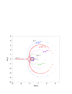
Figure 6: Complex-$u$ zeros of the Ising model partition function on sections of the square lattice for $\mu=e^{i\theta}$ with $\theta=\pi/4$, $\pi/2$, $3\pi/4$, and $11\pi/12$. See text for details of calculation. The exact phase boundaries for $\theta=0$ and $\theta=\pi$ are also shown.

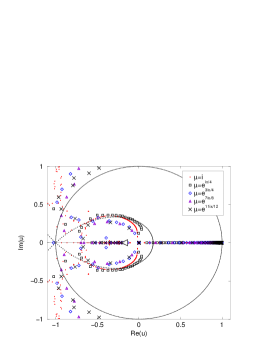
Figure 7: A closer view of the complex-$u$ partition function zeros in the region near $u=0$ for several values of $\theta$ in the range $0<\theta<\pi$. For reference the figure also shows, as exact results, the inner part of the curve forming the limaçon (77) for $\theta=0$ and the unit circle on ${\cal B}_{u}$ for $\theta=\pi$. For visual clarity, for $\theta=\pi$, we show only the right-hand endpoint, $u=-(3-2\sqrt{2})$, of the real line segment on ${\cal B}_{u}$ (indicated with the symbol $\lhd$). The lattice size is $12\times 13$ except for $\theta=\pi/2$, for which we show results with $L_{x}$ and $L_{y}$ up to 16.

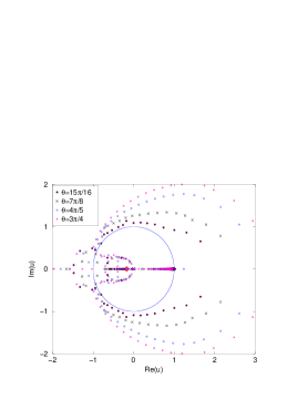
Figure 8: A closer view of the complex-$u$ partition function zeros in the inner central region for a several values of $\theta$ in the range $\pi/2<\theta<\pi$. Lattice size is $12\times 13$, as in Fig. 6.

Figure 9: Complex-$u$ zeros of the Ising model partition function with $\mu=e^{i\pi/2}=i$ on $L_{x}\times L_{y}$ sections of the square lattice with aspect ratio $\sim 1$ and $L_{x}$ and $L_{y}$ varying from 12 to 16.

As $\theta$ increases from zero, we observe a number of interesting features of the complex-$u$ zeros of the partition function. One important general feature is that for $\theta\neq 0$ mod $\pi$, zeros occur on the real axis, extending over an interval from the point where the inner loop of ${\cal B}_{u}$ is inferred to cross this axis, to a right-hand endpoint $u_{rhe}$ that increases as $\theta$ increases in the interval $0<\theta<\pi$. We infer that in the thermodynamic limit (i) these zeros merge to form a real line segment on ${\cal B}_{u}$ and (ii) the right-hand endpoint

$$u_{rhe}=e^{-4K_{rhe}}\equiv e^{-4J/(k_{B}T_{rhe})}$$ (81)

corresponds to the temperature $T_{rhe}$ at which the circular arc comprising ${\cal B}_{\mu}$ has endpoints at $\mu=e^{\pm i\theta}$. For infinite temperature, $K_{rhe}=0$, this endpoint (the Yang-Lee edge) occurs at $\theta=\pi$ and as the temperature decreases, the endpoints of the circular arc on ${\cal B}_{\mu}$ moves around to progressively smaller values of $\theta$. As $T$ decreases to the critical temperature $T_{c}=T_{PM-FM}$ for the onset of ferromagnetic long-range order, $\theta\to 0$, ${\cal B}_{\mu}$ closes to form the unit circle $|\mu|=1$, and for lower temperatures it remains closed. The property that $u_{rhe}$ and the corresponding temperature $T_{rhe}$ increase monotonically with $\theta$ in the range $0<\theta<\pi$ is equivalent to the property that the complex-conjugate endpoints of the circular arc comprising ${\cal B}_{\mu}$ (i.e., the Yang-Lee edge) at $\theta$ increases monotonically from $\theta=0$ at $T=T_{c}$ to $\theta\to\pi$ as $T\to\infty$. This thus establishes a 1–1 correspondence between the right-hand endpoint $u_{rhe}$ of the real line segment for a given $\theta$ and the temperature at which this $\theta$ is the value of the endpoint of the circular arc on ${\cal B}_{\mu}$. The limit $\theta\to 0$ involves special behavior, in that this real line segment shrinks to zero and disappears. The limit $\theta\to\pi$ is also special; again, the line segment on the positive real $u$ axis disappears in this limit and is replaced by a single zero at $u=1$ with multiplicity $n/2$, where $n$ denotes the number of sites on the lattice. This zero at $u=1$ gives rise to the term $(1/2)\ln(u-1)$ in the reduced free energy at $\mu=-1$ yl ; mw67 ; ih .

Turning on a finite (uniform) magnetic field, whether real or complex, does not remove the PM-AFM phase transition that occurs for sufficiently large negative $K=\beta J$. It follows that the outer loop on ${\cal B}_{u}$ cannot break. As discussed in only , this can be shown via a proof by contradiction. Assume that this outer loop on ${\cal B}_{u}$ did break; then one could analytically continue from the region around $K=0$, i.e., $u=1$, where the staggered magnetization $M_{st}$ vanishes identically, to the physical AFM phase where $M_{st}$ is nonzero, and similarly to the complex-$u$ extension of this AFM phase, which would be a contradiction. We find that as $\theta$ increases from 0 to $\pi$, the zeros that form the outer loop of ${\cal B}_{u}$ in the ${\rm Re}(u)>0$ half-plane move monotonically inward toward the unit circle $|u|=1$, which they form for $\theta\to\pi$. We infer that in the thermodynamic limit, (i) the right-most crossing on ${\cal B}_{u}$ decreases monotonically from $u=u_{PM-AFM}=(3+2\sqrt{2})\simeq 5.83$ to $u=1$ as $\theta$ increases from 0 to $\pi$; and (ii) the upper and lower points where the outer loop of ${\cal B}_{u}$ crosses the imaginary $u$ axis move monotonically inward from $u=\pm(2+\sqrt{3})i$ to $u=\pm i$. From inspection of the actual zeros that we calculate for various values of $\theta$, we infer the following approximate maximal values of $u$ at which ${\cal B}_{u}$ crosses the positive real $u$ axis: $u\simeq 5.5$ for $\theta=\pi/4$, $u\simeq 4.6$ for $\theta=\pi/2$, and $u\simeq 3.3$ for $\theta=3\pi/4$.

Recall that for nonzero real $h$, a theorem lp guarantees that the free energy for the ferromagnet is analytic for all temperatures, which means that ${\cal B}_{u}$ must break and retract from the real axis in the vicinity of what was, for $h=0$ the PM-FM phase transition point, $u_{PM-FM}$ lp . In contrast, the results of yl ; lp allow the free energy to be non-analytic as $H$ is varied at constant $\beta$ or $\beta$ is varied at constant $H$ (i.e., in both cases, as $h$ is varied) if $Re(h)=0$, that is, $h$ is pure imaginary, which is the situation that we consider here. Our most detailed study of the partition function zeros, for $\mu=i$ (see Fig. 9) is consistent with the conclusion that the inner loop on ${\cal B}_{u}$ does not break but remains closed. This conclusion is also consistent with our results for other values of $\theta$. In making this statement, we note that the fact that the zeros on the right-hand side of the inner loop, calculated on finite lattices, do not extend all the way in to the real axis, does not constitute evidence of a break in this loop in the thermodynamic limit. For example, even for the exactly solved case $\mu=1$, the zeros calculated on finite lattices also do not extend all of the way down to the real axis. In this context, we also remark on our exact results for quasi-1D strips; on both the toroidal and cyclic ladder strips, for $\mu=e^{i\theta}$, as $\theta$ is increased from 0 to $\pi$, the loop on ${\cal B}_{u}$ that passes through the critical point (at $u=0$) remains intact and unbroken. (Note that the point at which this loop crosses the real axis for these quasi-1D infinite-length ladder strips remains at $u=0$ as $\theta$ increases from 0 to $\pi$, while for the model in 2D the inferred crossing point of the inner loop moves gradually to the left as $\theta$ increases through this range for the square lattice.)

The details of the pattern of zeros in the complex-$u$ region that includes the real interval $-1\leq u\leq 0$ are complicated, and there is significant scatter of some of these zeros. Consequently, we do not try to make further inferences about the form of the complex-$u$ boundary ${\cal B}_{u}$ in this region in the thermodynamic limit. As an example of the kind of feature that might be present in this limit, one can discern some indication of possible triple points at $u\simeq-0.7\pm 0.2i$ and $u\simeq-0.9\pm 0.5i$. A complex-conjugate pair of triple points is, indeed, present in our exact solution for ${\cal B}_{u}$ on the toroidal ladder strip with $\mu=i$, as shown in Fig. 5. The scatter of zeros in this region raises the question of whether some part of ${\cal B}_{u}$ might actually fill out 2-dimensional areas rather than being one-dimensional (comprised of curves and possible line segments) in the thermodynamic limit. For the 2D Ising model in zero field it is easy to see that complex-$u$ zeros generically fill out areas if the spin-spin exchange constants in the $x$ and $y$ directions are unequal, but this is not directly relevant here, since we only consider the model with isotropic couplings. For isotropic couplings, this area behavior happens for a heteropolygonal Archimedean lattice, namely the $4\cdot 8\cdot 8$ lattice cmo , and here again, the origin of this is obvious from the exact form of the free energy (see eq. (6.5) and Fig. 7 of cmo ). One can fit curves or line segments to many of the zeros in Fig. 6. As for the region where the zeros show scatter, our results are not conclusive, and we do not try to make any inference about whether or not some set of these zeros might merge to form areas in the thermodynamic limit.

Several other aspects of the real zeros are of interest. First, we find that as $\theta$ increases from 0, there are real zeros not just to the right of the extrapolated point where the inner loop on ${\cal B}_{u}$ crosses the real axis, but also to the left of this point. Indeed, we find that for $0<\theta\leq\pi$, there are zeros on the negative real axis. As $\theta\to\pi$, these occur in the interval of eq. (80), i.e., $-(3+2\sqrt{2})\leq u\leq-(3-2\sqrt{2})$. On the finite lattices that we have studied, we also have found complex-conjugate pairs of zeros that are close to the zeros on the real axis.

The value $\theta=\pi/2$, i.e., $\mu=i$, is the middle of the range under consideration here, and we have devoted a particularly intensive study to it. In addition to the general plots comparing the zeros for this value of $\theta$ with those for other values of $\theta$, we show the zeros for this case alone in Fig. 9. The zeros shown in this figure were calculated for several different lattice sizes with aspect ratio $L_{y}/L_{x}\simeq 1$ and $L_{x}$ ranging from 12 to 16. We display the zeros for different lattice sizes together to see lattice size-dependent effects. As is evident from the figure, much of the locus comprised by these zeros is largely independent of lattice size for sizes this great. These calculations illustrate our general description of the properties of ${\cal B}_{u}$ above. From these zeros we infer that for $\mu=i$, in the thermodynamic limit, (i) the complex-$u$ phase boundary ${\cal B}_{u}$ crosses the real axis at $u\simeq 4.6$ and the imaginary axis at $u\simeq\pm 2.7i$; (ii) there is an inner loop on ${\cal B}_{u}$ which is likely to pass through $u=0$, although there is some decrease in the density of complex zeros in the vicinity of this point; (iii) the locus ${\cal B}_{u}$ exhibits a line segment on the real axis that extends from a right-hand endpoint $u_{rhe}\simeq 0.8$ leftward with components along the negative real axis; and although the details of this line segment at intermediate points cannot be inferred with certitude, the left-most endpoint occurs at $u_{\ell he}\simeq-4.5$; (v) the phase boundary ${\cal B}_{u}$ thus appears to separate the $u$ plane into at least four regions: (a) the AFM phase and its complex-$u$ extension, which occupies values of $u$ going outward to complex infinity, (b) the interior of the outer loop; (c) and the complex-conjugate pair of regions inside of the inner loop, which seems to be divided into an upper and lower part by the real line segment inside this loop. As regards item (i), the points at which the outer loop of ${\cal B}_{u}$ crosses the imaginary $u$ axis are consistent, to within the accuracy of our calculations, with being equal to $\pm(1+\sqrt{3})i$.

VII.2 Connections with Results on Quasi-1D Strips for $\mu=e^{i\theta}$

With appropriate changes to take account of the change in dimensionality, we can relate these features to our exact results on quasi-1D strips. For these strips we found that the locus ${\cal B}_{u}$ includes a line segment on the positive real axis in the physical ferromagnetic interval as $\theta$ increases above zero. In the 1D case, we found the simple result $u_{rhe}=\sin^{2}(\theta/2)$ in eq. (17) for the right-hand endpoint of this line segment. For the toroidal and cyclic ladder strips we illustrated, e.g. for $\theta=\pi/2$ ($\mu=i$), how it is determined as the root of the respective polynomials, eqs. (69) and (73), that occur in the solution of a relevant cubic equation for the eigenvalue of the transfer matrix. In Table 1 we showed the values of $u_{rhe}$ for the 1D line and the toroidal strip, together with the corresponding values of the temperature $T_{rhe}$, as a function of $\theta\equiv\theta_{e}$. This table shows how $u_{rhe}$ and $T_{rhe}$ increase as $\theta$ increases above 0 and approaches $\pi$. We also noted how, for a given value of $\theta$, $T_{rhe}$ increases as one increases the strip width. This is physically understandable, since a given value of the angle $\theta$ corresponds to a higher temperature and hence larger $u_{rhe}$ as the strip width increases because that increase fosters short-range ferromagnetic ordering.

Another property of the zeros that can be related to our exact results on quasi-1D strips is the part of the line segment extending to the left of the point where the inner loop appears to cross the real axis and, indeed, extending to negative real values. For the quasi-1D strips, these intervals are the same, since the ferromagnetic critical point is at $u=0$. For the 1D line case, the locus ${\cal B}_{u}$, which is $u\leq\sin^{2}(\theta/2)$, includes the semi-infinite line segment $u<0$. For the toroidal ladder strip, we find that for any $\theta$ in the interval $0<\theta<\pi$, ${\cal B}_{u}$ includes the segment $-1\leq u\leq 0$ as well as the portion on the positive real axis discussed above. So there are again similarities with respect to this feature as regards the results for the strips and for our zeros calculated on patches of the square lattice. In future work it would be of interest to calculate complex-$u$ zeros of the Ising model partition function with imaginary $h$ on $d=3$ lattices, as was done for real $h$ in Ref. ipz .

VIII Connection of Singular Behavior of the Zero Density in the $\mu$ and $u$ Planes

For the ferromagnetic Ising model, studies have been carried out of the singularity at the endpoint of the circular arc ${\cal B}_{\mu}$ as $\theta\to\theta_{e}$ (Yang-Lee edge) and the associated density of zeros $g(\theta)$ in the original papers yl and in works including those by Griffiths, Fisher and collaborators, and Cardy kg -cardy85 . Kim has suggested that the singularity at an edge of a locus of zeros in the $u$ plane is equivalent to the Yang-Lee edge singularity kim3d . For the case of $d=2$ dimensions, we can show this equivalence using conformal field theory methods. We recall that for a conformal field theory indexed by (relatively prime) positive integers $p$ and $p^{\prime}$, the central charge $c$ is

$$c=1-6\frac{(p-p^{\prime})^{2}}{pp^{\prime}}$$ (82)

with scaling dimensions

$$h_{r,s}=\frac{[(pr-p^{\prime}s)^{2}-(p-p^{\prime})^{2}]}{4pp^{\prime}}\ ,$$ (83)

where $1\leq r\leq p-1$ and $1\leq s\leq p^{\prime}-1$. The requirement of a single scaling field (other than the identity) leads uniquely to the identification of the conformal field theory as ${\cal M}_{5,2}$, which is non-unitary, with central charge $c=-22/5$ cardy85 . The scaling dimension for the single non-identity field is $\eta=4h_{1,2}=-4/5$. From this and the standard relation $\eta=d+2-2y_{h}$, where $y_{h}$ is the magnetic exponent, it follows that $y_{h}=12/5$. Since the theory has only one relevant scaling field, the thermal exponent is the same, i.e.

$$y_{t}=y_{h}=\frac{12}{5}\ .$$ (84)

Substituting the value of $\eta$ into the scaling relation (32) with $d=2$ yields the result $\sigma=-1/6$ fisher78 ; cardy85 . The equal thermal and magnetic exponents in eq. (84) determine all of the rest of the exponents for this critical point, which include

$$\nu_{e}^{\prime}=\frac{1}{y_{t}}=\frac{5}{12}$$ (85)

$$\alpha_{e}^{\prime}=2-\frac{d}{y_{t}}=\frac{7}{6}$$ (86)

$$\beta_{e}=\frac{d-y_{h}}{y_{t}}=-\frac{1}{6}$$ (87)

$$\gamma_{e}^{\prime}=\frac{2y_{h}-d}{y_{t}}=\frac{7}{6}\ .$$ (88)

(These results have also been independently and simultaneously obtained in this manner by B. McCoy.) The fact that the conformal field theory has only a single non-identity operator and equal thermal and magnetic exponents leads to the conclusion that the exponent $1-\alpha_{e}^{\prime}$ describing the singular behavior of the density of zeros at the right-hand endpoint $u_{e}=u_{rhe}$ of the positive real line segment on ${\cal B}_{u}$ corresponding to a value of $\theta$ with $\mu=e^{i\theta}$, $0<\theta<\pi$, is the same as the exponent $\sigma$ describing the singular behavior of the density of zeros at the complex-conjugate endpoints of the circular arcs on ${\cal B}_{\mu}$.

A parenthetical remark may be of interest here. We recall that a liquid-gas phase transition may be modelled as a lattice gas, and the latter may, in turn, be mapped onto a ferromagnetic Ising model. In this context the Yang-Lee circle theorem states that the zeros of the partition function occur on the unit circle $|z|=1$ in the complex plane of the fugacity, $z=e^{\beta\mu^{\prime}}$ (where $\mu^{\prime}$ is the chemical potential) and, in the thermodynamic limit, form an arc of this unit circle extending from $\theta=\pi$ over to complex-conjugate endpoints at $z=e^{\pm i\theta_{e}}$ yl . For closed-form approximations to the equation of state of a liquid-gas system such as that of van der Waals, the density of Yang-Lee zeros has been calculated ky ; hh . For intermolecular potentials with a repulsive hard core, the expansion of the reduced pressure $pv_{0}/(k_{B}T)$ in powers of fugacity, $pv_{0}/(k_{B}T)=\sum_{j=1}^{\infty}b_{\ell}z^{\ell}$, exhibits alternating signs, indicating a singularity on the negative real $z$ axis groen . This latter singularity has been shown to be equivalent to the Yang-Lee edge singularity lf ; pf . This is a somewhat different equivalence than the one discussed here, since it relates the Yang-Lee singularities at $z=e^{\pm i\theta_{e}}$ to one on the negative real $z$ axis, whereas the relation discussed here is between the Yang-Lee singularities and a singularity on the (positive) real $u$ axis.

Now consider a switch from the imaginary values of $h$ relevant for the Yang-Lee edge singularity to real values of $h$. These lead to the complex-conjugate arcs on ${\cal B}_{u}$ with arc (prong) endpoints $u_{e}$ and $u_{e}^{*}$ that retract from the position of what was the critical point at $u=u_{c}$ (for $h=0$) as $|h|$ increases from zero only . Again, the fact that the conformal field theory has only a single non-identity operator and equal thermal and magnetic exponents leads us to the further conclusion that the exponent $1-\alpha_{e}^{\prime}$ describing the singular behavior of the zeros at the ends of the complex-conjugate arcs in the complex $u$ plane at $u_{e}$ and $u_{e}^{*}$ (cf. eq. (23) with $u_{s}=u_{e}$) is the same as the exponent $\sigma$. With $\alpha_{e}^{\prime}=7/6$, this implies that for the 2D Ising model, $g(u)$ thus diverges at these arc endpoints with the exponent

$$1-\alpha_{e}^{\prime}=\sigma=-\frac{1}{6}\quad(2D),$$ (89)

We also conclude that the exact values of the exponents $\alpha_{e}^{\prime}$, $\beta_{e}$, and $\gamma_{e}^{\prime}$ for the specific heat, magnetization, and susceptibility in eqs. (86)-(88) apply to the arc endpoints at $u_{e}$ and $u_{e}^{*}$. These exact values agree very well with the numerical values that we obtained in only from our analysis of low-temperature, high-field (i.e., small-$u$, small-$\mu$) series (see Table I of only ). These values had been suggested in kim3d based on the assumption that $y_{t}=y_{h}=12/5$ for the endpoint of a locus of zeros in the $u$ plane. Here we have proved the equivalence using conformal field theory methods.

In only we also studied complex values of $h$ corresponding to negative $\mu$ in the real interval $-1<\mu<0$. For the solvable case $\mu=-1$ one knows the exponents $\alpha^{\prime}_{s}$ and $\beta_{s}$ exactly at various singular points, and in ih , from analyses of series, we obtained the exponent $\gamma^{\prime}_{s}$ and inferred exact values for this exponent also. These singular points at $\mu=-1$ include the multiple point $u=-1$, the left- and right-hand endpoints of the line segment $u_{\ell he}=-(3+2\sqrt{2})$ and $u_{rhe}=1/u_{\ell he}=-(3-2\sqrt{2})$, and also the point $u=1$. For reference, in ih we obtained $\alpha_{e}^{\prime}=1$, $\beta_{e}=-1/8$, and $\gamma_{e}^{\prime}=5/4$ at $u_{e}=-(3-2\sqrt{2})$, $\alpha_{s}^{\prime}=0$ ($C_{H}$ finite), $\beta_{s}=1/2$, and $\gamma_{s}^{\prime}=1$ at $u=-1$, and $\alpha_{s}^{\prime}=0$ ($C_{H}$ finite), $\beta_{s}=-1/4$, and $\gamma_{s}^{\prime}=5/2$ at $u=1$ (see Table 4 of that paper), where the results for $\alpha^{\prime}$ and $\beta$ were exact and the results for $\gamma^{\prime}$ were inferred from our analysis of series. (Exponents at $u_{rhe}=1/u_{\ell he}$ are related by the $u\to 1/u$ symmetry.) For $\mu$ close, but not equal, to $\mu=-1$, the line segment on the negative real axis shifted slightly, and there appeared a new line segment on the positive real axis extending inward from the right-most portion of the boundary ${\cal B}_{u}$. We also studied these singular exponents via series analyses in only . In future work it would be worthwhile to understand better the values of the exponents describing these singularities for negative real $\mu$.

IX Conclusions

In this paper we have studied properties of the Ising model in the complex $u$ plane for nonzero magnetic field. We used exact results for infinite-length quasi-1D strips to provide insights into the previous results that we had obtained in ih ; only . We also studied the case of complex $h$, in particular, the case of imaginary $h$, for which $\mu=e^{i\theta}$. We used both exact results on strips and partition function zeros to analyze the phase diagram in the $u$ plane for this range of $\mu$. One important result that we found was that the boundary ${\cal B}_{u}$ contains a real line segment extending through part of the physical ferromagnetic interval $0\leq u\leq 1$, with a right-hand endpoint $u_{rhe}$ at the temperature for which the Yang-Lee edge singularity occurs at $\mu=e^{\pm i\theta}$. We also used conformal field theory arguments to relate the singularities at $u_{rhe}$ and the Yang-Lee edge.

- (1) L. Onsager, Phys. Rev. 65, 117 (1944).
- (2) C. N. Yang, Phys. Rev. 85, 808 (1952).
- (3) B. McCoy and T. T. Wu, The Two-Dimensional Ising Model (Harvard University Press, Cambridge, 1968).
- (4) C. N. Yang and T. D. Lee, Phys. Rev. 87, 404 (1952); T. D. Lee and C. N. Yang, Phys. Rev. 87, 410 (1952).
- (5) M. E. Fisher, Lectures in Theoretical Physics (Univ. of Colorado Press, Boulder, 1965), vol. 7C, p. 1.
- (6) C. Domb and A. J. Guttmann, J. Phys. C 3, 1652 (1970).
- (7) B. M. McCoy and T. T. Wu, Phys. Rev. 155, 438 (1967).
- (8) K. Y. Lin and F. Y. Wu, Int. J. Mod. Phys. B 4, 471 (1988).
- (9) V. Matveev and R. Shrock, J. Phys. A 28, 4859 (1995).
- (10) V. Matveev and R. Shrock, Phys. Rev. E 53, 254-267 (1996).
- (11) V. Matveev and R. Shrock, Phys. Lett. A 215, 271 (1996).
- (12) M. F. Sykes, D. S. Gaunt, J. L. Martin, S. R. Mattingly, and J. W. Essam, J. Math. Phys. 14, 1071 (1973); M. F. Sykes, M. G. Watts, and D. S. Gaunt, J. Phys. A 8, 1448 (1975).
- (13) R. J. Baxter and I. G. Enting, J. Stat. Phys. 21, 103 (1979).
- (14) S.-Y. Kim, Phys. Rev. E 71, 017102 (2005).
- (15) I. Jensen, J.-M. Maillard, V. Matveev, B. M. McCoy, and R. Shrock, work in progress, to appear.
- (16) R. Shrock, Physica A 283, 388 (2000).
- (17) S.-C. Chang and R. Shrock, Physica A 286, 189 (2000).
- (18) S.-C. Chang and R. Shrock, Physica A 296, 183 (2001).
- (19) R. Abe, Prog. Theor. Phys. 37, 1070 (1967); Prog. Theor. Phys. 38, 322 (1967).
- (20) V. Matveev and R. Shrock, J. Phys. A 28, 1557 (1995).
- (21) O. Stormark and C. Blomberg, Physica Scripta 1, 47 (1970).
- (22) C. Blomberg, Physica Scripta 2, 117 (1970).
- (23) M. Suzuki, Prog. Theor. Phys. 38, 1225 (1967).
- (24) Z. Glumac and K. Uzelac, J. Phys. A 27, 7709 (1994).
- (25) J. L. Lebowitz and O. Penrose, Commun. Math. Phys. 11, 99 (1968).
- (26) H. J. Brascamp and H. Kunz, J. Math. Phys. 15, 65 (1974).
- (27) D. A. Bini and G. Fiorentino, Numerical Algorithms 23, 127 (2000); MPSolve program available at http://www.dm.unipi.it/cluster-pages/mpsolve/index.htm .
- (28) V. Matveev and R. Shrock, J. Phys. A 28, 5235 (1995).
- (29) C. Itzykson, R. B. Pearson and J.-B. Zuber, Nucl. Phys. B 220, 415 (1983).
- (30) P.J. Kortman and R.B. Griffiths, Phys. Rev. Lett. 27, 1439 (1971).
- (31) D.A. Kurtze and M.E. Fisher, Phys. Rev. B 20, 2785 (1979).
- (32) M. E. Fisher, Phys. Rev. Lett. 40, 1610 (1978).
- (33) J. L. Cardy, Phys. Rev. Lett.. 54, 1354-1356 (1985).
- (34) S.-Y. Kim, Nucl. Phys. B 637, 409 (2002).
- (35) S. Katsura, J. Chem. Phys. 22, 1277 (1954).
- (36) J. Groeneveld, Phys. Lett. 3, 50 (1962).
- (37) P. C. Hemmer and E. Hiis Hauge, Phys. Rev. 133, A1010 (1964).
- (38) S.-N. Lai and M. E. Fisher, J. Chem. Phys. 103, 8144 (1995).
- (39) Y. Park and M. E. Fisher, Phys. Rev. E 60, 6323 (1999).