Superfluid and Mott Insulator phases of one-dimensional Bose-Fermi mixtures

Abstract

We study the ground state phases of Bose-Fermi mixtures in one-dimensional optical lattices with quantum Monte Carlo simulations using the Canonical Worm algorithm. Depending on the filling of bosons and fermions, and the on-site intra- and inter-species interaction, different kinds of incompressible and superfluid phases appear. On the compressible side, correlations between bosons and fermions can lead to a distinctive behavior of the bosonic superfluid density and the fermionic stiffness, as well as of the equal-time Green functions, which allow one to identify regions where the two species exhibit anticorrelated flow. We present here complete phase diagrams for these systems at different fillings and as a function of the interaction parameters.

I Introduction

The experimental realization of strongly correlated systems with ultracold gases loaded in optical lattices greiner02 has generated tremendous excitement during recent years. Initially thought of as a way to simulate condensed matter model Hamiltonians, like the Bose-Hubbard Hamiltonian jaksch98 , loading atoms on optical lattices has enabled the creation of quantum systems that are unexpected in the condensed matter context. Among these systems the realization of Bose-Fermi mixtures in optical lattices ott04 ; gunter06 ; ospelkaus06 , where the inter- and intra-species interactions can be tuned to be attractive or repulsive zaccanti06 , is a remarkable example of the scope of realizable models.

Theoretical studies of Bose-Fermi mixtures in one-dimensional lattices have been done for homogeneous cazalilla03 ; lewenstein04 ; mathey04 ; imambekov06 ; pollet06 ; sengupta07 ; hebert07 ; mering08 and trapped albus03 ; cramer04 ; pollet06a systems. Several approaches have been used: Gutzwiller mean-field theory albus03 , strong coupling expansions lewenstein04 ; mering08 , bosonization cazalilla03 ; mathey04 and exact analytical imambekov06 and numerical pollet06 ; sengupta07 ; hebert07 ; pollet06a ; mering08 studies. Recently, a mixture of bosonic atoms and molecules on a lattice was studied numerically rousseau01 . The landscape of phases encountered is expansive, and includes Mott insulators, spin and charge density waves, a variety of superfluids, phase separation, and Wigner crystals. However, the phase diagram in the chemical potential-interaction strength plane has not yet been reported.

It is our goal in this paper to present a study of repulsive Bose-Fermi mixtures in one-dimensional lattices that generalizes previous studies, which focused on specific special densities, to more general filling. After mapping the phase diagram we will explore different sections in greater detail. Since the particular case in which the lattice is half filled with bosons and half filled with fermions has been carefully studied in Ref. pollet06 , we will instead concentrate here on two cases: (i) when the number of bosons is commensurate with the lattice size but the number of fermions is not, and (ii) when the sum of both species is commensurate with the lattice size but the number of bosons and fermions are different. Some of the phases present in these cases have been identified by Sengupta and Pryadko in their grand canonical study in Ref. sengupta07 and by Hébert et al. in the canonical study recently presented in Ref. hebert07 .

The Hamiltonian of Bose-Fermi mixtures in one dimension can be written as

$$\hat{H}= - t_{B}\sum_{l}(\,b^{\dagger}_{l+1}b^{\phantom{\dagger}}_{l}+b^{\dagger}_{l}b^{\phantom{\dagger}}_{l+1}\,)$$ (1)

$$- t_{F}\sum_{l}(\,f^{\dagger}_{l+1}f^{\phantom{\dagger}}_{l}+f^{\dagger}_{l}f^{\phantom{\dagger}}_{l+1}\,)$$

$$+ U_{BB}\sum_{l}\,\hat{n}^{B}_{l}(\hat{n}^{B}_{l}-1)+U_{BF}\sum_{l}\,\hat{n}^{B}_{l}\hat{n}^{F}_{l}$$

where $b_{l}^{\dagger}(b^{\phantom{\dagger}}_{l})$ are the boson creation (destruction) operators on site $l$ of the one-dimensional lattice with $L$ sites. Similarly, $f_{l}^{\dagger}(f^{\phantom{\dagger}}_{l})$ are the creation (destruction) operators on site $l$ for spinless fermions on the same lattice. For these creation and destruction operators $\hat{n}^{B,F}_{l}$ are the associated number operators. The bosonic and fermionic hopping parameters are denoted by $t_{B}$ and $t_{F}$ respectively, and the on-site boson-boson and boson-fermion interactions by $U_{BB}$ and $U_{BF}$. In this paper we will consider the case $t_{B}=t_{F}=1$ (i.e. when the boson and fermion hopping integrals are equal) and choose $t_{B}=1$ to set the scale of energy.

It is useful to begin a discussion of the phase diagram with an analysis of the zero hopping limit ($t_{B}=t_{F}=0$) similar to the one done by Fisher et al. in Ref. fisher89 for the purely bosonic case. Consider a particular fermion occupation of one fourth of the lattice sites, $N_{F}=L/4$ fixed. Bosons can be added up to $N_{B}=3L/4$ without sitting on a site which is already occupied by either a boson or a fermion. Therefore the associated chemical potential $\mu$ is small. What happens when $N_{B}$ exceeds $3L/4$ depends on the relative strength of $U_{BB}$ and $U_{BF}$.

If $U_{BF}$ is less than $2U_{BB}$ then the extra bosons sit atop of the fermions and $\mu$ jumps by $U_{BF}$. The chemical potential stays at this elevated value of $U_{BF}$ until all the sites with fermions also have a boson. At that point additional bosons start going onto sites with a boson already, and $\mu$ jumps to $2U_{BB}$. Thus in general there are incompressible phases where the boson chemical potential jumps both at commensurate $\rho_{B}=1,\,2,\,3,...$ (as for the pure boson-Hubbard model) and also at $\rho_{B}=1-\rho_{F},\,\,2-\rho_{F},\,\,3-\rho_{F},\cdots$. For $U_{BF}$ greater than $2U_{BB}$ and less than $6U_{BB}$ the incompressible phases still start at $\rho_{B}=1-\rho_{F}$ but the following potential jumps are shifted up by $1-\rho_{F}$. Turning on the hoppings $t_{B},t_{F}$ introduces quantum fluctuations which will ultimately destroy these Mott plateaus and introduce new, intricate phases.

II Canonical Worm Algorithm

We perform Quantum Monte Carlo simulations (QMC) using a recently proposed Canonical Worm algorithm vanhoucke06 ; rombouts06 . This approach makes use of global moves to update the configurations, samples the winding number, and gives access to the measurement of $n$-body Green functions. It also has the useful property of working in the canonical ensemble. This is particularly important for the present application since working with two species of particles leads to two different chemical potentials in the grand canonical ensemble. These prove difficult to adjust such that the precise, desired fillings are achieved. In our canonical simulations the Bose and Fermi occupations are exactly specified and the chemical potentials $\mu_{B}$ and $\mu_{F}$ are instead computed batrouni90 via appropriate numerical derivatives of the resultant ground state energy (e.g. $\mu_{B}=E_{0}(N_{B}+1)-E_{0}(N_{B})$).

The Canonical Worm algorithm is a variation of the Prokof’ev et al. grand-canonical worm algorithm prokofev98 . Within the Canonical Worm approach one starts by writing the Hamiltonian as $\hat{H}=\hat{V}-\hat{T}$, where $\hat{T}$ is comprised of the non-diagonal terms and is by necessity positive definite. The partition function $\mathcal{Z}=\textrm{Tr}e^{-\beta\hat{H}}$ takes the form

$$\mathcal{Z} = \textrm{Tr }e^{-\beta\hat{V}}\textbf{T}_{\tau}e^{\int_{0}^{\beta}\hat{T}(\tau)d\tau}$$ (2)

$$= \textrm{Tr }e^{-\beta\hat{V}}\sum_{n}\int_{0<\tau_{1}<\cdots<\tau_{n}<\beta}\!\!\!\!\!\!\!\!\!\!\!\!\!\!\!\!\!\!\!\!\!\!\!\!\!\!\!\!\!\!\!\!\hat{T}(\tau_{n})\cdots\hat{T}(\tau_{1})d\tau_{1}\cdots d\tau_{n}$$ (3)

where $\hat{T}(\tau)=e^{\tau\hat{V}}\hat{T}e^{-\tau\hat{V}}$. In order to sample expression (3) an extended partition function is considered by breaking up the propagator at imaginary time $\tau$ and introducing a “worm operator” $\hat{W}=\sum_{ijkl}w_{ijkl}b_{i}^{\dagger}b^{\phantom{\dagger}}_{j}f_{k}^{\dagger}f^{\phantom{\dagger}}_{l}$ that leads to $\mathcal{Z}(\tau)=\textrm{Tr}e^{-(\beta-\tau)\hat{H}}\hat{W}e^{-\tau\hat{H}}$. Complete sets of states are introduced between consecutive $\hat{T}$ operators to allow a mapping of the 1D quantum problem onto a 2D classical problem where a standard Monte Carlo technique can be applied. Measurements can be performed when configurations resulting in diagonal matrix elements of $\hat{W}$ occur. This way unphysical movements are exploited to help explore the Hilbert space, but are ignored when sampling for measurements.

As with pure bosonic systems, the evolution of the boson and fermion densities $\rho_{B},\rho_{F}$ with the associated chemical potential $\mu_{B},\mu_{F}$ identifies Mott insulating behavior fisher89 . A jump in $\mu$ signals a Mott phase where the compressibility $\kappa_{B}=\partial\rho_{B}/\partial\mu_{B}$ or $\kappa_{F}=\partial\rho_{F}/\partial\mu_{F}$ vanishes.

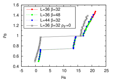
Figure 1: (Color online) $\rho_{B}$ as a function of chemical potential $\mu_{B}$. The fermion density is $\rho_{F}=1/4$ and the interaction strengths are fixed at $U_{BB}=10$ and $U_{BF}=16$. There are Mott plateaus at $\rho_{B}=1-\rho_{F}=3/4$ and $\rho_{B}=1$ as predicted by the $t_{B}=t_{F}=0$ analysis. The positions of the Mott lobes coincide for different lattice sizes $L=36,44$ and temperatures $\beta=32,48$ to within our error bars, which are smaller than the symbol size. The dependence of $\rho_{B}$ on $\mu_{B}$ in the absence of fermions is given for comparison.

Quantities of interest that we measure include the bosonic superfluid density and the fermionic stiffness,

$$\rho^{\rm s}_{B} = \big{\langle}W_{B}^{2}\big{\rangle}L/2\beta$$

$$\rho^{\rm s}_{F} = \big{\langle}W_{F}^{2}\big{\rangle}L/2\beta\,\,.$$ (4)

Here $\langle W^{2}\rangle$ are the associated winding numbers. Correlations between the bosonic and fermionic winding numbers pollet06 are determined by the combinations,

$$\rho^{\rm s}_{c} = \big{\langle}(W_{B}+W_{F})^{2}\big{\rangle}L/2\beta$$

$$\rho^{\rm s}_{a} = \big{\langle}(W_{B}-W_{F})^{2}\big{\rangle}L/2\beta\,\,.$$ (5)

In addition to the usual bosonic and fermionic Green function,

$$G_{ij}^{B} = \big{\langle}b_{i}^{\dagger}b^{\phantom{\dagger}}_{j}\big{\rangle}$$

$$G_{ij}^{F} = \big{\langle}f_{i}^{\dagger}f^{\phantom{\dagger}}_{j}\big{\rangle}\,\,,$$ (6)

we also measure the composite anti-correlated two-body Green function

$$G_{ij}^{a} = \big{\langle}b_{i}^{\dagger}b^{\phantom{\dagger}}_{j}f_{j}^{\dagger}f^{\phantom{\dagger}}_{i}\big{\rangle}\,\,.$$ (7)

In $G_{ij}^{a}$, the fermion and boson propagate in opposite directions (one from $j$ to $i$ and one from $i$ to $j$).

The Fourier transforms of $G^{B}_{ij}$ and $G^{F}_{ij}$ give the densities $n_{B}(k)$ and $n_{F}(k)$ in momentum space; $n_{a}(k)$ is the Fourier transform of the composite two-body Green function $G^{a}_{ij}$.

We performed extensive checks of the code against other quantum Monte Carlo simulations in the pure boson and pure fermion cases, and against exact diagonalization and Lanczos calculations for mixed systems on small lattices.

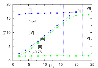
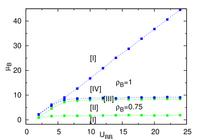
Figure 2: (Color online) Top panel: Phase diagram in the $\mu_{B}$-$U_{BF}$ plane for $U_{BB}=10$ and $\rho_{F}=1/4$ obtained by a sequence of plots such as that in Fig. 1. The vertical line at $U_{BF}=16$ corresponds to the coupling value in Fig. 1. Within the regions labeled $\rho_{B}=0.75$ and $\rho_{B}=1$, the boson density is frozen even though the chemical potential varies. The $\rho_{B}=1$ lobe is pinched off at $U_{BF}\approx 2U_{BB}$. The labeling of the phases is: I. Superfluid ($\rho^{\rm s}_{B}\neq 0$ $\rho^{\rm s}_{F}\neq 0$); II. Anti-Correlated phase ($\rho^{\rm s}_{B}\neq 0$, $\rho^{\rm s}_{F}\neq 0$, $\rho^{\rm s}_{B}=\rho^{\rm s}_{F}$); III. Anti-Correlated phase / Relay Superfluid ($\rho^{\rm s}_{B}\neq 0$, $\rho^{\rm s}_{F}\neq 0$) (see text for detailed explanation); IV. Mott Insulator / Luttinger liquid ($\rho^{\rm s}_{B}=0$, $\rho^{\rm s}_{F}\neq 0$); V. Insulator, $\rho^{\rm s}_{B}=0$ $\rho^{\rm s}_{F}=0$; VI. Phase separation.
Bottom panel: Phase diagram in the $\mu_{B}$-$U_{BB}$ plane for $U_{BF}=10$ and $\rho_{F}=1/4$. The upper boundary of phase $II$ is defined by the increase of energy when a boson is added at filling $\rho_{B}+\rho_{F}=1$; this is approximately $\mu_{B}=U_{BF}$ (for $U_{BF}<2U_{BB}$), a line of slope 1 in the $\mu_{B}$-$U_{BF}$ plane and slope 0 in the $\mu_{B}$-$U_{BB}$ plane. A similar strong coupling analysis applies for the other boundaries. (See also Fig. 13 and [lewenstein04, ].)

III Phase Diagram in the $\mu_{B}$-$U_{BF}$ plane

We begin our determination of the phase diagram by calculating the dependence of the density $\rho_{B}$ on chemical potential $\mu_{B}$, mapping out the extent that the Mott plateaus described in the introduction survive the introduction of quantum fluctuations $t_{B},t_{F}$. We examine a system with a fixed $U_{BB}=10$ and $\rho_{F}=1/4$ and focus on the regions through $\rho_{B}\leq 3/2$ and $U_{BF}\leq 5U_{BB}/2$ in the phase diagram. The $t_{B}=t_{F}=0$ analysis suggests for $U_{BF}<2U_{BB}$ there will be plateaus with compressibility $\kappa=0$ at $\rho_{B}+\rho_{F}=1$ (i.e. $\rho_{B}=3/4$) caused by $U_{BF}$ and at $\rho_{B}=1$ caused by $U_{BB}$. Fig. 1 exhibits these plateaus for $U_{BF}=16$ and $t_{B}=t_{F}=1$. The complete phase diagram in the $\mu_{B}$-$U_{BF}$ plane at fixed $U_{BB}=10$ is obtained by replicating Fig. 1 for different $U_{BF}$, and is given in Fig. 2a. For weak $U_{BF}$ the phase diagram is dominated by the $\rho_{B}=1$ plateau where the chemical potential jumps by $2U_{BB}-U_{BF}\approx 2U_{BB}=20$. As $U_{BF}$ increases, this plateau shrinks and finally terminates at $U_{BF}\approx 2U_{BB}=20$. At the same time, the plateau at $\rho_{B}=1-\rho_{F}$ grows to $U_{BF}=20$. The explanation of the labeling of the different phases (I-VI) will be given after we discuss the superfluid response of the system. Fig. 2b shows the phase diagram in the $\mu_{B}$ and $U_{BB}$ plane.

IV Superfluid Response at $\rho_{B}+\rho_{F}=1$

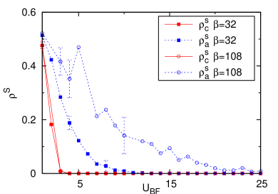
Figure 3: (Color online) “Horizontal” sweep, that is fixed densities $\rho_{B}=3/4$ and $\rho_{F}=1/4$ and varying $U_{BF}$, through the phase diagram of Fig. 2. As in Figs. 1 and 2, $U_{BB}=10$. Top panel: Both the bosonic and fermionic species exhibit a finite stiffness at weak coupling (region II of phase diagram), which decays as $U_{BF}$ increases until insulating behavior occurs (region V of phase diagram). Bottom panel: Near $U_{BF}=0$ both $\rho^{\rm s}_{c}\neq 0$ and $\rho^{\rm s}_{a}\neq 0$ are very similar. However, quickly after turning on $U_{BF}$, the correlated and anti-correlated stiffness show that the bosons and fermions propagate in opposite directions $\rho^{\rm s}_{a}\neq 0$, while $\rho^{\rm s}_{c}=0$.

After determining the positions of the Mott plateaus, we examine the stiffness and Green functions. We take a “horizontal” cut through Fig. 2a by fixing $\rho_{B}+\rho_{F}=1$ ($\rho_{B}=3/4$) and increasing $U_{BF}$. In Fig. 3 we see that for $U_{BF}\lesssim 2U_{BB}=20$ the interaction strength $U_{BF}$ is small enough that fermions and bosons can briefly inhabit the same site. Now, when a boson visits the site of a neighboring fermion (or vice versa) it is equally likely that the fermion will exchange as for the boson to return to its original site. Through these exchanges the bosons and fermions can achieve anti-correlated winding around the lattice. Thus, the bosonic superfluid density and the fermionic stiffness are both non-zero and identical . However, as $U_{BF}$ increases past $U_{BF}\approx 2U_{BB}=20$ the cost of double occupancy becomes prohibitive. With its benefits outweighed by energy penalties exacted by $U_{BF}$, all anti-correlated “superfluidity” ceases. Pollet et al. pollet06 have argued that this region exhibits phase separation. Indeed we do detect a signal of phase separation through density structure factor. But the signal is weak, about 20 times weaker than what we get at phase VI (next section), and compressibility is close to zero, so we label this region as an insulator.

From the results depicted in Fig. 3 one should notice that while for quantities like the energy and Mott gap $\beta=32$ is sufficiently low for $L=32$ to capture the ground state behavior, for stiffnesses one requires much lower temperatures.

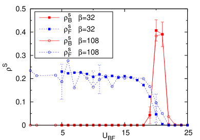
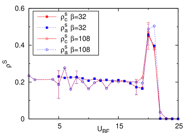
Figure 4: (Color online) Same “horizontal cut” as Fig. 3 except at commensurate density for the boson species alone $\rho_{B}=1$ and $\rho_{F}=1/4$. Top panel: The bosons are insulating at weak $U_{BF}$ within this Mott lobe of commensurate bosonic filling (region IV of phase diagram). However the fermions are free to flow on the uniform boson background and have nonzero stiffness. Upon emerging from the lobe, at $U_{BF}\approx 2U_{BB}$, $\rho^{\rm s}_{B}$ becomes nonzero in a window where the two repulsions work against each other. After the peak, the system becomes phase separated and $\rho^{\rm s}_{B}$ and $\rho^{\rm s}_{F}$ go to zero. Bottom panel: The correlated and anti-correlated stiffnesses are essentially equal throughout the weak coupling because the flow is dominated by fermions. However, in the window the anti-correlated stiffness increases beyond the correlated stiffness in a weak simulacrum of phase II (as discussed in the text).

V Superfluid Response at $\rho_{B}=1$

Although it shares the property that $\kappa_{B}=0$ with the $\rho_{B}+\rho_{F}=1$ lobe, a ‘horizontal’ cut (Fig. 4) through the $\rho_{B}=1$ Mott lobe exhibits rather different superfluid response. This trajectory initially lies within the Mott lobe and then emerges into a region of non-zero compressibilities. As expected, the plateau in $\rho_{B}$ (Mott gap) indicates the bosons are locked into place by the strong $U_{BB}$, and as a consequence $\rho^{\rm s}_{B}=0$ (Fig. 4). Throughout this boson Mott lobe the fermions are, however, free to slide over the bosons and so $\rho^{\rm s}_{F}$ is non-zero. In this region, as expected, the fermion compressibility $\kappa_{F}$ is nonzero.

The Bose-Fermi repulsion $U_{BF}$ competes with $U_{BB}$ and, in a window around $U_{BF}\approx 2U_{BB}$, it is energetically equivalent for a boson to share a site with another boson as with a fermion. The Mott lobe is terminated and a superfluid window opens for both species. Finally, for $U_{BF}>2U_{BB}$, it is energetically unfavorable for a boson to share a site with a fermion. We enter a region of phase separation where superflow for both species stops, but the compressibilities $\kappa_{B}$ and $\kappa_{F}$ are nonzero. We also confirm phase separation through a density structure factor. See also hebert07 ; mering08 .

VI Superfluid Response At General Filling

Further insight into the physics of this phase diagram can be obtained by measuring the superfluid response along the same ‘vertical’ cuts through the phase diagram as done in Figs. 1 and 2, in which $\rho_{B}$ is varied at fixed $U_{BF}$. In Figs. 5 and 6, we show the result. Distinctive densities in the latter figures are $\rho_{B}=3/4$ (so that $\rho_{B}+\rho_{F}\;=\;1$) and $\rho_{B}=1$. We discuss first (Fig. 5) the case of $U_{BF}=16$, where increasing $\rho_{B}$ cuts through both Mott lobes. The bosonic superfluid density vanishes at $\rho_{B}=1$, dips at $\rho_{B}+\rho_{F}=1$, and is nonzero above, below, and between the lobes. The fermion superfluid density is never driven to zero in this cut, and only dips at the special value $\rho_{B}=3/4$ where the commensurate total density works against superfluidity. In the case of $U_{BF}=24$, Fig. 6, as $\rho_{B}$ increases we cut through only the $\rho_{B}=3/4$ lobe. Here the superfluid density is pushed to zero for the entire region between $\rho_{B}=3/4$ and $\rho_{B}=1$, and is non-zero without.

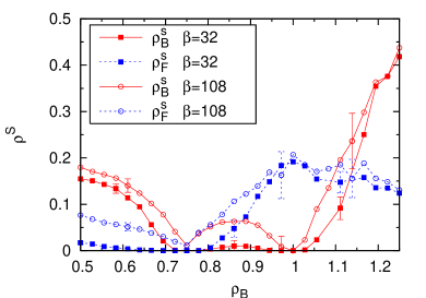
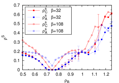
Figure 5: (Color online) “Vertical” sweep across $\rho_{B}$ at $\rho_{F}=1/4$, $U_{BB}=10$ and $U_{BF}=16$. Top panel: The boson superfluid density changes much less as $\beta$ is increased from $\beta=32$ to $\beta=108$ in the superfluid phase I at $\rho_{B}<3/4$ and $\rho_{B}>1$ than for phase III $3/4<\rho_{B}<1$. This is a hallmark of the “relay” superfluid discussed in the text. Bottom panel: The correlated winding decreases to zero at $\rho_{B}=3/4$ while the anti-correlated winding remains finite. As $\rho_{B}$ is increased beyond $3/4$ the correlated winding increases and overtakes the anti-correlated winding. This is another sign of the “relay” superfluid.

We now fill in the labeling of the phase diagram of Fig. 2. A gapless superfluid phase (I) with ($\rho^{\rm s}_{B}\neq 0$ and $\rho^{\rm s}_{F}\neq 0$) exists at low filling of the lattice $\rho_{B}+\rho_{F}<1$. When the combined filling of the two species becomes commensurate, an anti-correlated (II) phase appears in which $\rho^{\rm s}_{B}\neq 0$ and $\rho^{\rm s}_{F}\neq 0$, but $\rho^{\rm s}_{B}=\rho^{\rm s}_{F}$. This phase is characterized by superflow of the two species in opposite directions and is gapped to the addition of bosons or fermions. The usual bosonic Mott insulator, phase IV, occurs at commensurate boson densities. However, it can be melted by increasing $U_{BF}$ since the jump in bosonic chemical potential (Mott gap) is reduced to $2U_{BB}-U_{BF}$. There is no jump in $\mu_{F}$. Eventually quantum fluctuations break this gap and superflow is allowed. When $U_{BF}$ exceeds $2U_{BB}$, all superflow stops and we enter the insulating region V of the phase diagram.

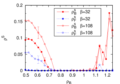
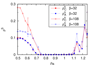
Figure 6: (Color online) “Vertical” sweep across $\rho_{B}$ at $\rho_{F}=1/4$, $U_{BB}=10$ and $U_{BF}=24$. Unlike the case for the weaker coupling $U_{BF}=16$ in Fig.  5, both superfluid densities vanish in the insulating region of the Mott lobe at commensurate total filling.

We speculate that the nature of the superfluidity in the narrow phase III, which exists between the two Mott lobes is an unusual “relay” process. It is similar to the usual superfluid which exists between Mott lobes in the single species model, in that $\rho^{\rm s}_{B}\neq 0$. However, the temperature scale at which superfluid correlations build up is dramatically reduced. This occurs because the bosons can exhibit superflow only by traveling along with a fermion partner, and being handed off from fermion to fermion in order to wind around the entire lattice. The point is that because $2U_{BB}$ exceeds $U_{BF}$ the bosons doped into the lattice above $\rho_{B}=1-\rho_{F}=3/4$ are forced to sit on a fermion. They cannot hop off, but the fermion can move since it has already paid $U_{BF}$ to share a site with a boson. Now, the fermions cannot pass each other once a fermion riding atop bosons runs into a fermion alone on a site. The fermion without a boson cannot move out of the other fermion’s way either. However, the boson sharing a site with the mobile fermion can then hop to the immobile fermion at no energy cost. Thus, the boson is passed from one fermion to the other, granting it mobility. Signatures of this phase are the lower value of the temperature at which the superfluid density builds up, that $\rho^{\rm s}_{F}>\rho^{\rm s}_{B}$, and more correlated winding than anti-correlated. However, there is nothing preventing lone fermions from acting as in the anti-correlated superfluid phase. Unfortunately this means that potential signals are masked. While we do see some of these signatures (Fig. 5) in the specified region, the numbers are not completely conclusive and will require further investigation.

VII Momentum distribution functions

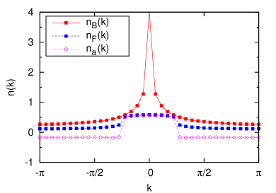
Figure 7: (Color online) I. $U_{BF}=16$, $U_{BB}=10$, $\beta=108$ and $N_{B}=20$; Momentum distributions for bosons and fermions, and Fourier transform of the anti-correlated pairing ($n_{a}(k)$) Green function. The sharp peak in bosonic momentum distribution indicates the presence of a quasi-condensate, while fermions have a plateau indicating Luttinger liquid like behavior with a clear Fermi momentum, a property that is also shared by the composite fermions described by the anti-correlated pairing.

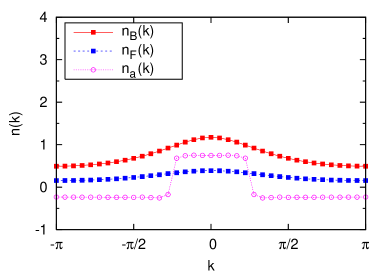
Figure 8: (Color online) II. $U_{BF}=16$, $U_{BB}=10$, $\beta=108$ and $N_{B}=27$. Bosons do not have a peak at $k=0$ and the Fermi momentum is washed out, both reflecting the onset of short range one-particle correlations. On the other hand, the plateau in the Fourier transform of the anticorrelated pairing shows that the composite fermions formed by pairing a fermion and a boson have a well defined Fermi momentum pollet06 .

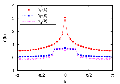
Figure 9: (Color online) III. $U_{BF}=16$, $U_{BB}=10$, $\beta=108$ and $N_{B}=32$. Qualitatively, this picture is similar to Fig. 7 - we have a peak in the bosonic momentum distribution and a plateau in the fermionic and anticorrelated pairing momentum distributions, all indicating power-law decaying correlations of their corresponding real space Green functions.

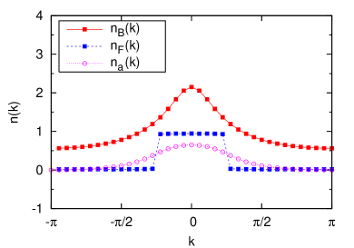
Figure 10: (Color online) IV. $U_{BF}=16$, $U_{BB}=10$, $\beta=108$ and $N_{B}=36$. There is no sharp peak in $n_{B}(k)$ and a plateau in $n_{F}(k)$ is present. This phase is a Mott Insulator for bosons and Luttinger liquid behavior for the fermions. In this case the composite fermions do not exhibit a Fermi momentum.

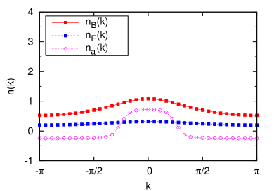
Figure 11: (Color online) V. $U_{BF}=30$, $U_{BB}=10$, $\beta=108$ and $N_{B}=27$. The momentum distribution functions in this case exhibit the behavior expected from an insulator, i.e., no sharp peak in $n_{B}(k)$, no plateau in $n_{F}(k)$, and no Fermi edge in $n_{a}(k)$.

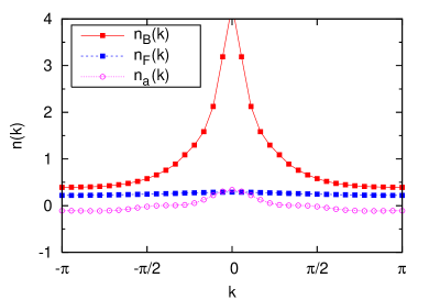
Figure 12: (Color online) VI. $U_{BF}=28$, $U_{BB}=10$, $\beta=108$ and $N_{B}=36$. Phase separation. The boson momentum distribution function has a peak indicating that there may be a kind of superflow in their separate area. Fermions, on the other hand, behave as an isolator. The $n_{a}(k)$ curve indicates that the coupling between bosons and fermions is weak, as we would expect in phase separation.

To further explore the nature of the phases we turn to the momentum distributions for the bosons, fermions, and anti-correlated pairing - Fig. 7 - 12. Each plot is made at $\beta=108$ and correspond to the parameter choices: I. $U_{BF}=16$ and $N_{B}=20$; II. $U_{BF}=16$ and $N_{B}=27$; III. $U_{BF}=16$ and $N_{B}=32$; IV. $U_{BF}=16$ and $N_{B}=36$; V. $U_{BF}=30$ and $N_{B}=27$; VI. $U_{BF}=28$ and $N_{B}=36$. In the superfluid phase (I.), there is a peak in the boson distribution and a plateau in the fermion distribution, implying quasi-condensation in the bosonic sector and Luttinger liquid-like behavior in the fermionic one. In the anti-correlated phase (II.) there is neither of the former behaviors, but the Fourier transform of the anti-correlated pairing Green function has a clear Fermi momentum showing Luttinger-like physics of the composite fermions (formed by pairing a fermions and a boson) pollet06 ; foot . The “relay” superfluid phase (III.) displays momentum distributions that are similar to the ones of superfluid phase (I). Next, in the Mott insulator / Luttinger liquid phase (IV.) one can see a clear Fermi momentum in the bare fermion $n_{F}(k)$ and a very smooth behavior of $n_{B}(k)$ and $n_{a}(k)$, which show that their real space Green function counterparts are decaying exponentially. In the insulating phase (V.) all the correlations decay exponentially and their corresponding momentum distribution functions are smooth functions of $k$. In the case of phase separation (VI.) the bosonic momentum distribution is similar to the superfluid, while fermionic distribution is insulating.

VIII Connection to previous theoretical work

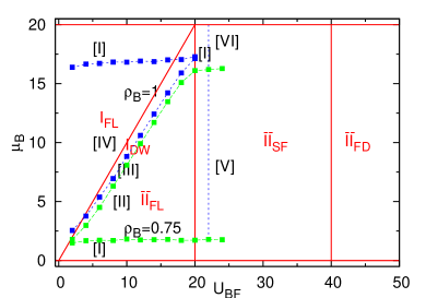
Figure 13: (Color online) A comparison of our phase diagram (Fig. 2) with the strong coupling boundaries. Symbols and dashed lines are the results of the present QMC work, while the solid lines are for $t_{B}=t_{F}=0$. Unsubscripted Roman symbols denote our phases while subscripted Roman symbols are the labeling of Lewenstein et al. lewenstein04 .

As reviewed in the introduction, there is an extensive theoretical literature on Bose-Fermi mixtures. We now make more detailed contact with previous work, first by comparing our results to the strong coupling phase diagram of Lewenstein et al. (LSBF) lewenstein04 . Fig. 13 combines our results and those of LSBF. Besides the quantitative agreement, we note the following correspondences: LSBF’s region $0\leq\bar{\mu}\leq 1$ is analogous to our $0\leq\mu\leq 20$, and $0\leq\alpha\leq 1$ to our $0\leq U_{BF}\leq 20$. Furthermore, our phase $II$ (Anti-Correlated phase) corresponds to LSBF’s phase $\bar{II}_{FL}$ (Fermi liquid of composite fermions formed by one bare fermion and bosonic hole); our phase $IV$ (Mott insulator / Luttinger liquid) to LSBF’s phase ${I}_{FL}$ (Fermi liquid); and finally our phase $III$ (Anti-Correlated phase / Relay superfluid) to LSBF’s phase ${I}_{DW}$ (Density wave phase). These three phases have similar qualities and occur approximately at the same locations at our and LSBF’s phase diagrams.

Both calculations suggest the existence of composite particles. Our phase $V$ (Insulator) corresponds to LSBF’s phase $\bar{II}_{FD}$, a region of fermionic domains of composite fermions formed by one bare fermion and bosonic hole. There is one case when the phases do not seem to correspond well, namely LSBF’s phase $\bar{II}_{SF}$ which is a superfluid of composite fermions formed by one bare fermion and bosonic hole. Our results (Fig. 3) instead suggest that in this region of $U_{BF}>2U_{BB}$, the superfluid densities vanish, or are very small.

IX Experimental issues

Albus et al. albus03 have given the correspondence between Hubbard model parameters $U_{BB},U_{BF},t_{B},t_{F}$ and experimentally controlled parameters. $U_{BB}$ and $U_{BF}$ are determined by the optical lattice depth, laser wavelength, and harmonic oscillator lengths, as well as by the scattering lengths $a_{BB}$ and $a_{BF}$ which can be tuned by traversing a Feshbach resonance. Similarly, the hoppings $t_{B}$ and $t_{F}$ follow from the lattice depth and atomic masses. It is possible to choose experimentally reasonable values of these parameters to correspond to the energy scales chosen in our paper. For example, following Albus et al, for a ${}^{87}Rb,^{40}K$ mixture and laser wavelength $600nm$, $a_{BB}=100a_{0}$, $a_{BF}=123.74a_{0}$, and $V_{0}=0.7614$ in units of boson recoil energy, with $l_{B}^{\perp}=17.04nm$, we get in units of $t_{B}$: $t_{B}=1$, $t_{F}=2$, and $U_{BB}=U_{BF}=10$. In this paper we have used $t_{B}=t_{F}=1$, which would be accessible in mixtures with $m_{F}\approx m_{B}$ such as ${}^{40}K,^{41}K$.

X Conclusions

In conclusion, we have mapped out the boson density - interaction strength phase diagram of Bose-Fermi mixtures. The Mott lobe at commensurate total density has nontrivial superfluid properties, where the two components of superflow can be nonzero and anti-correlated, or both vanish. Likewise the Mott lobe at commensurate bosonic density has vanishing boson superflow and nonzero fermion stiffness. $\rho^{\rm s}_{B}$ is nonzero upon emerging from this lobe where the balance between boson-boson and boson-fermion repulsions opens a superfluid window, with anti-correlated superflow. The superfluidity between the two Mott regions may be of a novel type where the bosons travel along with the fermions (chosen to have relatively low density in this work). As a consequence, the superfluid onset temperature is significantly reduced. Finally, we have discussed the signatures of the above phases in the momentum distribution function of fermions and bosons, which can be measured in time of flight experiments.

We acknowledge support from the National Science Foundation Grant No. ITR-0313390, Department of Energy Grant No. DOE-BES DE-FG02-06ER46319, and useful conversations with G. G. Batrouni and T. Byrds. This work is part of the research program of the Stichting voor Fundamenteel Onderzoek der materie (FOM), which is financially supported by the Nederlandse Organisatie voor Wetenschappelijk Onderzoek (NWO).

References

- (1) M. Greiner, O. Mandel, T. Esslinger, T. W. Hänsch, and I. Bloch, Nature (London) 415, 39 (2002).
- (2) D. Jaksch, C. Bruder, J. I. Cirac, C. W. Gardiner, and P. Zoller, Phys. Rev. Lett. 81, 3108 (1998).
- (3) H. Ott, E. de Mirandes, F. Ferlaino, G. Roati, G. Modugno, and M. Inguscio, Phys. Rev. Lett. 92, 160601 (2004).
- (4) K. Günter, T. Stöferle, H. Moritz, M. Köhl, and T. Esslinger, Phys. Rev. Lett. 96, 180402 (2006).
- (5) S. Ospelkaus, C. Ospelkaus, L. Humbert, K. Sengstock, and K. Bongs, Phys. Rev. Lett. 97, 120403 (2006).
- (6) M. Zaccanti, C. D’Errico, F. Ferlaino, G. Roati, M. Inguscio, and G. Modugno, Phys. Rev. A 74, 041605(R) (2006).
- (7) M. A. Cazalilla and A. F. Ho, Phys. Rev. Lett. 91, 150403 (2003).
- (8) M. Lewenstein, L. Santos, M. A. Baranov, and H. Fehrmann, Phys. Rev. Lett. 92, 050401 (2004).
- (9) L. Mathey, D.-W. Wang, W. Hofstetter, M. D. Lukin, and E. Demler, Phys. Rev. Lett. 93, 120404 (2004); L. Mathey and D.-W. Wang, Phys. Rev. A 75, 013612 (2007).
- (10) A. Imambekov and E. Demler, Phys. Rev. A 73, 021602(R) (2006).
- (11) L. Pollet, M. Troyer, K. Van Houcke, and S. M. A. Rombouts, Phys. Rev. Lett. 96, 190402 (2006).
- (12) P. Sengupta and L. P. Pryadko, Phys. Rev. B 75, 132507 (2007).
- (13) F. Hébert, F. Haudin, L. Pollet, and G. G. Batrouni, Phys. Rev. A 76, 043619 (2007).
- (14) A. Albus, F. Illuminati, and J. Eisert, Phys. Rev. A 68, 023606 (2003).
- (15) M. Cramer, J. Eisert, and F. Illuminati, Phys. Rev. Lett. 93, 190405 (2004).
- (16) L. Pollet, C. Kollath, U. Schollwöck, and M. Troyer, Phys. Rev. A 77, 023608 (2008).
- (17) A. Mering and M. Fleischhauer, Phys. Rev. A 77, 023601 (2008).
- (18) V. G. Rousseau and P. J. H. Denteneer, Phys. Rev. A 77, 013609 (2008).
- (19) M. P. A. Fisher, P. B. Weichman, G. Grinstein, and D. S. Fisher, Phys. Rev. B 40, 546 (1989).
- (20) K. Van Houcke, S. M. A. Rombouts, and L. Pollet, Phys. Rev. E 73, 056703 (2006).
- (21) S. M. A. Rombouts, K. Van Houcke, and L. Pollet, Phys. Rev. Lett. 96, 180603 (2006).
- (22) G. G. Batrouni, R. T. Scalettar, and G. T. Zimanyi, Phys. Rev. Lett. 65, 1765 (1990).
- (23) N. V. Prokof’ev, B. V. Svistunov, and I. S. Tupitsyn, JETP 87, 310 (1998).
- (24) Unlike , which is the length of a vector and hence must be positive, there is no such constraint on , which is the Fourier transform of . We have verified that the same small negative values of in the figures are also obtained in exact diagonalization on small clusters.