Fractal Threshold Behavior in Vacuum Gravitational Collapse

Abstract

We present the numerical evidence for fractal threshold behavior in the five dimensional vacuum Einstein equations satisfying the cohomogeneity-two triaxial Bianchi type-IX ansatz. In other words, we show that a flip of the wings of a butterfly may influence the process of the black hole formation.

Introduction.—Critical phenomena in gravitational collapse are an interdisciplinary field that was initiated by the remarkable work of Choptuik PhysRevLett.70.9 . It concerns the study of the basin boundary between two generic states — space-times with and without black holes. This bistable behavior shares many properties with the phase transition in statistical mechanics. It is a well-known fact that, in general, basin boundaries can be either smooth or fractal, and there is no reason to believe that gravity is special in this context. However, in more than one hundred papers that were devoted to critical phenomena in gravitational collapse so far Gundlach:2002sx ; LR2007 , the basin boundary between dispersion and collapse to a black hole is always smooth, and there is no indication of chaos footnote1 . The single counterexample Szybka:2003uz is restricted to the solution with many unstable modes and as such it does not give a chance to observe fractal threshold behavior directly in the initial value problem.

The theory of chaos in infinite dimensional systems is not fully developed yet, but this field is of great interest and growing rapidly. In this Letter we provide an example of chaos in reduced Einstein equations that constitute a system of partial differential equations. We clarify the hypothesis of Bizoń et al. Bizon:2006qi and present fractal threshold behavior that can be interpreted as a chaotic scattering in a critical surface—the surface in the phase space of initial data that separate collapse to a black hole from dispersion. This surface is smooth, but it contains three copies of the critical solution, and the basin sets of these copies have fractal boundaries. In this sense, the chaotic behavior presented here is double critical and can be directly seen in the dynamical evolution. In our Letter we estimate the fractal dimension of the basin boundaries. The fractal dimension is a diffeomorphism invariant indicator of chaos in general relativity mixmaster .

Setting.—We consider vacuum gravitational collapse in a very simple setting. Namely, in order to evade Birkhoff’s theorem and save radial symmetry, we take five dimensional vacuum Einstein equations and reduce the number of degrees of freedom by the BCS ansatz Bizon:2005cp , Bizon:2006qi

$$ds^{2} \!=\! -Ae^{-2\delta}dt^{2}+A^{-1}dr^{2}$$ (1)

$$+\frac{1}{4}r^{2}\left[e^{2B}\sigma_{1}^{2}\!+\!e^{2C}\sigma_{2}^{2}\!+\!e^{-2(B+C)}\sigma_{3}^{2}\right],$$

where $A$, $\delta$, $B$, and $C$ are functions of time $t$ and radius $r$. One-forms $\sigma_{k}$ are standard left-invariant one-forms on $SU(2)$,

$$\sigma_{1}+i\,\sigma_{2}=e^{i\psi}(\cos{\theta}\;d\phi+i\,d\theta),\quad\sigma_{3}=d\psi-\sin{\theta}\;d\phi,$$ (2)

where $0\leq\theta\leq\pi$, $0\leq\phi\leq 2\pi$, and $0\leq\psi\leq 4\pi$ are Euler angles. The angular part of the metric (1) corresponds to the spatial part of the metric in Bianchi IX cosmology. $SU(2)$ is dipheomorphic to $S^{3}$; therefore $B$ and $C$ functions can be interpreted as squashing parameters of $S^{3}$. $B=C=0$ correspond to the round $S^{3}$ and $B=C\neq 0$ to the deformed $S^{3}$ with one squashing parameter (the so-called biaxial case). In this Letter we consider the triaxial case where $B$, $C$ are independent functions—two dynamical degrees of freedom. The vacuum Einstein equations derived for the metric (1) (see Bizon:2006qi ) possess a discrete $Z_{3}$ symmetry. It corresponds to the freedom of permutations of coefficients of one-forms $\sigma_{k}$ in the angular part of the metric (1). These permutations are generated by the following transpositions:

$$T_{12}:(B,C)\rightarrow(C,B),\quad T_{23}:(B,C)\rightarrow(B,-B-C),$$

$$T_{13}:(B,C)\rightarrow(-B-C,C)\,,$$ (3)

where the transposition $T_{ij}$ swaps the coefficients of $\sigma_{i}^{2}$ and $\sigma_{j}^{2}$ in (1). Biaxial configurations correspond to the fixed points of these transpositions: $(B,B)$, $(B,-B/2)$, and $(B,-2B)$. All biaxial solutions exist in three geometrically equivalent copies.

Critical phenomena.—The study Bizon:2005cp of the critical phenomena in the model restricted to biaxial symmetry revealed type-II gravitational collapse with the critical solution being discretely self-similar ($DSS$). It was also shown Bizon:2006qi that in triaxial symmetry the phenomenology of critical behavior remains the same. The $Z_{3}$ symmetry implies that in the triaxial case the critical solution (hereafter denoted as $DSS_{1}$—because it is discretely self-similar and has one unstable mode) takes one of three equivalent forms. Let us denote them as $X_{1}^{(1)}$, $X_{2}^{(1)}$ and $X_{3}^{(1)}$. Each of these copies acts as a codimension-one attractor in the phase space of solutions. Hence, the codimension-one critical surface $\mathcal{M}_{crit}$ contains three basin sets $\mathcal{M}_{i}$ ($i=1,2,3$). It was shown by Bizoń et al.  Bizon:2006qi that the basin boundaries of these sets are given by the stable manifolds of the discretely self-similar codimension-two attractor $DSS_{2}$. Moreover, the authors suggested that the basin boundaries could be fractal.

In this Letter we continue the work that was initiated in Bizon:2006qi and investigate the structure of the basin boundaries of codimension-one attractors $X_{i}^{(1)}$. In other words, we study numerically the Cauchy problem for two-parameter families of initial data. We fine-tune one of the parameters to the critical surface $\mathcal{M}_{crit}$ and the remaining parameter to the basin boundary (this means fine-tuning to the codimension-two attractor $DSS_{2}$).

One of the problems in carrying on such studies numerically comes from the fact that in order to cancel two growing modes of $DSS_{2}$ in general two-parameter initial data, one is forced to use very high numerical precision. It leads, on the software level, to the necessity of multiprecision packages. These packages slow down the numerical evolution, and the calculations become computationally infeasible. The possible solution is to find special two-parameter initial data that are convenient in the study of the basin boundaries in $\mathcal{M}_{crit}$. We propose the following procedure for finding such initial data.

Let us consider general initial data that are fine-tuned to $DSS_{2}$. The solution generated by such initial data approach $DSS_{2}$ and, since it is always fine-tuned with a finite precision, repels from $DSS_{2}$. However, one can freeze the evolution at the moment the solution is “nearly” $DSS_{2}$. Using this snapshot one can generate another two-parameter family of initial data.

In particular, we consider time-symmetric initial data that were studied in Bizon:2006qi :

$$B(0,r)=p\,f(r),\quad C(0,r)=a\,B(0,r),$$ (4)

where $f(r)=100\,r^{2}\exp[-20(r-0.1)^{2}]$ is the generalized Gaussian (for details, see Bizon:2006qi ). In order to fine-tune to $DSS_{2}$ we set parameters

$$\begin{array}[]{ll}a=0.1411036683285,\\ p=0.09524484187150217214296769,\end{array}$$ (5)

and evolve the solution up to $\tilde{t}=1.038$. Next, we introduce two new parameters $\kappa$, $\iota$ and rescale $\hat{C}(\tilde{t},r)=\kappa C(\tilde{t},r)$, $\hat{B}(\tilde{t},r)=\iota B(\tilde{t},r)$. In this way we create a new, two-parameter ($\kappa$, $\iota$) family of initial data.

Figure 1: The critical surface $\mathcal{M}_{crit}$ presented in the phase space of parameters $\kappa$ and $\iota$. All initial conditions defined by $\iota^{*}(\kappa)$ lead to the solutions that approach the critical solution $DSS_{1}$ or attractors of higher codimension ($DSS_{2}$ or possibly others). $\iota\gtrapprox\iota^{*}$ leads to supercritical solutions (with a black hole) and $\iota\lessapprox\iota^{*}$ gives subcritical solutions (dispersion). The error bars are lower than $10^{-5}$.

Hereafter we restrict our analysis only to this particular family. The critical surface $\mathcal{M}_{crit}$ corresponds to a curve $\iota^{*}(\kappa)$ in the parameter space. We present this curve in Fig. 1.

In order to characterize evolution of initial data given by $\iota^{*}(\kappa)$ we define below a map $h:\kappa\in\mathbb{R}\rightarrow a\in\{1,-\frac{1}{2},-2,0\}$. Generic solutions starting from $\iota^{*}(\kappa)$ approach one of the codimension-one attractors $X_{1}^{(1)}$, $X_{2}^{(1)}$, $X_{3}^{(1)}$ and recover biaxial symmetry $C=aB$ in one of three equivalent forms: $a=1$, $a=-\frac{1}{2}$, $a=-2$, respectively. Moreover, there are points that separate basins of attraction $\mathcal{M}_{i}$. For a practical convenience we denote them as $a=0$, but we stress that this is not related to the scaling $C=aB$. The set of all such points forms the basin boundary $Q$. It was shown in Bizon:2006qi that solutions defined by $Q$ approach the $DSS_{2}$ solution or possibly higher codimension attractors. The map $h:\kappa\rightarrow a$ describes asymptotic behavior of solutions, but in finite precision numerical calculations it describes intermediate dynamics. Such calculations show that if $\kappa_{A}<\kappa_{B}$ and $h(\kappa_{A})\neq h(\kappa_{B})$, and $h(\kappa_{A})h(\kappa_{B})\neq 0$, then there exists $\kappa_{Q}$ such that $\kappa_{A}<\kappa_{Q}<\kappa_{B}$ and $h(\kappa_{Q})=0$. Again, in practical calculations we mark by $h(\kappa)=0$ all points with an undetermined basin set. For these points the double precision of the parameter $\iota^{*}$ is not sufficient to cancel by a bisection the $\mathcal{M}_{crit}$-transversal growing mode of $DSS_{2}$. This mode dominates over the $\mathcal{M}_{crit}$-tangential growing mode of $DSS_{2}$ and the $DSS_{1}$ behavior is not observed. In contrast to this, for $h(\kappa)\neq 0$ the $\mathcal{M}_{crit}$-tangential growing mode of $DSS_{2}$ takes over and “pushes” solutions along $\mathcal{M}_{crit}$. Such solutions approach one of the copies of $DSS_{1}$. Finally, since the bisection has a finite precision, they are also repelled from $\mathcal{M}_{crit}$ along the unstable mode of $DSS_{1}$. This behavior was described in detail in Bizon:2006qi .

To study the geometry of $\mathcal{M}_{crit}$, especially the geometry of basin sets $\mathcal{M}_{i}$, we determined the map $h$ in the numerical experiment. We have collected two samples corresponding to two scales in the basin boundary. Sample $1$ contains $15001$ points and corresponds to $\kappa\in S_{1}=[-0.5,1]$. Sample $2$ contains $3201$ points and corresponds to $\kappa\in S_{2}=[0.07,0.078]$. All test points were uniformly distributed in respective intervals.

It is clearly seen in Fig. 2 that the basin boundaries have a complex structure footnote2 . Magnifying a part of the boundary reveals a new structure presented in Fig. 3. Therefore, one should expect that an intersection of the basin boundary $Q$ with tested sets $S_{1}$, $S_{2}$ has nontrivial fractal dimension $0<dim(S_{i}\cap Q)<1$, where $i=1,2$. In order to estimate the fractal dimension we follow 1983PhLA…99..415G ; fractalbb and calculate the uncertainty dimension footnote3 (from now on $dim$ denotes the uncertainty dimension).

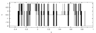
Figure 2: Sample $1$. The type of the $DSS_{1}$ solution as a function of $\kappa$ (plotted as a histogram). $h(\kappa)=1$, $h(\kappa)=-1/2$, $h(\kappa)=-2$ correspond to $X_{1}^{(1)}$, $X_{2}^{(1)}$, $X_{3}^{(1)}$, respectively, and $h(\kappa)=0$ corresponds to points with an undetermined basin.

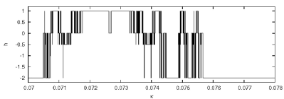
Figure 3: Sample $2$. Part of Fig. 2 magnified. The complex structure is seen at a different scale.

Let $S$ be a one-dimensional set in one-dimensional parameter phase space (we have one free parameter $\kappa$). The probability that any two random points $\kappa_{A}$, $\kappa_{B}$ separated by a distance $\epsilon$ belong to different basins $h(\kappa_{A})\neq h(\kappa_{B})$ scales as $P(\epsilon)\sim\epsilon^{1-dim(S\cap Q)}$. Testing many pairs of points for several values of $\epsilon$ one can fit $P(\epsilon)$ to the power law and estimate $dim(S\cap Q)$. The wider the range of $\epsilon$ we consider (assuming $\epsilon$ is small enough), the higher precision we obtain.

Figure 4: Sample $1$. $P$ is a probability that any two random points $\kappa_{A}$, $\kappa_{B}$ separated by a distance $\epsilon$ belong to different basins $h(\kappa_{A})\neq h(\kappa_{B})$. The uncertainty dimension was estimated to be $dim(S_{1}\cap Q)=1-w=0.722\pm 0.006$, where $w$ is a slope of the linear fit above.

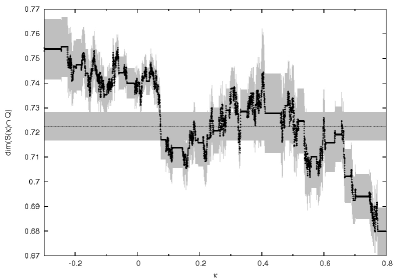
Figure 5: The uncertainty dimension $dim(S(\kappa)\cap Q)$ varies with $\kappa$. The set $S(\kappa)=[\kappa-0.2,\kappa+0.2]$ contains $4001$ points for each value of $\kappa$. The horizontal dotted line indicates averaged uncertainty dimension $dim(S_{1}\cap Q)$. The gray area represents errors.

The fit to the power law for Sample $1$ presented in Fig. 4 reveals that $dim(S_{1}\cap Q)=0.722\pm 0.006$, therefore the basin boundary is fractal. However, the quantity estimated above is an “averaged” fractal dimension. In order to see this, let us consider a set $S(\kappa)=[\kappa-0.2,\kappa+0.2]$ and $dim(S(\kappa)\cap Q)$ for $\kappa$ such that $S(\kappa)\subset S_{1}$. It follows from Fig. 5 that the uncertainty dimension $dim(S(\kappa)\cap Q)$ varies with $\kappa$, so the investigated structure seems to be a multifractal rather than a monofractal. Such hypothesis is supported by the fractal dimension of Sample $2$, namely $dim(S_{2}\cap Q)=0.680\pm 0.006$ (see the linear fit in Fig. 6). It follows from the definition of the uncertainty dimension that $S_{2}\subset S_{1}\Rightarrow dim(S_{1}\cap Q)\geq dim(S_{2}\cap Q)$. The estimated values satisfy this inequality as expected. The smaller $\epsilon$ we take, the more precise bisection we need and more quickly the numerical double precision of $\iota^{*}$ is exhausted. Therefore, Sample $2$ contains ca. $18\%$ of points with an undetermined basin in contrast to only ca. $7\%$ in case of Sample $1$. Clearly, the finite precision of the bisection makes the number of points with an undetermined basin scale dependent and may have a greater effect on the fractal dimension of Sample $2$. The error bars shown in Figs. 4 and 6 indicate statistical errors 1983PhLA…99..415G .

The multifractal objects can be more completely characterized by the singularity spectrum, but such analysis of our system would involve more precise data and an enormous computational power. Let us mention that the computer resources needed to collect Sample $1$ and Sample $2$ involved over six dozens of processors with the integration time measured in weeks.

The direct analogy to finite dimensional dynamical systems suggests that the $DSS_{2}$ solution plays a role of a strange repeller bgo , but we do not have sufficient dynamical evidence to support such claim. To the best of our knowledge, the nature of solutions that drive the dynamics in a fractal basin boundary remains unknown in the context of partial differential equations tc . A construction of the $DSS_{2}$ solution in Bizon:2006qi is a first example that may give some insight into this problem.

Conclusions.—In summary, we have presented the numerical results that indicate the presence of fractal basin boundaries in the critical surface in five dimensional vacuum gravitational collapse. Moreover, the data support the hypothesis that basin boundaries are multifractals. We note that all three copies of the critical solution ($X_{1}^{(1)}$, $X_{2}^{(1)}$ and $X_{3}^{(1)}$) are geometrically equivalent. Therefore, one should not expect to see chaos in the black hole mass scaling of supercritical solutions. The solutions behave chaotically in the nearly double-critical regime, and then settle down to the Minkowski space-time or the black hole. This final state is not sensitive to initial conditions, but the way in which it is approached is, indeed, chaotic.

Figure 6: Sample $2$. The uncertainty dimension was estimated to be $dim(S_{2}\cap Q)=1-w=0.680\pm 0.006$, where $w$ is a slope of the linear fit above.

Acknowledgments.—We thank Piotr Bizoń for a helpful discussion and Zbisław Tabor for letting us adapt his code. The numerical experiments presented here were performed on machines of Interdisciplinary Centre for Mathematical and Computational Modelling at Warsaw University (ICM, Grant No. G32-6), Academic Computer Centre Cyfronet AGH (Grant No. MNiSW/IBM_BC_HS21/UJ/104/2007), Astronomical Observatory UJ, Institute of Physics UJ and Henryk Niewodniczański Institute of Nuclear Physics PAN. This research was also supported by MNiSW Grant No. 1 P03B 012 29.

References

- (1) M. W. Choptuik, Phys. Rev. Lett. 70, 9 (1993).
- (2) C. Gundlach, Phys. Rep. 376, 339 (2003), gr-qc/0210101.
- (3) C. Gundlach and J. M. Martín-García, Living Rev. Relativity 10, 5 (2007), www.livingreviews.org/lrr-2007-5.
- (4) For the possibility of chaos in critical phenomena in black holes collisions see Levin ; LR2007 .
- (5) J. Levin, Phys. Rev. Lett. 84, 3515 (2000), gr-qc/9910040.
- (6) S. J. Szybka, Phys. Rev. D 69, 084014 (2004), gr-qc/0310050.
- (7) P. Bizoń, T. Chmaj, and B. G. Schmidt, Phys. Rev. Lett. 97, 131101 (2006), gr-qc/0608102.
- (8) N. J. Cornish, J. J. Levin, Phys. Rev. Lett. 78, 998 (1997), gr-qc/9605029.
- (9) P. Bizoń, T. Chmaj, and B. G. Schmidt, Phys. Rev. Lett. 95, 71102 (2005), gr-qc/0506074.
- (10) All three possible types of behavior are present in the neighborhood of the boundary. It would be interesting to verify if the basin boundary has the so-called Wada property—any point which is on the boundary of one basin set is also simultaneously on the boundary of all other basin sets.
- (11) C. Grebogi, S. W. McDonald, E. Ott, and J. A. Yorke, Phys. Lett. A 99, 415 (1983).
- (12) S. W. McDonald, C. Grebogi, E. Ott, and J. A. Yorke, Physica (Amsterdam) 17D, 125 (1985).
- (13) The uncertainty dimension, the box-counting dimension, and Hausdorff dimension are equal for one and two dimensional systems that are uniformly hyperbolic on their basin boundary 1992CMaPh.150….1N .
- (14) H. E. Nusse and J. A. Yorke, Commun. Math. Phys. 150, 1 (1992).
- (15) S. Bleher, C. Grebogi, and E. Ott, Physica (Amsterdam) 46D, 87 (1990).
- (16) S. R. Taylor and S. A. Campbell, Phys. Rev. E 75, 046215 (2007).