Spin Transfer Torques

Abstract

This tutorial article introduces the physics of spin transfer torques in magnetic devices. We provide an elementary discussion of the mechanism of spin transfer torque, and review the theoretical and experimental progress in this field. Our intention is to be accessible to beginning graduate students. This is the introductory paper for a cluster of “Current Perspectives” articles on spin transfer torques published in volume 320 of the Journal of Magnetism and Magnetic Materials. This article is meant to set the stage for the others which follow it in this cluster; they focus in more depth on particularly interesting aspects of spin-torque physics and highlight unanswered questions that might be productive topics for future research.

url]http://people.ccmr.cornell.edu/$\sim$ralph/ url]http://cnst.nist.gov/epg/epg_home.html

1 Introduction

The electrons that carry charge current in electronic circuits also have spins. In non-ferromagnetic samples, the spins are usually randomly oriented and do not play a role in the behavior of the device. However, when ferromagnetic components are incorporated into a device, the flowing electrons can become partially spin polarized and these spins can play an important role in device function. Due to spin-based interactions between the ferromagnets and electrons, the orientations of the magnetization for ferromagnetic elements can determine the amount of current flow. By means of these same interactions, the electron spins can also influence the orientations of the magnetizations. This last effect, the so-called spin transfer torque, is the topic of the following series of articles. The goal of these articles is to provide an introduction to the topical scientific issues concerning the theories, experiments, and commercial applications related to spin transfer torques. These articles are written by some of the leaders in the study of spin transfer torques and we hope that they will be useful to beginning students starting their study as well as of interest to experts in the field.

The authors of the succeeding articles were asked to consider the field from their particular point of view, and to provide a “preview” – including discussion of interesting unsolved problems – rather than merely a review of completed work. Hopefully, when taken together these articles provide a broad and representative view of where the field is and where it may be going.

The goal of the present article is to provide basic background and context for the succeeding articles. We start with a very brief history of the field and provide references to background material. Then, in Section 2, we introduce aspects of ferromagnetism that are important to the discussion, particularly for transition-metal ferromagnets, and discuss how spin polarized currents arise. Section 3 describes how spin transfer torques can be understood as resulting from changes in spin currents. Section 4 explains some of the issues associated with how spin transfer torques affect magnetic-multilayer devices and tunnel junctions. Section 5 describes how they affect domain walls in magnetic nanowires. Finally, Section 6 introduces the succeeding articles in the context provided by the rest of this article.

The first work to consider the existence of spin transfer torques occurred in the late 1970’s and 1980’s, with Berger’s prediction that spin transfer torques should be able to move magnetic domain walls [1], followed by his group’s experimental observations of domain-wall motion in thin ferromagnetic films under the influence of large current pulses [2, 3]. The phenomenon did not attract a great deal of attention at the time, largely because very large currents (up to 45 A!) were required, given that the samples were quite wide – on the scale of mm. However, with advances in nanofabrication techniques, magnetic wires with 100 nm widths can now be made readily, and these exhibit domain wall motion at currents of a few mA and below. Research on spin-transfer-induced domain wall motion has been pursued vigorously by many groups since the early days of the 21st century [4, 5, 6, 7, 8]. The present state of studies of spin-torque-driven domain wall motion is described in the articles by Beach, Tsoi, and Erskine, by Tserkovnyak, Brataas, and Bauer, and by Ohno and Dietl.

Widespread interest in magnetic nanostructures began in 1986 with the discovery of interlayer exchange coupling [9, 10, 11]. Interlayer exchange coupling [12] is the interaction between the magnetizations of two ferromagnetic layer separated by an ultrathin, non-ferromagnetic spacer layer. Of particular interest was the discovery of antiferromagnetic coupling in the Fe/Cr/Fe system by Grünberg et al. because it led shortly thereafter to the discovery of the Giant Magnetoresistance (GMR) effect by Grünberg’s group and Fert’s group [13, 14]. Grünberg and Fert shared the 2007 Nobel Prize in Physics for this discovery. GMR is the change in resistance that occurs when the relative orientation of the magnetizations in two ferromagnetic layers changes. For example, when the magnetizations of two Fe layers separated by Cr are antiparallel to each other as they are when antiferromagnetically coupled, the sample has a relatively large resistance. The magnetizations of the Fe layers can be brought into parallel alignment by an external magnetic field, and this decreases the resistance. At intermediate angles, the resistance is also intermediate between these maximum and minimum values. See Fig. 1. The overall size of the change in resistance is typically up to a few 10’s of percent, which is “giant” compared to the $\approx$ 1 % magnetoresistance changes of pure magnetic metals by themselves (due to anisotropic magnetoresistance [15]). Most of the early work on GMR focused on the sample geometry in which the current flows in the plane (CIP) of the multilayer sample. Another geometry, first explored in 1991 [16] has the current flow perpendicular to the planes (CPP) of the multilayer and gives larger fractional resistance changes [17]. The CPP geometry is of particular interest in the present context because spin transfer effects are more important than they are in the CIP geometry.

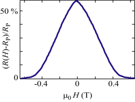
Figure 1: Giant Magnetoresistance (GMR) of a multilayer film with the structure (1.2 nm Co / 0.96 nm Cu)₁₀. The measurement is done with the current flowing in the sample plane at a temperature of 4.2 K. The resistance is large near zero magnetic field where the interlayer exchange coupling between adjacent Co layers aligns their magnetizations antiparallel. The resistance decreases as an applied magnetic field rotates the magnetizations to become parallel to each other. $R_{\rm P}$ is the resistance when the two magnetizations are parallel. Data are courtesy of Jordan Katine.

In studying the GMR effect, Parkin et al. discovered in 1990 that the interlayer exchange coupling oscillates as a function of the thickness of the spacer layer [18]. The oscillations could be quite dramatic; up to sixty changes in sign of the coupling were seen in single wedge-shaped samples allowing the simultaneous study of a range of thicknesses [19]. Comparison of the oscillations with calculations [20] confirmed that this coupling was an exchange interaction mediated by the electrons in the spacer layer and that the oscillation periods were determined by the geometry of the spacer layer’s Fermi surface.

In 1989, Slonczewski [21] calculated the interlayer exchange coupling for the case in which the spacer layer is an insulating tunnel barrier. While there were no measurements of exchange coupling across insulators at the time, his article has two features of particular interest in regard to spin-torque physics. First, Slonczewski calculated the exchange coupling by determining the spin current flowing through the tunnel barrier. A spin current flows even with zero applied bias across the tunnel junction whenever the magnetizations of the two electrodes are non-collinear, and the source of the exchange coupling can be understood to be the transfer of angular momentum from this spin current to each magnet. The second feature of interest is that he considered the additional coupling that results when a voltage is applied across the junction. This was the first calculation of a spin transfer torque in a multilayer geometry with current flowing perpendicular to the plane. However, there was little immediate experimental follow-up, because the technology for making magnetic tunnel junctions at that time was still rather primitive, and provided only tunnel barriers that were too thick to permit the large current densities needed to excite spin-torque-driven magnetic dynamics.

The papers most influential in launching the study of spin transfer torques came in 1996, when Slonczewski [22] and Berger [23] independently predicted that current flowing perpendicular to the plane in a metallic multilayer can generate a spin transfer torque strong enough to reorient the magnetization in one of the layers. Since the metallic magnetic multilayers used for GMR studies have low resistances (compared to tunnel barriers), they could easily sustain the current densities required for spin transfer torques to be important. Slonczewski predicted that the spin transfer torque from a direct current could excite two qualitatively different types of magnetic behaviors depending on the device design and the magnitude of an applied magnetic field: either simple switching from one static magnetic orientation to another or a dynamical state in which the magnetization undergoes steady-state precession. His subsequent 1997 patent [24] was remarkably far-seeing, providing detailed predictions for many of the applications that are currently being pursued.

Measurements of current-induced resistance changes in magnetic multilayer devices were first identified with spin-torque-driven excitations in 1998 by Tsoi et al., for devices consisting of a mechanical point contact to a metallic multilayer [25], and in 1999 by Sun in manganite devices [26]. Observation of magnetization reversal caused by spin torques in lithographically defined samples occurred shortly thereafter [27, 28]. Fig. 2 shows comparisons between spin-torque-driven magnetic switching and magnetic-field driven switching for a metallic multilayer and a magnetic tunnel junction. Phase-locking between spin-torque-driven magnetic precession and an alternating magnetic field was detected in 2000 [29] and direct measurements of steady-state high-frequency magnetic precession caused by spin torque from a direct current were made beginning in 2003 [30, 31, 32]. Figure 3 shows an example of voltage oscillations due to spin-torque-driven magnetic precession. The article by Berkov and Miltat describes some of these results and shows to what extent it is currently possible to make a detailed comparison between theory and experiment. The article by Silva and Rippard discusses some of the open questions pertaining to spin-torque-driven precession in the point-contact sample geometry.

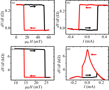
Figure 2: Comparison of magnetic switching at room temperature as driven by applied magnetic fields and by spin transfer torques. (a) Switching for an all-metal nanopillar sample consisting of the layers 20 nm Ni₈₁Fe₁₉ / 12 nm Cu / 4.5 nm Ni₈₁Fe₁₉, as the magnetization of the thinner (free) magnetic layer is aligned parallel and antiparallel to the thicker magnetic layer by an applied magnetic field. (b) Spin-torque-driven switching by an applied current in the same device, with a constant magnetic field applied to give zero total field acting on the free layer. (c) Switching for a magnetic tunnel junction nanopillar sample consisting of the layers 15 nm PtMn / 2.5 nm Co₇₀Fe₃₀ / 0.85 nm Ru / 3 nm Co₆₀Fe₂₀B₂₀ / 1.25 nm MgO / 2.5 nm Co₆₀Fe₂₀B₂₀, as the 2.5-nm Co₆₀Fe₂₀B₂₀ free layer is reversed by an applied magnetic field. (d) Spin-torque-driven switching by an applied current in the same tunnel junction, with a constant magnetic field applied to give zero total field acting on the free layer. Data for (a) and (b) are from [146], and data for (c) and (d) are courtesy of Jonathan Sun.

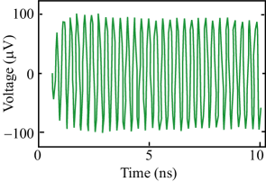
Figure 3: Voltage oscillations produced by steady-state precession of the magnetic free layer in a nanopillar sample, in response to the spin transfer torque from a 8.4 mA current step. The sample had the layer structure 8 nm Ir₂₀Mn₈₀ / 4 nm Ni₈₀Fe₂₀ / 8 nm Cu / 4 nm Ni₈₀Fe₂₀, with the direction of the exchange bias from the Ir₂₀Mn₈₀ layer oriented 45^∘ from the easy axis of the upper Ni₈₀Fe₂₀ free layer. The measurement was made at a temperature of 40 K using a sampling oscilloscope [32].

At the same time that interest was beginning to grow regarding spin transfer torques in metallic multilayers, so was the interest in magnetic tunnel junctions, starting with the observation in 1995 of substantial tunnel magnetoresistance (TMR, the difference in resistance between parallel and antiparallel orientation for the electrode magnetizations of a magnetic tunnel junction) at room temperature [33, 34]. Most of the early studies used aluminum oxide as a tunnel barrier. Since aluminum oxide barriers are heavily disordered it is difficult to study them theoretically. In 2001, Butler et al. and Mathon and Umerski calculated the tunneling properties of the Fe/MgO/Fe system [35, 36], which can be lattice-matched and potentially well-ordered. They found that the symmetry of the system and the relevant electronic states lead to the possibility of an extremely large TMR. In 2004, values of TMR greater than those observed for aluminum oxide barriers were published [37, 38] and the values of TMR demonstrated experimentally have continued to increase rapidly until this day.

Techniques have now been developed to make both aluminum oxide and MgO tunnel barriers sufficiently thin to support the current densities needed to produce magnetic switching with spin transfer torques [39, 40, 41]. Work is underway to investigate spin-torque-driven precession in tunnel barriers, as well. One reason for the interest in spin-torque effects in tunnel junctions is that tunnel junctions are better-suited than metallic magnetic multilayers for many types of applications. Tunnel junctions have higher resistances that can often be better impedance-matched to silicon-based electronics, and TMR values can now be made larger than the GMR values in metallic devices. The science and technology of spin transfer torques in tunnel junctions are discussed in the articles by Katine and Fullerton and by Sun and Ralph.

The possibility of commercial application has been a strong driving force in this field from the beginning. Grünberg [42] filed a German patent for applications of GMR in 1988 even before the effect was published in the scientific literature, and the phrase “giant magnetoresistance” now appears in over 1500 US patents. Devices based on the GMR and TMR effects have already found very widespread application as the magnetic-field sensors in the read heads of magnetic hard disk drives, and a non-volatile random access memory based on magnetic tunnel junctions has recently been introduced. Slonczewski’s 1997 patent [24] for devices based on spin transfer torques has been referenced by 64 subsequent patents. Applications of spin transfer torques are envisioned using both types of magnetic dynamics that spin torques can excite. Magnetic switching driven by the spin transfer effect can be much more efficient than switching driven by current-induced magnetic fields (the mechanism used in the existing magnetic random access memory). This may enable the production of magnetic memory devices with much lower switching currents and hence greater energy efficiency and also greater device density than field-switched devices. The steady-state magnetic precession mode that can be excited by spin transfer is under investigation for a number of high-frequency applications, for example nanometer-scale frequency-tunable microwave sources, detectors, mixers, and phase shifters. One potential area of use is for short-range chip-to-chip or even within-chip communications. Spin-torque-driven domain wall motion is also under investigation for memory applications. Parkin has proposed a “Racetrack Memory” [43] which envisions storing bits of information using many domains arranged sequentially in a magnetic nanowire and retrieving the information by using spin transfer torques to move the domains through a read-out sensor. The article by Katine and Fullerton discusses in detail the opportunities and challenges for potential applications.

There are several books that can provide more background information for this set of articles on spin transfer torques. One resource is the four volume series Ultrathin Magnetic Structures edited by Heinrich and Bland [44]. These volumes contain articles on almost all aspects of magnetic thin films and devices made out of them. Another useful book, written at a more pedagogical level, is Nanomagnetism: Ultrathin Films, Multilayers and Nanostructures, edited by Mills and Bland [45]. The three volume series Spin Dynamics in Confined Magnetic Structures edited by Hillebrands, Ounadjela, and Thiaville covers dynamical aspects of magnetic nanostructures [46]. The five volume set, Handbook of Magnetism and Advanced Magnetic Materials, edited by Kronmüller and Parkin, covers the entire field of magnetism including the topics of interest here [47]. Concepts in Spin Electronics, edited by Maekawa, provides another recent overview [48]. Finally, The Journal of Magnetism and Magnetic Materials published a collection of review articles including several on topics related to magnetic multilayers in Volume 200 [49]. Specific chapters in these books and other review articles on spin transfer torques will be mentioned throughout this article.

2 The Basics of Ferromagnetism

The Origin of Ferromagnetism. Ferromagnetism occurs when an electron system becomes spontaneously spin polarized. In transition metals, ferromagnetism results from a balance between atomic-like exchange interactions, which tend to align spins, and inter-atomic hybridization, which tends to reduce spin polarization. An accurate accounting of both effects is quite difficult [50, 51, 52]. However, a qualitative understanding is straightforward. In isolated atoms, Hund’s rules describe how to put electrons into nearly degenerate atomic levels to minimize the energy. Hund’s first rule says to maximize the spin, that is, to put in as many electrons with spins in one direction into a partially filled atomic orbital before you start adding spins in the other direction. The energy gain that motivates Hund’s rule is that Pauli exclusion keeps electrons with the same spin further apart on average, thereby lowering the Coulomb repulsion between them. This energy is called the atomic exchange energy. In accordance with Hund’s first rule, essentially all isolated atoms with partially filled orbital levels have non-zero spin moments. Non-zero values of orbital angular momentum can also contribute to the magnetic moment of isolated atoms. In solids, on the other hand, electron states on neighboring atoms hybridize and form bands. Band formation acts to suppress the formation of magnetic moments in two ways. First, hybridization breaks spherical symmetry for the environment of each atom, which tends to quench any orbital component of the magnetic moment. Second, band formation also inhibits spin polarization. If one starts with a system of unpolarized electrons and imagines flipping spins to create alignment, then there is a kinetic-energy cost associated with moving electrons from lower-energy filled band states to higher-energy unoccupied band states. As a result, most solids are not ferromagnetic. There are, of course, exceptions. For example in materials with tightly bound 4f-orbitals, the hybridization is so weak that those levels do become spin polarized much as they do in the atomic state. The transition metal ferromagnets iron, cobalt, nickel, and their alloys, having partially filled d-orbitals, are the exceptions of particular interest in these articles.

The transition metal ferromagnets have both strong exchange splitting and strong hybridization. The exchange splitting can stabilize a spin-polarized ferromagnetic state, even in the presence of band formation, by generating a self-consistent shift of the majority-electron-spin band states to lower energy than the minority-electron-spin states, so as to more than compensate for the kinetic-energy cost associated with the formation of the polarization.

Models of Ferromagnetic materials. The local spin density approximation (LSDA) [53, 54, 55, 56] accurately describes much of the important physics in these systems. It treats the atomic-like exchange and correlation effects in mean field theory and treats the hybridization exactly. Without any fitting parameters it accurately predicts [57] many of the properties of transition metal ferromagnets like the magnetic moment. In this approach, the electron density and spin density are the fundamental degrees of freedom and the wave functions are formal constructs that allow calculation of the density. As such, there is no formal justification for using the LSDA wave functions as the physical wave functions. However, the wave functions are a solution to an accurate mean field theory (LSDA) and in practice they can serve as a good approximation to the real wave functions in many cases. Many calculations of spin transfer torques are based on using the wave functions found from the LSDA; see in particular the article from Haney, Duine, Núñez, and MacDonald for examples.

There are two simplified models of ferromagnetism that are sometimes used to give descriptions of the physics of spin transfer torques and for calculations. The first is the free-electron Stoner model. This assumes that the electron bands for spin-up and spin-down electrons have a relative shift in energy due to an exchange interaction but otherwise they both have a free-electron dispersion, $\epsilon({\bf k})=\hbar^{2}k^{2}/(2m)+\sigma_{z}\Delta/2$. Here $\sigma_{z}$ is the Pauli spin matrix and $\Delta$ is the exchange splitting. The second simplified model is the s-d model. It was originally introduced [58] to describe local moment impurities in a non-magnetic host. The “s” electrons describe the delocalized conduction band states of the host and the “d” electrons describe the localized magnetic states, which are weakly coupled to the s electrons. Frequently, each d electron shell is treated as a local moment ${\bf S}$, which interacts with the conduction-electron spin density ${\bf s}$ through a weak local interaction $-J{\bf S}\cdot{\bf s}$. Neither the Stoner Model nor the s-d model are well-justified approximations for describing the transition-metal ferromagnets. See Fig. 4 for a comparison of the band structures of these two models with a more realistic band structure for Co computed using the LSDA. The simplified models can be very useful for illustrating physical concepts, and sometimes for estimates, but they are far from realistic. The band structure in transition-metal ferromagnets is considerably more complicated than that of a single free-electron band as assumed in the Stoner model. As for comparisons to the s-d model, in real materials the hybridization within the d bands and of the d bands with the s bands are quite strong, and so the d electrons cannot be considered localized. On the other hand, the s-d model is one of several models that have been used to describe ferromagnetic semiconductors, like those discussed in the article by Ohno and Dietl. In these systems, the Mn substitutions are believed to act very much like local moments.

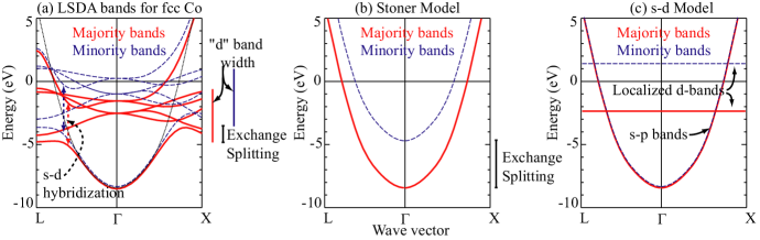
Figure 4: Model band structures for ferromagnets. The solid red (dashed blue) curves give the majority (minority) bands along two high symmetry directions through the Brillouin zone center, $\Gamma$. Panel (a) gives bands calculated in the LSDA for face-centered cubic (fcc) Co. The dotted black curve shows what the energy of the $s$-$p$ band would be if it were not hybridized with the $d$ bands. The bars to the right of (a) show the width of the $d$ bands and the shift between the majority and minority bands. The dashed arrows in (a) indicated the widths of avoided level-crossings due to the hybridization between the $s$-$p$ and $d$ bands of the same symmetry along the chosen direction. Panel (b) gives a schematic version of a Stoner model for a ferromagnet. The exchange splitting is larger than in (a) in order to produce a reasonable size moment. The majority and minority Fermi surfaces are more similar to each other than they are for the LSDA model. Panel (c) gives a schematic s-d model band structure. The current-carrying s-p bands have a very small splitting due to the weak exchange interaction with the localized d-states. The majority and minority Fermi surfaces are almost identical.

The origins of spin-polarized currents in magnetic devices and the giant magnetoresistance (GMR) effect can be understood as consequences of the difference in band structures for the majority-spin and minority-spin states in magnets, as predicted by LSDA calculations and illustrated in a over-simplified way by the exchange splitting in the free-electron Stoner model. Spin-polarized currents can come about because the spin-dependent electron properties in ferromagnets allow magnetic thin films to act like spin filters. Consider the example of Cr/Fe multilayers in which GMR was first discovered. For electrons incident from Cr into a Fe layer, minority spins have a greater probability to be transmitted through the Fe film than majority spins, due to differences scattering caused by the band-structure mismatch at the interface and also due to band-structure-induced differences in the strength of scattering from defects and impurities in the Fe layer [59]. Therefore the current transmitted through the Fe layer in a Cr/Fe/Cr device is partially spin-polarized in the minority direction, while the current reflected from the layer is partially polarized in the majority direction. Many other factors can also affect the ultimate polarization of the currents, including the layer thickness and the spin flip scattering rates.

Once in a non-ferromagnetic metal like Cr or Cu, a spin-polarized current persists on the scale of the spin diffusion length, typically on the order of 100 nm or more in Cu and about 5 nm in Cr. When two Fe layers in a Cr/Fe multilayer are spaced more closely than this and have parallel magnetic moments, minority electrons have a high probability of being transmitted through both layers, resulting in a relatively low overall device resistance even though the majority electrons are scattered strongly. In effect, the minority electrons “short out” the structure, giving a low resistance. When nearby magnetic layers have antiparallel moments, both majority and minority electrons scatter strongly in either one layer or the other, and the resulting resistance is higher. This is the origin of GMR. Other combinations of normal metals and magnetic layers can act similarly, although for combinations like Cu/Co or Cu/Ni it is the majority electrons that are more easily transmitted through the magnetic layer, rather than the minority electrons [59, 60]. A number of different theoretical approaches have been used to calculate the transport properties of magnetic multilayers and their GMR [61, 62, 63]. These techniques will be discussed in more detail in Section 4.

Micromagnetics. In order to describe the equilibrium configuration of the magnetization in a ferromagnet, or the dynamical response to an applied magnetic field or a spin-transfer torque, it can be important to take into account that the magnetization distribution may become spatially non-uniform. Micromagnetics [64, 65, 66] is a phenomenological description of magnetism on a mesoscopic length scale designed to model such non-uniformities in an efficient way. It does not attempt to describe the behavior of the moment associated with each atom, but rather adopts a continuum description much like elasticity theory. Its utility arises because the length scales of interest in magnetic studies are frequently much longer than atomic lengths. Atomic scale calculations become impractical in this case.

In equilibrium, the magnetization direction aligns itself with an effective field, which can vary as a function of position. There are generally four main contributions to this effective field: the externally applied magnetic field, magnetocrystalline anisotropy, micromagnetic exchange, and the magnetostatic field. Each of the fields is most easily described in terms of an associated contribution to the free energy. The total effective field is then the functional derivative of the free energy with respect to the magnetization $\mu_{0}H_{\rm eff}({\bf r})=-\delta E/\delta{\bf M}({\bf r})$. The magnetocrystalline anisotropy arises from the spin-orbit interactions and tends to align the magnetization with particular lattice directions. Generally speaking the anisotropy field is a local function of the magnetization direction and has a different functional form for different lattices and materials. The micromagnetic exchange [67] is the interaction that tends to keep the magnetization aligned in a common direction, adding an energy cost when the magnetization rotates as a function of position. The magnetostatic interaction is a highly non-local interaction between the magnetization at different points mediated by the magnetic field produced by the magnetization. Together, the four free energies can be written

$$E = -\mu_{0}\int d^{3}r{\bf H}_{\rm ext}\cdot{\bf M}({\bf r})-{K_{\rm u}\over M_{\rm s}^{2}}\int d^{3}r(\hat{\bf n}\cdot{\bf M}({\bf r}))^{2}$$

$$+{A_{\rm ex}\over M_{\rm s}^{2}}\int d^{3}r\sum_{\alpha}({\partial\over\partial r_{\alpha}}{\bf M})^{2}$$

$$-{\mu_{0}\over 8\pi}\int d^{3}r\int d^{3}r^{\prime}{\bf M}({\bf r})\cdot{3({\bf M}({\bf r^{\prime}})\cdot{\bf x}){\bf x}-{\bf M}({\bf r^{\prime}})|{\bf x}|^{2}\over|{\bf x}|^{5}},$$

where ${\bf x}={\bf r}-{\bf r}^{\prime}$, $r_{\alpha}=x,y,z$, $M_{\rm s}$ is the saturation magnetization, $A_{\rm ex}$ is the exchange constant, and $K_{\rm u}$ is the anisotropy constant. Here we have taken the specific example of a uniaxial anisotropy with an easy axis along $\hat{\bf n}$. The total effective field derived from Eq. (2) is

$${\bf H}_{\rm eff} = {\bf H}_{\rm ext}+{2K_{\rm u}\over\mu_{0}M_{\rm s}^{2}}\hat{\bf n}(\hat{\bf n}\cdot{\bf M}({\bf r}))+{2A_{\rm ex}\over\mu_{0}M_{\rm s}^{2}}\nabla^{2}{\bf M}$$ (2)

$$+{1\over 4\pi}\int d^{3}r^{\prime}{3({\bf M}({\bf r^{\prime}})\cdot{\bf x}){\bf x}-{\bf M}({\bf r^{\prime}})|{\bf x}|^{2}\over|{\bf x}|^{5}}.$$

The atomic-like exchange, which drives the formation of the magnetization and which is not explicit in these expressions, places a strong energetic penalty on deviations of the magnitude of ${\bf M}({\bf r})$ away from $M_{\rm s}$. This interaction is generally taken into account by treating ${\bf M}({\bf r})$ as having the fixed length $M_{\rm s}$.

Magnetic Domains. The interactions within Eqs. (2) and (2) can compete with one another in determining the orientation of ${\bf M}$ as a function of position. Different interactions can dominate on different spatial scales, with the consequence that the magnetic ground state is often spatially non-uniform, containing non-trivial magnetization patterns even in equilibrium. The micromagnetic exchange and magnetocrystalline anisotropy both represent relatively short-ranged or local interactions. The micromagnetic exchange tends to keep the magnetization spatially uniform and the magnetocrystalline anisotropy can tend to keep it directed in particular lattice directions. For the energy functional above, with uniaxial anisotropy, those directions are $\pm\hat{\bf n}$. For the materials of interest for spin transfer applications the magnetocrystalline anisotropy is frequently weak and does not play an important role (although there are exceptions [68, 69]).

Anisotropies in spin transfer devices are more commonly the result of the sample shape. Magnetostatic interactions favor magnetization orientations aligned in the plane of thin-film samples and along the long axis of samples with non-circular cross-sections. Because of the dipole pattern of long-ranged magnetic fields, the magnetostatic interaction can also favor antiparallel alignment of the magnetization in distant parts of a sample, and this can cause the magnetization pattern to become non-uniform. On short length scales the magnetostatic interaction is relatively weak in comparison to micromagnetic exchange. However the magnetostatic interaction is long-ranged so that it can eventually dominate in large enough samples. This causes the magnetization pattern to depend on the sample size. For magnetic thin-film samples smaller than about 100 nm to 200 nm in diameter, the ground state is approximately (but not exactly) uniform, with the micromagnetic exchange dominating the magnetostatic interactions [70]. For samples slightly bigger than this, magnetostatic interactions become more important and the ground state can be a vortex state. For still larger samples, the magnetization pattern may break up into regions which have different magnetic orientations but within which the magnetization is roughly uniform. These regions are called domains [71].

The border region between domains is referred to as a domain wall. Here the magnetization rotates over a relatively short distance from one domain’s orientation to the other’s. The more gradual is this rotation, the less the cost in exchange energy. However, wider domain walls deviate from the low-energy orientation for magnetocrystalline anisotropy over a larger volume, and therefore cost more anisotropy energy. The domain wall width is determined by a compromise which minimizes the total energy of exchange + anisotropy, and can be characterized roughly by the scale $\ell_{\rm DW}=\sqrt{A_{\rm ex}/K_{\rm u}}$. This length is strongly material dependent, ranging from $\approx$ 1 nm for hard magnetic materials to more than 100 nm for soft magnetic materials. In cases with weak anisotropy, domain wall widths are determined by a competition between exchange and magnetostatic interactions. The domain wall width can also depend on sample geometry, and in a narrow contact between electrodes the wall width can be narrowed in proportion to the contact diameter [72].

In thin-film wires, typical of those used to study current-induced domain wall motion, domain walls typically take one of two structures, “transverse” walls or “vortex” walls. On either side of the wall, the magnetization lies in-plane and points along the length of the wire to minimize the magnetostatic energy, and there is a net 180^∘ rotation of the magnetization at the wall. In a transverse wall, the magnetization simply rotates in the plane of the sample from one domain to the other. However, the competition between the micromagnetic exchange energy and the magnetostatic energy causes the wall width to be narrow (on the scale of the exchange length, $\ell_{\rm ex}=\sqrt{2A_{\rm ex}/(\mu_{0}M_{\rm s}^{2})}\approx$ 4 nm to 8 nm, where $A_{\rm ex}$ is the prefactor of the micromagnetic exchange in Eq. (2) and $M_{\rm s}$ is the saturation magnetization) on one edge of the wire and wide (on the scale of the width of the wire) on the other edge. A vortex wall is even more complicated. Here, the magnetization wraps around a central singularity [73], the vortex core, giving a circulating pattern to the magnetization. The competition between these two wall structures is studied in Ref. [74]. Beach, Tsoi, and Erskine describe how the detailed structure of domain walls plays a crucial role in their motion when they are driven by either an applied magnetic field or a spin transfer torque.

Magnetic Dynamics in the Absence of Spin Transfer Torques. When a magnetic configuration is away from equilibrium, the magnetization precesses around the instantaneous local effective field. In the absence of dissipation, the magnetization distribution stays on a constant energy surface. In order to account for energy loss, Landau and Lifshitz [75] introduced a phenomenological damping term into the equation of motion and Gilbert [76] introduced a slightly different form several decades later. Both forms of the damping move the local magnetization vector toward the local effective field direction:

$${\dot{\bf M}} = -\gamma_{0}^{\prime}{\bf M}\times{\bf H}_{\rm eff}-{\lambda\over M_{s}}{\bf M}\times\left({\bf M}\times{\bf H}_{\rm eff}\right)$$

(Landau-Lifshitz)

$${\dot{\bf M}} = -\gamma_{0}{\bf M}\times{\bf H}_{\rm eff}+{\alpha\over M_{s}}{\bf M}\times{\dot{\bf M}},$$ (3)

(Gilbert)

where $\gamma_{0}$ is the gyromagnetic ratio, $\lambda$ is the Landau-Lifshitz damping parameter, and $\alpha$ is the Gilbert damping parameter. These two forms are known to be equivalent with the substitutions, $\gamma_{0}^{\prime}=\gamma_{0}/(1+\alpha^{2})$ and $\lambda=\gamma_{0}\alpha/(1+\alpha^{2})$. In spite of this equivalence, there has been an ongoing debate about which is more correct. This debate has been rekindled with the interest in current-driven domain wall motion (one of the present authors is guilty of contributing to the debate) and is mentioned in the articles by Tserkovnyak, Brataas, and Bauer and by Berkov and Miltat. Part of the fervor of the debate arises from the fact that it is not experimentally testable. Appropriate equations of motion can be formulated with either form of damping at the expense of slight modifications to other terms in the equation of motion. This point is discussed further in Sec. 5. Note that both the precession and damping terms rotate the magnetization, but do not change its length. This is consistent with treating the magnetization as having a fixed length.

There have been many attempts to compute the damping parameters from models for various physics processes [77]. Some mechanisms are intrinsic to the material, such as those due to magnetoelastic scattering [78], and others are considered extrinsic like two-magnon scattering from inhomogeneities [79]. It appears that a model due to Kambersky [80] for electron-hole pair generation describes the dominant source of intrinsic damping in a variety of metallic systems including the ferromagnetic semiconductors [81] and transition metals [82] primarily of interest for spin transfer torque applications. For a magnetic element in metallic contact with other materials, there can also be a contribution to the damping from “spin-pumping” – the emission of spin-angular momentum from the precessing magnet via the conduction electrons [83, 84, 85].

Magnetization dynamics is most easily investigated using the macrospin approximation. The macrospin approximation assumes that the magnetization of a sample stays spatially uniform throughout its motion and can be treated as a single macroscopic spin. Since the spatial variation of the magnetization is frozen out, exploring the dynamics of magnetic systems is much more tractable using the macrospin approximation than it is using full micromagnetic simulations. The macrospin model makes it easy to explore the phase space of different torque models, and it has been a very useful tool for gaining a zeroth-order understanding of spin-torque physics. However, for many systems of interest, even ones with very small magnetic elements, the macrospin approximation breaks down. For a full understanding of magnetic dynamics, a micromagnetic approach is therefore necessary. The article by Berkov and Miltat discusses some of the circumstances in which the macrospin approach is and is not a reasonable approximation to the true dynamics.

For analyses of magnetic domain wall dynamics, there is a different simplified description that can sometimes be useful for qualitative understanding, as an alternative to full micromagnetic calculations. The Walker ansatz [86] restricts the variation in the domain wall to uniform translations, uniform rotations out of plane, and in some versions a uniform scaling of the wall width. For the simplest version, the dynamics of the domain wall can then be described by two degrees of freedom. The article by Beach, Tsoi and Erskine discusses when this approximation is valid and when it is not for current-induced domain wall motion.

In some situations it is useful to consider the dynamics of a magnetic sample in terms of the normal modes of the system, known as spin waves or magnons, instead of directly integrating the equations of motion at every point on a closely spaced grid designed to model the sample, as is usually done in micromagnetic calculations. A spin wave is a small amplitude oscillation of the magnetization around its average direction. In macroscopic magnetic systems, the spectrum of spin waves is essentially continuous as a function of frequency, but when thin-film magnetic elements are shrunk to the scale of 100 nm in diameter, the spin wave spectrum becomes measurably discrete [87]. In fact, the recent development of spin-transfer-driven ferromagnetic resonance has made it possible to measure the frequencies of these normal modes within individual nanostructures [88, 89]. Interestingly, calculations show that uniform precession, of the type assumed in the macrospin approximation, is generally not a true normal mode because the magnetostatic field is generally not uniform across the sample. An analysis in terms of the normal modes can provide a strategy for simulating magnetic dynamics that is more efficient than standard micromagnetic simulations and somewhat more accurate than the macrospin approximation. The dynamics of a magnetic excitation can be approximated by expanding the excitation using a finite set of normal modes as a basis set, and determining the time dependence based on the dynamics of the individual modes and their nonlinear couplings, rather than by integrating the full equation of motion directly. In cases when the lowest-frequency most-spatially uniform normal mode dominates the magnetic dynamics, the results are typically very similar to the predictions of the simplest macrospin descriptions. The relevance of the spin wave modes is discussed in the articles by Berkov and Miltat and by Sun and Ralph.

3 Spin Current, Spin Transfer Torque, and Magnetic Dynamics

Thus far we have discussed the dynamics of magnets in the absence of the spin transfer torque. Spin transfer torques arise whenever the flow of spin-angular momentum through a sample is not constant, but has sources or sinks. This happens, for example, whenever a spin current (created by spin filtering from one magnetic thin film) is filtered again by another magnetic thin film whose moment is not collinear with the first. In the process of filtering, the second magnet necessarily absorbs a portion of the spin angular momentum that is carried by the electron spins. Changes in the flow of spin angular momentum also occur when spin-polarized electrons pass through a magnetic domain wall or any other spatially non-uniform magnetization distribution. In this process, the spins of the charge carriers rotate to follow the local magnetization, so the spin vector of the angular momentum flow changes as a function of position. In either of these cases, the magnetization of the ferromagnet changes the flow of spin angular momentum by exerting a torque on the flowing spins to reorient them, and therefore the flowing electrons must exert an equal and opposite torque on the ferromagnet. This torque that is applied by non-equilibrium conduction electrons onto a ferromagnet is what we will call the spin transfer torque. Its strength can be calculated either by considering directly the mutual precession of the electron spin and magnetic moment during their interaction (an approach discussed in the article by Haney, Duine, Núñez, and MacDonald) or by considering the net change in the spin current before and after the interaction (the approach we will emphasize).

Our discussion in this Section will consist of two parts. First we will consider how it is that a spin-polarized current can apply a torque to a ferromagnet. This will be straightforward – since a torque is simply a time rate of change of angular momentum, considerations of angular momentum conservation can be used to relate the spin transfer torque directly to the angular momentum lost or gained by spin currents. We will use two simple toy models to illustrate some of the physics involved in this process. The second part of our discussion will describe how to incorporate the spin transfer torque into the equation of motion for the magnetization dynamics. This step of the argument will involve some more-subtle points, related to the connection between the magnetization of a ferromagnet and its total angular momentum. To explore these points fully, we will consider how one might derive the equation of motion for the magnetization, $d{\bf M}/dt$, within a rigorous quantum mechanical theory.

Definition of the Spin Current Density. The primary quantity on which we will focus our interest will be the spin current density ${\bf Q}$. This has both a direction in spin space and a direction of flow in real space, so it is a tensor quantity. For a single electron, the spin current is given classically by the outer product of the average electron velocity and spin density ${\bf Q}={\bf v}\otimes{\bf s}$. For a single-electron wavefunction $\psi$, the spin current density may be written

$${\bf Q} = {\hbar^{2}\over 2m}{\rm Im}(\psi^{*}{\bm{\sigma}}\otimes{\bm{\nabla}}\psi),$$ (4)

where $m$ is the electron mass, and ${\bm{\sigma}}$ represents the Pauli matrices $\sigma_{x}$, $\sigma_{y}$, and $\sigma_{z}$. The form of the spin current density is similar to the more-familiar probability current density $(\hbar/m){\rm Im}(\psi^{*}{\bf\nabla}\psi)$. For a spinor plane-wave wavefunction of the form

$$\psi={e^{ikx}\over\sqrt{{\Omega}}}\left(a\left|\uparrow\right\rangle+b\left|\downarrow\right\rangle\right),$$ (5)

where ${\Omega}$ is a normalization volume, the spatial part of the spin current points in the ${\bf\hat{x}}$ direction, and the three spin components take the simple forms

$$Q_{xx} = {\hbar^{2}k\over 2m{\Omega}}2{\rm Re}(ab^{*})$$

$$Q_{xy} = {\hbar^{2}k\over 2m{\Omega}}2{\rm Im}(ab^{*})$$ (6)

$$Q_{xz} = {\hbar^{2}k\over 2m{\Omega}}(|a|^{2}-|b|^{2}).$$

By conservation of angular momentum, one can say that the spin transfer torque acting on some volume of material can be computed simply by determining the net flux of non-equilibrium spin current through the surfaces of that volume, or equivalently by integrating the divergence of the spin current density within an imaginary pillbox surrounding the volume in question:

$${\bf N}_{\rm st} = -\int_{{\rm pillbox}\ {\rm surfaces}}d^{2}R\hat{\bf n}\cdot{\bf Q}$$ (7)

$$= -\int_{\rm pillbox\ volume}d^{3}r\nabla\cdot{\bf Q},$$

where ${\bf R}$ is the in-plane position and $\hat{\bf n}$ is the interface normal for each surface of the pillbox. (Note that since ${\bf Q}$ is a tensor, its dot product with a vector in real space leaves a vector in spin space.) If one prefers to think in terms of the differential form of Eq. (7), it states that the spin torque density is the divergence of the spin current density.

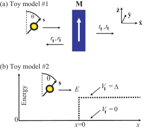
Figure 5: Illustration of toy models discussed in the text.

Toy Model #1. Our first simple model is meant to illustrate that when a spin polarized current interacts with a thin ferromagnetic layer and undergoes spin filtering the result, in general, is that a spin transfer torque is applied to the magnetic layer. Consider the problem of a single-electron state with wave vector ${\bf k}$ in the ${\bf\hat{x}}$ direction and spin oriented in the ${\bf\hat{x}}$-${\bf\hat{z}}$ plane at an angle $\theta$ with respect to the ${\bf\hat{z}}$ direction, which is incident onto a thin magnetic layer whose magnetization is pointed in the ${\bf\hat{z}}$ direction (see Fig. 5(a)). We will initially not be concerned about what goes on inside the magnetic layer, but we will account for its spin filtering properties simply by assuming that it can be described by overall transmission and reflection amplitudes for spin-up electrons ($t_{\uparrow}$, $r_{\uparrow}$) that are different from the transmission and reflection amplitudes for spin-down electrons ($t_{\downarrow}$, $r_{\downarrow}$), and that no spin-flipping processes occur. Under these assumptions, the incident part of the wavefunction is

$$\psi_{\rm in}={e^{ikx}\over\sqrt{{\Omega}}}\Big{(}\cos(\theta/2)\left|\uparrow\right\rangle+\sin(\theta/2)\left|\downarrow\right\rangle\Big{)}.$$ (8)

This can be derived, for example, by starting with the $\left|\uparrow\right\rangle$ state and applying the appropriate rotation matrix for a spin-1/2 system [90]. The transmitted and reflected parts of the scattering wavefunction are

$$\psi_{\rm trans} = {e^{ikx}\over\sqrt{{\Omega}}}\Big{(}t_{\uparrow}\cos(\theta/2)\left|\uparrow\right\rangle+t_{\downarrow}\sin(\theta/2)\left|\downarrow\right\rangle\Big{)}$$

$$\psi_{\rm refl} = {e^{-ikx}\over\sqrt{{\Omega}}}\Big{(}r_{\uparrow}\cos(\theta/2)\left|\uparrow\right\rangle+r_{\downarrow}\sin(\theta/2)\left|\downarrow\right\rangle\Big{)}.$$ (9)

The components of the spin current density can be determined using the expressions given in Eq. (3). The flows of spin density in the ${\bf\hat{x}}$ spatial direction for the incident, transmitted, and reflected parts of the wavefunction take the forms

$${\bf Q}_{\rm in} = {\hbar^{2}k\over 2m{\Omega}}\Big{[}\sin(\theta){\bf\hat{x}}+\cos(\theta){\bf\hat{z}}\Big{]}$$

$${\bf Q}_{\rm trans} = {\hbar^{2}k\over 2m{\Omega}}\sin(\theta){\rm Re}(t_{\uparrow}t_{\downarrow}^{*}){\bf\hat{x}}$$ (10)

$$+{\hbar^{2}k\over 2m{\Omega}}\sin(\theta){\rm Im}(t_{\uparrow}t_{\downarrow}^{*}){\bf\hat{y}}$$

$$+{\hbar^{2}k\over 2m{\Omega}}\Big{[}|t_{\uparrow}|^{2}\cos^{2}(\theta/2)-|t_{\downarrow}|^{2}\sin^{2}(\theta/2)\Big{]}{\bf\hat{z}}$$

$${\bf Q}_{\rm refl} = -{\hbar^{2}k\over 2m{\Omega}}\sin(\theta){\rm Re}(r_{\uparrow}r_{\downarrow}^{*}){\bf\hat{x}}$$

$$-{\hbar^{2}k\over 2m{\Omega}}\sin(\theta){\rm Im}(r_{\uparrow}r_{\downarrow}^{*}){\bf\hat{y}}$$

$$-{\hbar^{2}k\over 2m{\Omega}}\Big{[}|r_{\uparrow}|^{2}\cos^{2}(\theta/2)-|r_{\downarrow}|^{2}\sin^{2}(\theta/2)\Big{]}{\bf\hat{z}}.$$

It is then clear that the total spin current is not conserved during the filtering process: the spin current density flowing on the left of the magnet ${\bf Q}_{\rm in}+{\bf Q}_{\rm refl}$ is not equal to the spin current density on the right ${\bf Q}_{\rm trans}$. By Eq. (7), we can say that the spin transfer torque ${\bf N}_{\rm st}$ on an area $A$ of the ferromagnet is equal to the net spin current transferred from the electron to the ferromagnet, and is given in this toy model by

$${\bf N}_{\rm st} = A{\bf\hat{x}}\cdot({\bf Q}_{\rm in}+{\bf Q}_{\rm refl}-{\bf Q}_{\rm trans})$$ (11)

$$= {A\over\Omega}{\hbar^{2}k\over 2m}\sin(\theta)\Big{[}1-{\rm Re}(t_{\uparrow}t_{\downarrow}^{*}+r_{\uparrow}r_{\downarrow}^{*})\Big{]}{\bf\hat{x}}$$

$$-{A\over\Omega}{\hbar^{2}k\over 2m}\sin(\theta){\rm Im}(t_{\uparrow}t_{\downarrow}^{*}+r_{\uparrow}r_{\downarrow}^{*}){\bf\hat{y}}.$$

We have used the fact that $|t_{\uparrow}|^{2}+|r_{\uparrow}|^{2}=1$ and $|t_{\downarrow}|^{2}+|r_{\downarrow}|^{2}=1$. There is no component of spin torque in the ${\bf\hat{z}}$ direction. We find the general result that the spin transfer torque is zero when $t_{\uparrow}=t_{\downarrow}$ and $r_{\uparrow}=r_{\downarrow}$ (in which case the “magnetic” layer would provide no spin filtering) or when the incoming spin orientation is collinear with the magnetization of the layer, $\theta=0$ or $\pi$. However, for any non-collinear spin orientation, when the magnet does provide spin filtering, it is a direct consequence of the spin filtering that the spin transfer torque acting on the ferromagnetic layer is non-zero. This torque is perpendicular to the magnetization of the layer (no ${\bf\hat{z}}$ component), and for an individual incident electron the torque may have components in both the ${\bf\hat{x}}$ and ${\bf\hat{y}}$ directions, depending on the values of the transmission and reflection coefficients.

It is possible to extend this type of 1-d toy model to calculate the torque applied to a magnetic thin film in a realistic 3-dimensional sample. The calculation proceeds by summing the torque contributed by electron waves incident onto the magnetic thin film from throughout the Fermi surface of the non-magnetic metal, corresponding to electrons incident from many directions in real space [91]. This requires summing the contributions to the ${\bf\hat{x}}$ and ${\bf\hat{y}}$ components of the torque in Eq. (11). In terms of the terminology commonly used in this field [92, 62], the sum over the ${\bf\hat{x}}$-component contributions is proportional to the real part of the “mixing conductance” and gives the “in-plane” torque (the plane defined by the moments on the ferromagnet and the incoming spin), and the sum over the ${\bf\hat{y}}$-component contributions is proportional to the imaginary part of the mixing conductance and gives a perpendicular torque.

Toy Model #2. Next we consider a second simple 1-dimensional toy model [93], to illustrate some of the processes that occur near a normal metal/ferromagnetic interface and influence the spin torque. Here we again first assume a single incoming spin-polarized electron wavefunction of the form given by Eq. (8) incident onto a magnetic layer whose magnetization is in the ${\bf\hat{z}}$ direction. However, in this case we will use a Stoner-model approach to describe the magnetic layer. That is, we will assume that the electrons inside the ferromagnetic layer experience an exchange splitting $\Delta$ which shifts the states in the minority-spin band (down electrons) higher in energy than the majority-spin band (up electrons), but that both bands have a free-electron dispersion. The physics near the interface can then be modeled as a simple scattering problem in which the electron scatters from a rectangular potential-energy step (at position $x=0$) that has different heights for spin-up and spin-down electrons (see Fig. 5(b)). For simplicity, we will assume that the height of the potential-energy step is 0 for up spins and $\Delta$ for down spins, and we will consider an electron energy $E=\hbar^{2}k^{2}/(2m)$ which is greater than $\Delta$.

By matching wavefunctions and their derivatives at the interfaces, it is an elementary problem to calculate the transmitted and reflected parts of the scattering-state wavefunction with energy eigenvalue $E$:

$$\psi_{\rm trans} = {e^{ik_{\uparrow}x}\over\sqrt{{\Omega}}}\cos(\theta/2)\left|\uparrow\right\rangle+{e^{ik_{\downarrow}x}\over\sqrt{{\Omega}}}{2k\over k+k_{\downarrow}}\sin(\theta/2)\left|\downarrow\right\rangle$$

$$\psi_{\rm refl} = {e^{-ikx}\over\sqrt{{\Omega}}}{k-k_{\downarrow}\over k+k_{\downarrow}}\sin(\theta/2)\left|\downarrow\right\rangle,$$ (12)

where $k_{\uparrow}=k$ and $k_{\downarrow}=[2m(E-\Delta)]^{1/2}/\hbar<k$. The incident, transmitted, and reflected spin currents are

$${\bf Q}_{\rm in} = {\hbar^{2}\over 2m{\Omega}}\left(k\sin(\theta){\bf\hat{x}}+k\cos(\theta){\bf\hat{z}}\right)$$

$${\bf Q}_{\rm trans} = {\hbar^{2}\over 2m{\Omega}}\sin(\theta)k\cos[(k_{\uparrow}-k_{\downarrow})x]{\bf\hat{x}}$$

$$-{\hbar^{2}\over 2m{\Omega}}\sin(\theta)k\sin[(k_{\uparrow}-k_{\downarrow})x]{\bf\hat{y}}$$

$$+{\hbar^{2}\over 2m{\Omega}}\left[k\cos^{2}(\theta/2)-k_{\downarrow}\left({2k\over k+k_{\downarrow}}\right)^{2}\sin^{2}(\theta/2)\right]{\bf\hat{z}}$$

$${\bf Q}_{\rm refl} = {\hbar^{2}\over 2m{\Omega}}k\left({k-k_{\downarrow}\over k+k_{\downarrow}}\right)^{2}\sin^{2}(\theta/2){\bf\hat{z}}.$$

There are two points of physics that we wish to illustrate with this example. First, the transverse (perpendicular to ${\bf\hat{z}}$) spin component of the reflected spin current density is equal to zero. Since the total spin current density is continuous at the interface, this means that all of the of the transverse component of the incident spin current density is transmitted through the interface; none is reflected. In this toy model, this result follows from our assumption that for spin up electrons the height of the potential-energy step at the interface is zero, so that the reflection amplitude for spin up electrons is zero and the reflected part of the wavefunction is purely spin down. For models in which both components of spin experience a non-zero potential-energy step, some of the incident ${\bf\hat{x}}$ component of the spin current density will be reflected. However, for many of the materials combinations used commonly in metallic GMR devices, like Cu/Co, Cu/Ni, or Cr/Fe, one of the spin components actually does have a reflection amplitude close to zero over a large part of the Fermi surface [94, 95, 93], so it is a reasonable approximation in these cases that almost all of the transverse (${\bf\hat{x}}$) component of the spin current density will be transmitted into the ferromagnet.

The second important point of physics illustrated by the model concerns what happens to the transverse component of the spin current density after it enters the ferromagnet. The oscillatory ${\bf\hat{x}}$ and ${\bf\hat{y}}$ terms in the transmitted spin current density represent precession of the spin about the ${\bf\hat{z}}$ axis as a function of position as it penetrates through the magnet. In any model in which there is a difference in exchange energy between majority and minority spin states, the two spin components of a wavefunction for a given eigenvalue $E$ must have different kinetic energies, so that $k_{\uparrow}\neq k_{\downarrow}$ and the spin state inside the magnet will precess. The same phenomenon is therefore present in more rigorous models. One can view this effect as simply the precession of the spin in the exchange field of the magnet. The period of the precession, $2\pi/(k_{\uparrow}-k_{\downarrow})$ is very short for a typical transition metal ferromagnet, on the scale of a few atomic lattice spacings. This is important because in real 3-dimensional samples many electrons are incident on the magnetic layer from a variety of directions, corresponding to states from all parts of the Fermi surface, and therefore different electrons take different paths through the magnetic layer. Even if all of the electrons begin with perfectly aligned spins at the normal-metal/ferromagnet interface, electrons reaching a given depth inside the magnet will have traveled different path lengths to get there. The result is classical dephasing. Electron spins that have traveled different path lengths will have precessed by different angles around the ${\bf\hat{z}}$ direction, and therefore their ${\bf\hat{x}}$ and ${\bf\hat{y}}$ components will not add constructively. For locations more than a few atomic lattice constants into a magnetic layer, when one sums over electrons from all relevant parts of the Fermi surface in calculations that include first-principles computations of the transmission amplitudes [95, 93, 96], the transverse (to ${\bf\hat{z}}$) components of the spins average to zero. As a consequence of this classical dephasing, there is no net transmission of transverse spin angular momentum through the ferromagnet. The transverse angular momentum that enters into the ferromagnet is effectively absorbed within a few atomic layers from the interface.

For a full calculation of the spin torque at an interface in a real 3-dimensional sample, it is important to take into account not just propagating wavefunctions, but also evanescent scattering states at the interface. If our toy model #2 is generalized to three dimensions, evanescent scattering wavefunctions are required in cases where the incident electron approaches the interface from a glancing angle, so that the part of the kinetic energy associated with the perpendicular wavevector is less than the step height $\Delta$. In calculations with more realistic band structures, both evanescent and propagating scattering states can couple to incident Bloch states more generally, and it is necessary to take the evanescent states into account to guarantee the continuity of the wavefunction and its first derivative on the atomic scale. Although evanescent scattering states do not carry charge current, they do carry spin current, so that they can contribute a significant spin torque even when the net charge flow through the interface is zero. This point can be illustrated by our toy model if we consider a case in which the spin-dependent step heights are sufficiently high that both of the spin components are completely reflected. The transmitted and reflected parts of the scattering wavefunction are then

$$\psi_{\rm trans} = {e^{-\kappa_{\uparrow}x}\over\sqrt{{\Omega}}}\frac{2k}{k+i\kappa_{\uparrow}}\cos(\theta/2)\left|\uparrow\right\rangle$$

$$+{e^{-\kappa_{\downarrow}x}\over\sqrt{{\Omega}}}\frac{2k}{k+i\kappa_{\downarrow}}\sin(\theta/2)\left|\downarrow\right\rangle,$$

$$\psi_{\rm refl} = {e^{-ikx}\over\sqrt{{\Omega}}}\frac{k-i\kappa_{\uparrow}}{k+i\kappa_{\uparrow}}\cos(\theta/2)\left|\uparrow\right\rangle$$ (14)

$$+{e^{-ikx}\over\sqrt{{\Omega}}}\frac{k-i\kappa_{\downarrow}}{k+i\kappa_{\downarrow}}\sin(\theta/2)\left|\downarrow\right\rangle,$$

where $\kappa_{\uparrow}$ and $\kappa_{\downarrow}$ are decay constants for the evanescent states in the ferromagnet. Because the transmission and reflection amplitudes are now complex, with (in general) different complex phases for spin up and spin down electrons, the transmitted and reflected spin current densities will contain ${\bf\hat{y}}$ as well as ${\bf\hat{x}}$ components. The transmitted spin current density also decays exponentially to zero as a function of the penetration distance into the ferromagnet. What this means is that, in effect, the electron penetrates into the ferromagnet a distance on the order of $1/(\kappa_{\uparrow}+\kappa_{\downarrow})$ and precesses around the exchange field as it does so, so that when it emerges from the magnet it is rotated away from its original orientation. Consequently, during the process of reflection an electron can apply a torque to the magnet in both the in-plane and perpendicular directions.

In calculations with realistic band structures for normal-metal/ferromagnet interfaces, when one sums over the Fermi surface to determine the total value of the transverse part of the reflected spin current there is significant (but not perfect) classical dephasing, so that the overall net flow of reflected transverse angular momentum is close to zero [93, 95, 96]. This means that the incident transverse angular momentum that couples into the evanescent states cannot end up flowing away from the interface through the reflected states. Instead, this transverse spin angular momentum is deposited in the interfacial region of the ferromagnet via the torque from the evanescent states. This contribution to the torque, which is not directly mediated by the propagating states, can be described as due to spin filtering. If one accounts for the evanescent states when constructing the scattering states but then ignores their contribution to the spin current, the spin-filtering contribution corresponds to the resulting interfacial discontinuity in the part of the spin current density carried by just the propagating states.

The net result of the classical dephasing that occurs for both transmitted and reflected electron waves at a normal-metal/ferromagnet interface is that the total transmitted and reflected spin currents, summed over all relevant states on the Fermi surface, are approximately collinear with the ferromagnetic layer’s magnetization (in the ${\bf\hat{z}}$ direction, in our toy model). Since, to a good approximation, no transverse angular momentum flows away from the magnet, this collinearity means that approximately the entire incident transverse spin current is absorbed near the normal-metal/ferromagnet interface, and the spin transfer torque (Eq. (7)) becomes

$${\bf N}_{\rm st} = A{\bf\hat{x}}\cdot({\bf Q}_{\rm in}+{\bf Q}_{\rm refl}-{\bf Q}_{\rm trans})\approx A\hat{\bf x}\cdot{\bf Q}_{{\rm in}\perp}.$$ (15)

In terms of the parameters used in our first toy model above, it is correct to say that when summing or averaging over all contributions from around the Fermi surface that to a good approximation for a typical metallic interface the dephasing leads to $\langle{\rm Re}(t_{\uparrow}t_{\downarrow}^{*})\rangle=\langle{\rm Im}(t_{\uparrow}t_{\downarrow}^{*})\rangle=\langle{\rm Im}(r_{\uparrow}r_{\downarrow}^{*})\rangle=0$, and to a somewhat less-accurate approximation $\langle{\rm Re}(r_{\uparrow}r_{\downarrow}^{*})\rangle\approx 0$, so that on average for our one electron

$${\bf N}_{\rm st}\approx{A\over{\Omega}}{\hbar^{2}k\over 2m}\sin(\theta){\bf\hat{x}},$$ (16)

and the spin torque acting on the magnet per unit area is equal to the full component of incident spin current that is transverse to the ferromagnet’s moment.

The result in Eq. (15) is a good approximation for metallic interfaces, like Cr/Fe or Cu/Co, but the processes that lead to the simple form $A\hat{\bf x}\cdot{\bf Q}_{{\rm in}\perp}$ may be different for magnetic semiconductors or for tunnel junctions like Fe/MgO/Fe. Most electrons that scatter from tunnel barriers reflect, whether they are majority or minority. In addition, tunneling is dominated by electrons that are largely from particular parts of the Fermi surface, so the classical dephasing processes that are important for metallic junctions may be weaker in tunnel junctions. In fact, there is good evidence that $\langle{\rm Im}(r_{\uparrow}r_{\downarrow}^{*})\rangle\neq 0$ in tunnel junctions, so that for large applied biases there can be a significant spin torque component in the ${\bf\hat{y}}$ direction (perpendicular to the plane defined by the incoming electron spin and the ferromagnet’s moment) [97, 98]. This is discussed in more detail in the article by Sun and Ralph.

Before moving on to consider how the spin torque will affect the ferromagnet’s magnetization orientation, we wish to re-emphasize one last important point. Spin currents can flow within parts of devices even where there is no net charge current. Consequently, a spin transfer torque can also be applied to magnetic elements that do not carry any charge current [24, 95]. We have already noted two examples of this effect, in Slonczewski’s original calculation of interlayer exchange coupling in a magnetic tunnel junction [21] and in our toy model #2 for the case when both spin-up and spin-down components of the wavefunction are completely reflected. Another important example occurs in multiterminal normal-metal/ferromagnet devices, which are designed so that a charge current flows only between two selected terminals, but diffusive spin currents may also flow throughout the rest of the device. The groups of Johnson, van Wees, and others have demonstrated non-local spin accumulation in nonmagnetic wires using multiterminal devices [99, 100, 101, 102]. Kimura et al. have used a similar lateral device design to demonstrate spin-torque-driven switching of a thin-film magnetic element which carries no charge current [103]. One can view this effect as due simply to a flow of spin-polarized electrons penetrating by diffusive motion into a magnetic element and transferring their transverse component of spin angular momentum, while an equal number of electrons exit the magnet with an average spin component collinear with the magnet so that they give no spin torque. In this way there can be a non-zero net spin current and therefore a non-zero spin torque on the magnet, even when there is no net charge current. Thus far the switching currents required in the devices of Kimura et al. are larger than those needed to switch comparable magnetic elements in standard magnetic-multilayer pillar devices, because the magnitude of the spin current densities achieved in the lateral devices (per unit injected charge current) is smaller than in the multilayers.

Spin Transfer Torque and the Landau-Lifshitz-Gilbert Equation. To calculate the effects of the spin transfer torque on magnetic dynamics, in practice a term ${\dot{\bf M}}_{\rm st}\propto{\bf N}_{\rm st}$ is generally simply inserted as an additional contribution on the right side of the Landau-Lifshitz-Gilbert equation (Eq. (2)). However, this step deserves some careful consideration, as it involves a few subtle points of physics. First, this insertion assumes that the all of the angular momentum transferred from the transverse spin current density acts entirely to reorient the orientation of the ferromagnet rather than, for example, being absorbed in the excitation of short-wavelength magnon modes or being transferred directly to the atomic lattice. This seems to be a reasonable approximation for describing the experiments performed to date; however, as we note below, the existing spin-torque measurements in metallic multilayer samples are not particularly quantitative.

A second simple matter to keep straight is the sign of the torque. An electron’s magnetic moment is opposite to its spin angular momentum $\bm{\mu}=g_{e}\mu_{\rm B}{\bf S}/\hbar$, where ${\bf S}$ is the total spin and $g_{e}\approx-2.0023$, and likewise in transition metal ferromagnets the magnetization is generally opposite to the spin density ${\bf M}=g\mu_{\rm B}{\bf s}/\hbar$, where ${\bf s}$ is here the spin density and $g$ is typically in the range -2.1 to -2.2 [104]. We have defined ${\bf N}_{\rm st}$ as a time rate of change of angular momentum. Since the Landau-Lifshitz-Gilbert equation is stated in terms of magnetization, the contribution of the spin transfer torque should enter this equation with a sign opposite to the change in angular momentum. In the end, the sign of the spin transfer torque is such as to rotate the spin angular momentum density of the ferromagnet toward the direction of the spin of the incoming electrons, or equivalently to rotate the magnetization of the ferromagnet toward the direction of the moment of the incoming electrons.

A third, potentially much more consequential, subtlety involves the orbital contribution to the magnetization. If we assume that all of the angular momentum in the ferromagnet is due to its spin density, then conservation of angular momentum implies that the effect of spin transfer torque on the magnetization can be described simply by inserting

$${\dot{\bf M}}_{\rm st}=-{\bf N}_{\rm st}|g|\mu_{\rm B}/(\hbar\mathcal{V})$$ (17)

into the right side of the Landau-Lifshitz-Gilbert equation (Eq. (2)). Here $\mathcal{V}$ is the volume of the ferromagnet (free layer) over which the spin torque ${\bf N}_{\rm st}$ is applied. Ignoring any orbital contribution is a reasonable first-order approximation, because the orbital moments in transition metal ferromagnets are largely quenched by the strong hybridization of the d electrons. However, spin-orbit coupling does give rise to a weak orbital moment, typically less than a tenth of the spin moment as indicated by the deviation of $g$ from -2. In a more precise treatment that takes the orbital contribution into account, the total angular momentum density would be ${\bf s}+\bm{\ell}$, and the magnetization would be ${\bf M}=-\mu_{\rm B}(|g_{e}|{\bf s}+\bm{\ell})/\hbar$, so that there might not be any simple proportionality between the total angular momentum density and ${\bf M}$. This would necessitate a significantly more complicated picture, as described in more detail immediately below. However, in most analyses of spin transfer torques, the potential effects of orbital moments are ignored, and it is assumed that the spin torque is simply described by Eq. (17). The appropriateness of neglecting orbital angular momentum is discussed briefly in the article by Haney, Duine, Núñez, and MacDonald.

A More Rigorous Approach to the Equation of Motion for Magnetization. In this section we will discuss how one might take a more systematic approach to deriving the equation of motion for a ferromagnet under the influence of a spin transfer torque. This exercise will give additional insights into what might be required to account more accurately for effects like orbital angular momentum and spin-orbit coupling. This approach also provides a more natural framework for considering spin transfer torques at domain walls and in other spatially non-uniform magnetization distributions.

Our starting point is that the equation of motion for any variable in quantum mechanics can be determined by taking the commutator of the operator corresponding to that variable with the Hamiltonian and then evaluating the expectation value of the result. To explore how this process works, we will consider first the charge density, then the spin density, and finally (briefly) the magnetization. In second quantized notation [105] the charge density and spin density operators are

$$\hat{n} = (-e)\sum_{\sigma}\hat{\psi}^{\dagger}_{\sigma}({\bf r})\hat{\psi}_{\sigma}({\bf r}),$$

$$\hat{{\bf s}} = {\hbar\over 2}\sum_{\sigma,\sigma^{\prime}}\hat{\psi}^{\dagger}_{\sigma}({\bf r})\bm{\sigma}_{\sigma,\sigma^{\prime}}\hat{\psi}_{\sigma^{\prime}}({\bf r}),$$ (18)

in terms of the creation $\hat{\psi}^{\dagger}_{\sigma}$ and destruction $\hat{\psi}_{\sigma}$ operators for an electron at point ${\bf r}$ and spin $\sigma$. These fermion operators obey the anti-commutation relations $\{\hat{\psi}_{\sigma}({\bf r}),\hat{\psi}^{\dagger}_{\sigma^{\prime}}({\bf r}^{\prime})\}=\delta({\bf r}-{\bf r}^{\prime})\delta_{\sigma,\sigma^{\prime}}$. For the present purposes we consider the Hamiltonian for non-interacting electrons as in the mean field LSDA approach

$$\hat{{\mathcal{H}}} = {\hbar^{2}\over 2m}\sum_{\sigma}\int d^{3}r\bm{\nabla}\hat{\psi}^{\dagger}_{\sigma}({\bf r})\cdot\bm{\nabla}\hat{\psi}_{\sigma}({\bf r})$$ (19)

$$+\int d^{3}r\left[V({\bf r})\hat{n}({\bf r})+{2\mu_{\rm B}\over\hbar}{\bf B}_{\rm xc}\cdot\hat{{\bf s}}\right]$$

$$+\int d^{3}r\mu_{0}{g\mu_{\rm B}\over\hbar}({\bf H}_{\rm ext}+{\bf H}_{\rm dip})\cdot\hat{{\bf s}}.$$

The first term in the above equation is the kinetic energy, the second term is the potential, including the local exchange field, and the third term is the coupling with the applied field ${\bf H}_{\rm ext}$ and the dipolar field ${\bf H}_{\rm dip}$ due to the rest of the spins. More generally, the potential, the local exchange field, and the dipolar field are many-body terms, but for the present example they are treated as effective single particle interactions. For the moment we are also ignoring spin-orbit coupling in this Hamiltonian.

Let us first derive the equation of motion for the electron charge density. The only term in the Hamiltonian that does not commute with the charge density operator is the kinetic energy and it gives rise to a term that is the divergence of the charge current density

$${d\hat{n}\over dt} = {1\over i\hbar}[\hat{n},{\mathcal{H}}]$$ (20)

$$= {-e\hbar\over 2im}\sum_{\sigma}\int d^{3}r\bigg{\{}\hat{\psi}^{\dagger}_{\sigma^{\prime}}({\bf r}^{\prime})[\bm{\nabla}_{{\bf r}^{\prime}}\delta(({\bf r}-{\bf r}^{\prime}))]\delta_{\sigma,\sigma^{\prime}}\bm{\nabla}\hat{\psi}_{\sigma}({\bf r})$$

$$-\bm{\nabla}\hat{\psi}^{\dagger}_{\sigma}({\bf r})[\bm{\nabla}\delta(({\bf r}-{\bf r}^{\prime}))]\delta_{\sigma,\sigma^{\prime}}\hat{\psi}_{\sigma^{\prime}}({\bf r}^{\prime})\bigg{\}}$$

$$= -\bm{\nabla}\cdot\hat{\bf j}.$$

The charge current density operator is

$$\hat{\bf j} = {-e\hbar\over 2im}\sum_{\sigma}\left[\hat{\psi}^{\dagger}_{\sigma}({\bf r})\bm{\nabla}\hat{\psi}_{\sigma}({\bf r})-\bm{\nabla}\hat{\psi}^{\dagger}_{\sigma}({\bf r})\hat{\psi}_{\sigma}({\bf r})\right].$$ (21)

Taking the expectation value of Eq. (20) gives simply the continuity equation for the charge density, as is required by charge conservation. The time rate of change of the charge density in some volume is given by the net flux of electrons into that volume.

Finding the time evolution of the spin density can be done using the same method, but this exercise is somewhat more complicated because the spin density is a vector and there are additional terms in the Hamiltonian beside the kinetic energy with which it does not commute. If we ignore spin-orbit coupling we get

$${d\hat{\bf s}\over dt} = -\bm{\nabla}\cdot\hat{\bf Q}-\gamma_{0}\hat{\bf s}\times({\bf H}_{\rm ext}+{\bf H}_{\rm dip}),$$ (22)

where $\hat{\bf Q}$ is the tensor spin current density operator

$$\hat{\bf Q} = {\hbar^{2}\over 4im}\sum_{\sigma,\sigma^{\prime}}\bigg{[}\hat{\psi}^{\dagger}_{\sigma}({\bf r})\bm{\sigma}_{\sigma,\sigma^{\prime}}\otimes\bm{\nabla}\hat{\psi}_{\sigma^{\prime}}({\bf r})$$ (23)

$$-\bm{\nabla}\hat{\psi}^{\dagger}_{\sigma}({\bf r})\otimes\bm{\sigma}_{\sigma,\sigma^{\prime}}\hat{\psi}_{\sigma^{\prime}}({\bf r})\bigg{]},$$

and the dot product in Eq. (22) connects to the spatial index of the spin current. Similar to the contribution in the continuity equation, there is a contribution to the time rate of change in the spin density due to the net flux of spins in and out of a volume (the term involving $\hat{\bf Q}$). In addition, the spin density precesses in the local fields ${\bf H}_{\rm ext}+{\bf H}_{\rm dip}$. There is no contribution from the local exchange field because (at least in the LSDA mean field theory) it is exactly aligned with the expectation value of the local spin density. The cross product between these two quantities is then identically zero.

Comparing Eq. (22) to Eqs. (2) and (2), the astute reader will notice some differences. Eq. (22) does not include a contribution from the magnetocrystalline anisotropy, but this is just because for the present we are ignoring the spin-orbit coupling. More importantly, Eq. (22) appears not to include any term to account for micromagnetic exchange. The explanation for this is that there are actually two contributions to the spin current density ${\bf Q}$ and its divergence within a ferromagnet having a spatially non-uniform magnetization. The first is the non-equilibrium spin current that flows with an applied bias and which is the contribution of interest in this series of articles. A second contribution is present in the absence of any applied bias whenever the magnetization is non-collinear. This contribution can be viewed as the mediator of the micromagnetic exchange interaction in analogy to Slonczewski’s calculation [21] of the exchange coupling across a tunnel barrier. In general in the discussion of spin transfer torques, and in particular in the rest of this article and the accompanying articles, this contribution is taken into account by including explicitly in the equation of motion a micromagnetic exchange contribution in the form $-\bm{\nabla}\cdot{\bf Q}_{\rm eq}=-\gamma_{0}[A_{\rm ex}/(2\mu_{0}M_{\rm s}^{2})]{\bf s}\times\nabla^{2}{\bf M}$, so that the spin current contribution then describes only the non-equilibrium component.

We expect that the equations of motion become even more interesting if one were to include spin-orbit coupling in the Hamiltonian. First, there are additional terms in the equation of motion of the spin density, Eq. (22), because the contribution of spin-orbit coupling to the Hamiltonian will not commute with the spin density operator. One new term generated by the spin-orbit coupling is straightforward: the magnetocrystalline anisotropy gives a contribution $-\gamma_{0}{\bf\hat{s}}\times{\bf H}_{\rm ani}$. The damping term in Eq. (2) emerges as well, when a coupling to a source of energy and angular momentum is also included. The article by Tserkovnyak, Brataas, and Bauer describes the derivation of such terms. However, when the orbital angular momentum in a ferromagnet is appreciable, one should recognize that the quantity of primary interest in the Landau-Lifshitz-Gilbert equation is the magnetization rather than the spin density, and these quantities need no longer be simply proportional to each other. The magnetization operator is $\hat{\bf M}=-\mu_{\rm B}(|g_{e}|{\bf\hat{s}}+{\bf\hat{\ell}})/\hbar$, where ${\bf\hat{\ell}}$ is the orbital angular momentum density operator. When taking the commutator of $\hat{\bf M}$ with the Hamiltonian, the spin part of the magnetization will generate the same divergence of the spin current written in Eq. (22) but there will be a large number of additional terms due to spin-orbit coupling and ${\bf\hat{\ell}}$.

These complications due to spin-orbit coupling are likely to play an important role in the dynamics of ferromagnetic semiconductors discussed in the article by Ohno and Dietl, because spin-orbit coupling is much more significant in these materials than in transition metal ferromagnets. As the spin-orbit coupling is comparable to the exchange splitting in the ferromagnetic semiconductors, the band structure does not divide cleanly into majority and minority bands. This leads to additional complications in calculating transport properties [106], even beyond the complications discussed above. In these materials, it is not even clear that the spin current is the most appropriate current to consider. This question is related to the issues of interest in the study of the spin Hall effect, see [107] for a review. Complications from spin-orbit coupling are also likely to be amplified in ferrimagnetic samples as discussed in the articles by Haney, Duine, Núñez, and MacDonald and by Sun and Ralph.

4 Multilayers and Tunnel Junctions

Device Geometries. For understanding the behavior of spin-torque devices, the simplest geometry to consider consists of two magnetic layers separated by a thin non-magnetic spacer layer. One magnetic layer serves to spin-polarize a current flowing perpendicular to the layer interface (this spin filtering can occur either in transmission or reflection), and then this spin-polarized current can transfer angular momentum to the other magnetic layer to excite magnetic dynamics. The spacer layer can either be a non-magnetic metal or a tunnel junction. In order that magnetic dynamics are excited in one magnetic layer but not both, typically devices are designed to hold the magnetization in one magnetic layer (the “fixed” or “pinned” layer) approximately stationary at least for low currents. This is done either by making this layer much thicker than the other, so that it is more difficult to excite by spin torque, or by fabricating it in contact with an antiferromagnetic layer, which produces an effective field (“exchange bias”) and increases the damping, which both act to keep the ferromagnetic layer pinned in place. The strength of the spin torque acting on the thin “free layer” can be increased by sandwiching it between two different pinned magnetic layers (with moments oriented antiparallel), so that a spin-polarized current is incident onto the free layer from both sides, [108, 109, 110, 111, 112].

Spin transfer devices must be fabricated with relatively small lateral cross sections, less than about 250 nm in diameter for typical materials, in order that the spin torque effect dominates over the Oersted field produced by the flowing current [113]. (The Oersted field is often not negligible even in samples for which the spin torque effect dominates – it can be included in micromagnetic simulations of the magnetic dynamics as an additional contribution to ${\bf H}_{\rm eff}$ in the Landau-Lifshitz-Gilbert equation as described in the article by Berkov and Miltat.) Small device sizes are also convenient for understanding spin-torque-generated magnetic dynamics because the macrospin approximation can become a reasonable approximation, and of course small devices are desired for many applications.

Two general experimental approaches are used to direct current flow through an area $\leq 250$ nm wide in a magnetic multilayer. One is to make electrical contact to an extended multilayer substrate in a “point contact” geometry, made either mechanically with a very sharp tip [25] or using lithography techniques [27, 114]. The other approach is to make “nanopillar” devices in which at least the free magnetic layer and sometimes both the free and the fixed magnetic layers are patterned to a desired cross section. See Fig. 6 for a schematic illustration of both geometries. Nanopillars can be made by electron-beam lithography and ion milling [28], stencil techniques [115], or electrodeposition of layers inside cylindrical nanopores [116]. Samples in which the free layer is patterned but the fixed layer is left as an extended film are convenient for some experiments because this geometry minimizes the magnetostatic coupling between the magnetic layers. In general, point contact devices require much more current density to excite magnetic dynamics with spin torque, because the excitations must reorient a small region in an extended magnetic film, working against strong micromagnetic exchange. Typical critical current densities for excitations in point contact devices are $10^{8}$ A/cm² to $10^{9}$ A/cm², while nanopillar devices have achieved current densities of $<10^{7}$ A/cm². As far as we are aware, the record low intrinsic (extrapolated to $T=0$) critical current in a nanopillar device with a magnetic free layer that is thermally stable at room temperature is 1.1 $\times$ 10⁶ A/cm² [117]. Two of the nice features of nanopillars are that they can be made to have two different stable magnetic configurations at zero applied magnetic field for memory applications, and recently they have enabled direct x ray imaging of current-driven magnetic dynamics [118]. Point contacts have an advantage in that they give narrower linewidths ($\Delta f/f$) as a function of frequency $f$ when used to make spin-transfer nano-oscillators, as described below. Both point contacts [27, 119, 120] and nanopillars [121] have also been used to study samples with a single ferromagnetic layer. The article by Katine and Fullerton describes some of the strategies which can be employed to decrease the critical current density for magnetic switching in nanopillars. The article by Silva and Rippard discusses research on point contact devices.

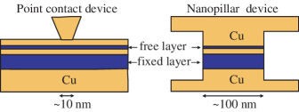
Figure 6: Schematic experimental geometries.

Methods for Calculating Spin Torques. From a theoretical point of view, a consensus has developed [62, 63, 122] for the general approach to be used for calculating spin torques in metal multilayers. We note however, that there is not universal agreement that this model is correct [123, 124, 125]. To solve for the spin transfer torque acting on a static magnetic configuration, the consensus view is that one should determine the spin current density ${\bf Q}$ through an analysis of the spin-dependent electron transport in the device structure, and then identify the torque from the divergences of ${\bf Q}$ near magnetic interfaces or in regions of non-uniform magnetization. (As we noted above, this assumes that no angular momentum is lost to the excitation of short-wavelength spin wave modes or to other processes.)

To calculate the spin torque on a moving magnetic configuration, a somewhat more sophisticated procedure is in principle necessary, for a rigorous treatment, in order to take into account the “spin-pumping” effect [83]. Spin pumping refers to the fact that a precessing magnetization can produce a non-zero spin current density in a magnetic device, in addition to the spin current density generated directly by any applied bias. The total spin torque on the moving magnetization should be determined from the divergence of the total spin current arising from both sources. However, typically the primary effect of spin pumping is merely to increase the effective damping of the ferromagnet in a way that is independent of bias (although it may depend strongly on the precession angle [126]), so that spin pumping can be taken into account approximately just by renormalizing the damping constant. Then the spin transfer torque even on a moving magnetization configuration can be determined, approximately, from the divergence of just the bias-dependent part of the spin current density.

Once the spin torque is calculated, the response of the magnetization is generally determined by inserting this torque as an additional contribution to the classical Landau-Lifshitz Gilbert equation of motion (Eq. (2)). The article by Haney, Duine, Núñez, and MacDonald describes this consensus approach as the “bookkeeping theory.” Spin pumping can also be incorporated into fully self-consistent solutions without too much extra difficulty, because spin pumping is local in time, depending only on ${\bf M}$ and ${\dot{\bf M}}$, and it can be calculated within the same type of theoretical framework needed for calculating the direct bias-generated spin torque [126, 127].

Depending on the amount of disorder in the device and other details, there are a number of strategies for computing the spin current density, some of which are compared in Ref. [128]. If scattering within a layer is weak enough that most electrons do not scatter except at interfaces, the transport is called ballistic. The opposite limit, in which most electrons scatter several times while traversing a layer, is called diffusive. Calculations for particular devices can be complicated by the fact that some layers may be in the diffusive limit while others are in the ballistic limit and some layers are in between.

The ballistic regime can be treated by constructing the scattering states of the system [91, 96], by the Keldysh formalism [129] or by non-equilibrium Green’s functions [130]. References [129] and [130] have considered some of the potential effects of quantum coherence in the ballistic limit, but these effects are generally not expected to be important in the types of metallic multilayer samples typically studied experimentally, because their interfaces are not sufficiently abrupt and perfect. In principle, scattering-state formalisms, the Keldysh method, and non-equilibrium Green’s functions techniques can all be extended into the diffusive regime, but the strong scattering in the diffusive regime is generally easier to treat using the semiclassical approaches discussed next.

The Boltzmann equation [131, 132] neglects coherent effects, but is accurate for both ballistic and diffusive samples, and can interpolate between these limits. In the Boltzmann-equation approach, the transport is described in terms of a semiclassical distribution function so that the behavior of electrons on different parts of the Fermi surface are tracked separately. Other calculation strategies are based on approximations that sum over this distribution function and compute the transport in terms of just its moments. These include the drift-diffusion approximation [133, 134, 135] and circuit theory [92]. For the non-collinear magnetic configurations considered here, these approximations are extensions of Valet-Fert theory [61], which is widely used to describe GMR for collinear magnetizations.

In all of these approaches, the transport across the interfaces is described in terms of spin-dependent transmission and reflection amplitudes. For electron spins that are collinear with the magnetization, these processes are incorporated into the transport calculations as boundary conditions between the solutions of the transport equations in each layer, and the results are spin-dependent interface resistances [136] (or conductances). For spins that are not collinear, transmission and reflection give rise both to boundary conditions on the transport calculations and also give the spin transfer torque. In the drift-diffusion approach, the non-collinear boundary conditions are that the transverse spin current is proportional to the transverse spin accumulation

$${\bf Q}_{\perp}^{\rm NM}\cdot\hat{\bf n}=w{\bf m}_{\perp}^{\rm NM},$$ (24)

where $\hat{\bf n}$ is the interface normal, $w$ is a characteristic velocity, ${\bf m}_{\perp}^{\rm NM}$ is the transverse spin accumulation, and the ${\rm NM}$ superscript indicates that the transverse spin density and spin current are evaluated in the non-magnet as they are both zero in the ferromagnet. This boundary condition has a straightforward interpretation. Since the interface acts as an absorber of any transverse spin component that scatters from it, there is no out-going spin current to cancel the incoming spin current, so there must be a net accumulation of transverse spins in the non-magnet near the interface. Since the incident transverse spin current is equal to the spin transfer torque it is also the case that the transverse spin accumulation is proportional to the spin transfer torque. The relation leads some authors to discuss separate spin current and spin accumulation mechanisms for the spin transfer torque. However, from this discussion, we see that the two are intimately related, and the spin transfer torque can be fully accounted for in terms of the spin current; there is not an extra separate contribution from spin accumulation.

For the case of a symmetric two-magnetic-layer device with a metal spacer, Slonczewski [137] calculated the spin transfer torque using a simplified Boltzmann equation grafted with circuit theory. He found that the torque on the free layer magnetization ${\bf M}$ due to the misalignment with fixed layer magnetization ${\bf M}_{\rm fixed}$ can be described by adding to the Landau-Lifshitz-Gilbert equation (Eq. (2)) a term of the form

$${\dot{\bf M}}_{\rm st}=\eta(\theta){\mu_{\rm B}I\over e\mathcal{V}}~{}\hat{\bf M}\times(\hat{\bf M}\times\hat{\bf M}_{\rm fixed}),$$ (25)

where $I$ is the current, $\mathcal{V}$ is the free-layer volume on which the spin torque acts, $\eta(\theta)={q/(A+B\cos\theta)}$, $\hat{\bf M}$ and $\hat{\bf M}_{\rm fixed}$ are unit vectors in the directions of ${\bf M}$ and ${\bf M}_{\rm fixed}$ (not operators), and $\cos\theta=\hat{\bf M}\cdot\hat{\bf M}_{\rm fixed}$. All of the details of the layer structure are buried in the constants $q$, $A$, and $B$. Very similar results have also been found by a variety of other theoretical approaches. Below, we will sometimes refer loosely to ${\dot{\bf M}}_{\rm st}$ as a “torque”, even though strictly speaking its units are (magnetic moment)/(volume $\cdot$ time) rather than (angular momentum)/time.

We note that the direction of ${\dot{\bf M}}_{\rm st}$ indicated by Eq. (25) is exactly what is expected from the simple picture of Eq. (15), based on the approximately complete absorption of the transverse spin current by the magnetic free layer. When the current has the sign that electrons flow from the fixed layer to the free layer in a multilayer like Co/Cu/Co, the electron spin moment incident on the free layer is in the same direction as ${\bf M}_{\rm fixed}$ and the double cross product in Eq. (25) represents just the transverse component. When the current is reversed, it is the electrons reflected from the fixed layer that apply a torque to the free layer; their moments are on average oriented antiparallel to ${\bf M}_{\rm fixed}$ on account of the reflection, and therefore the transverse component of spin current incident on the free layer changes sign. Subsequent calculations [138, 139] have generalized Eq. (25) for asymmetric structures. Ref. [140] compares these simple forms to full calculations using the Boltzmann equation and shows that they agree for typical layer thicknesses but break down in some limits. That paper also shows where a drift-diffusion approximation fails to reproduce the results of the Boltzmann equation calculations.

Spin-Transfer-Driven Magnetic Dynamics. The qualitative types of magnetic dynamics that can be excited by ${\dot{\bf M}}_{\rm st}$ with the form given by Eq. (25) can be understood using the diagrams shown in Fig. 7 and Fig. 8. We first consider the simplest possible geometry, in which the free layer magnetization ${\bf M}$ is assumed to move as one macrospin and the magnetic-field direction and the fixed layer moment ${\bf M}_{\rm fixed}$ both point along ${\bf\hat{z}}$. We also assume, initially, that there is no magnetic anisotropy. We will consider the problem in terms of a linear stability analysis, to see, when the free layer moment is initially perturbed slightly from the field direction, whether it returns to rest or whether a current can destabilize it to generate large-angle dynamics. This analysis can be achieved using the Landau-Lifshitz-Gilbert equation of motion (Eq. (2)). In the absence of any spin transfer torque or damping, if the free layer moment ${\bf M}$ is instantaneously tilted away from ${\bf\hat{z}}$ then it will precess in a circle, due to the torque from the applied magnetic field. (For real thin-film devices, magnetic anisotropies generally cause the precessional motion to trace out an ellipse.) If there is damping in addition to an applied magnetic field (but still no applied current), the torque due to damping will push ${\bf M}$ back toward the low-energy configuration along ${\bf\hat{z}}$. Consequently, if ${\bf M}$ is perturbed away from ${\bf\hat{z}}$, then at $I=0$ it will precess with gradually decreasing precession angle back toward ${\bf\hat{z}}$ along a spiral path. This type of magnetic trajectory is depicted in Fig. 8(b).

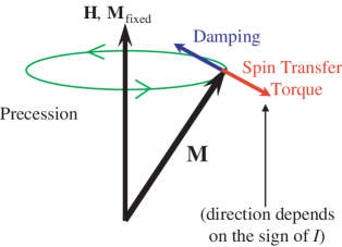
Figure 7: Directions of damping and spin-torque vectors for a simple model discussed in the text.

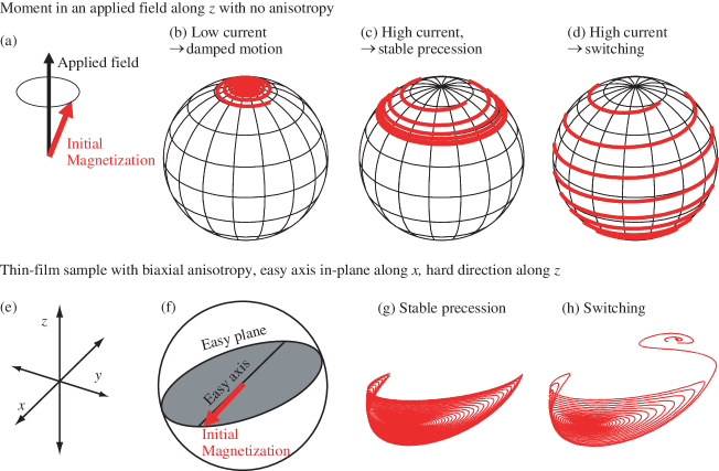
Figure 8: Trajectories of spin-torque-driven dynamics for the magnetization vector ${\bf M}$. (a) Initial magnetic configuration assumed for panels (b,c,d), with the free layer magnetization slightly misaligned from $\hat{\bf z}$, for example due to a thermal fluctuation. For these panels, we assume a sample with no magnetic anisotropy, with ${\bf M}_{\rm fixed}$ and the applied magnetic field aligned in the $\hat{\bf z}$ direction. (b) For currents below a critical current, ${\bf M}$ spirals back toward the low-energy $\hat{\bf z}$ direction on account of magnetic damping. (c) For currents larger than the critical value, the spin transfer torque causes the effective damping to become negative, meaning that ${\bf M}$ spirals away from $\hat{\bf z}$, with a steadily-increasing precession angle. The ultimate result can be either stable steady-state precession at large precession angle (shown in (c)) or magnetic reversal (shown in (d)), depending on angular dependence of the spin torque and damping. (e,f) Geometry assumed for a thin-film magnetic sample with a strong easy-plane anisotropy and a weaker uniaxial anisotropy with stable static magnetic states along the $\pm\hat{\bf x}$ directions. For this geometry, the spin transfer torque from a direct current can also produce either (g) steady-state precession or (h) magnetic reversal from $+\hat{\bf x}$ to $-\hat{\bf x}$.

When a current is applied, the direction of the spin transfer torque predicted by Eq. (25) is either parallel to the damping torque or antiparallel to it, depending on the sign of the current (see Fig. 7). (For the more realistic case of elliptical precession in the presence of magnetic anisotropies, the instantaneous orientations of the spin torque and the damping are not always collinear, but on average over each cycle the spin torque can still be understood as either reinforcing or acting opposite to the damping.) For the sign of the current that produces a spin-torque contribution ${\dot{\bf M}}_{\rm st}$ in the same direction as the damping, there are no current-induced instabilities in the free-layer orientation. The current increases the value of the effective damping, and ${\bf M}$ simply spirals more rapidly back to the ${\bf\hat{z}}$ direction after any perturbation. For small currents of the opposite sign, such that ${\dot{\bf M}}_{\rm st}$ is opposite to the damping but weaker in magnitude, the spin torque just decreases the effective damping, and again nothing exciting happens, at least at zero temperature. (Effects of thermal fluctuations are discussed below.)

When ${\dot{\bf M}}_{\rm st}$ is opposite to the damping torque and of greater magnitude, then following any small perturbation ${\bf M}$ will spiral away from the low-energy configuration along ${\bf\hat{z}}$ to increasing angles – the current destabilizes the orientation with ${\bf M}$ parallel to ${\bf M}_{\rm fixed}$ and may excite large-angle dynamics. In effect, a sufficiently large current drives the damping to be negative, which leads to the amplification of any deviations of ${\bf M}$ from equilibrium. Past this point of instability, the large-angle dynamics excited by spin transfer can fall in two broad classes within the macrospin approximation, depending on the angular dependencies of the spin transfer torque, the damping torque, and the magnetic anisotropy. One possibility, which may occur if the damping torque increases with precession angle faster than the spin torque, is that the initial increase in precession angle may eventually be limited, so that ${\bf M}$ may achieve a state of dynamical equilibrium, precessing continuously at some fixed average angle in response to the direct current (see Fig. 8(c)). In this state, the energy gained from the spin torque during each cycle of precession is balanced by the energy lost to damping. The second possible class of spin-torque-driven magnetic dynamics is that the precession angle may be excited to ever-increasing values until eventually it reaches 180^∘, meaning that ${\bf M}$ is reversed (see Fig. 8(d)).

In real samples, the magnetic anisotropy can generally not be ignored, as we have done so far in the discussion above. The typical sample formed as part of a thin-film magnetic multilayer will have biaxial magnetic anisotropy, consisting of a strong in-plane anisotropy and a weaker uniaxial anisotropy along one of the in-plane axes. In Fig. 8(e)-(g) we consider some of the magnetic trajectories that can be excited by spin transfer for this type of sample, where the easy magnetic axes are assumed to lie along the $\pm\hat{\bf x}$ directions, and ${\bf M}_{\rm fixed}$ and the applied magnetic field are also assumed to point along $\hat{\bf x}$ instead of the $\hat{\bf z}$ direction as in Fig. 8(a)-(d). Within the macrospin approximation, the dynamics of ${\bf M}$ excited by the spin transfer torque can still be calculated by integrating the Landau-Lifshitz-Gilbert equation (Eq. (2)) with the spin-transfer-torque term Eq. (25) included.

Different behavior occurs in different regimes. Consider first in-plane magnetic fields less than the coercive field needed to produce magnetic-field-induced switching. At low temperature, as the current increases, there is generally first a critical current which leads to states of dynamical equilibrium in which ${\bf M}$ undergoes steady-state precession along an approximately elliptical trajectory (see Fig. 8(g)) [30, 141, 142]. For slightly larger currents, the precessing state becomes unstable, and the precession angle for ${\bf M}$ increases until it reaches 180^∘, thereby achieving switching to the state with ${\bf M}$ antiparallel to ${\bf M}_{\rm fixed}$ (Fig. 8(h)). For applied magnetic fields larger than the coercive field, usually only steady-state precessional dynamics are observed (Fig. 8(g)). Additional static and dynamic magnetic states may occur at even larger values of current (see below). If one starts with the free-layer moment ${\bf M}$ oriented antiparallel to the fixed layer, rather than parallel (i.e., with ${\bf M}$ in the $-\hat{\bf x}$ direction rather than $+\hat{\bf x}$), a reversed sign of current is required to produce a negative effective damping, and this can excite steady-state dynamics or switch ${\bf M}$ back to the parallel orientation.

For thin-film samples with the magnetizations of both the fixed and free layers oriented in plane and with their easy axes aligned with the applied magnetic field, it is possible to estimate the threshold current for small-angle excitations in a macrospin picture. The estimation proceeds by integrating over the elliptic orbit for a small precession angle to determine both the energy lost due to damping and the energy gained from the spin torque during each cycle, and determining at what value of current the spin torque overcomes the damping. This leads, for example, to the critical current expression for excitations from an initially parallel magnetic orientation ($\theta=0$)

$$I_{c}={2e\over\hbar}{\alpha\over\eta(0)}\mathcal{V}\mu_{0}M_{s}\left(H+H_{k}+{M_{s}\over 2}\right),$$ (26)

referred to by the article of Katine and Fullerton. Here $\alpha$ is the Gilbert damping, $H$ is the applied magnetic field and $H_{k}$ the strength of the within-plane magnetic anisotropy [28, 143]. The saturation magnetization $M_{\rm s}$ appears in the last factor because of the large thin-film demagnetization effect which favors an in-plane orientation for ${\bf M}$; $M_{\rm s}/2$ is typically much larger than $H$ or $H_{k}$. It is important to note that this threshold describes only the first instability of the free layer to small angle precession. There is a separate threshold for magnetic switching at slightly larger currents, which has a different dependence on magnetic field. Approximate analytical expressions been derived to describe the switching threshold and other boundaries between the different dynamical states that can be driven by spin torques [144, 63, 145]. These phase boundaries are illustrated in Fig. 9 for the case of a magnetic field applied in-plane along the easy axis of the magnetic free layer.

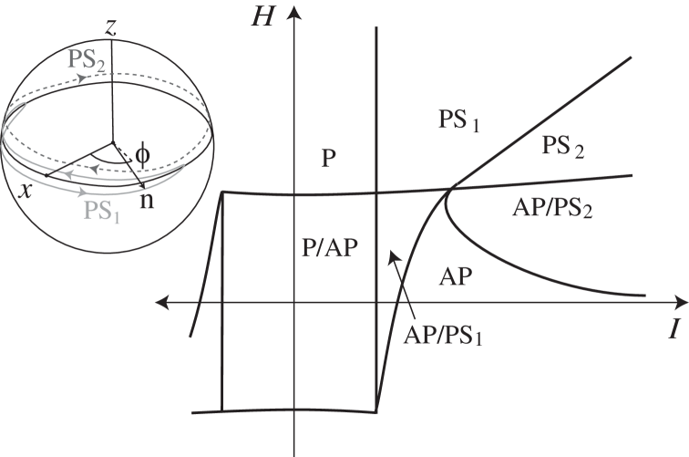
Figure 9: Schematic phase diagram for spin-torque-driven magnetic dynamics of a thin-film free layer in a nanopillar device at zero temperature as a function of current $I$ and a magnetic field $H$ applied in-plane along with magnetic easy axis. P is the static state with the free-layer magnetization parallel to the fixed-layer magnetization, AP is the static antiparallel state, and PS₁ and PS₂ correspond to the steady-state precession states depicted in the inset. Where two states A and B are indicated using the notation A/B, both states are stable at zero temperature. Diagram courtesy of Yaroslaw Bazaliy [145].

One common result of all semiclassical calculations of transport and spin transfer torque for metallic multilayers [62, 63, 122] is that they predict a fairly substantial asymmetry between the differential torque near parallel and antiparallel alignment. That is,

$$\left|{d{\dot{\bf M}}_{\rm st}(\theta)\over d\theta}_{\theta=\pi}\right|>\left|{d{\dot{\bf M}}_{\rm st}(\theta)\over d\theta}_{\theta=0}\right|.$$ (27)

In other words, $B$ is comparable to $A$ in $\eta(\theta)={q/(A+B\cos\theta)}$. This asymmetry arises from the different amounts of spin accumulation for alignments close to parallel as compared to those close to antiparallel. The results suggest that the critical currents for switching out of the antiparallel state in metallic multilayers should be significantly less than those for switching out of the parallel state. However, typically the asymmetry found in the measured critical currents is much less than expected [146]. The degree of asymmetry seems to depend on the sample structure (e.g., on the amount of taper in nanopillar sidewalls), so the discrepancy could result in part from deviations from a completely uniform magnetization state, which might affect either the mechanism of reversal or the degree of spin accumulation. On the other hand, measurements of noise instabilities for magnetizations close to perpendicular [147] suggest an asymmetry consistent with the theoretical expectations.

If ${\bf M}_{\rm fixed}$ and ${\bf M}$ are misaligned within the sample plane by an applied magnetic field or an exchange bias, the critical currents will depend on the angle $\theta_{0}$ between the equilibrium orientations of ${\bf M}$ and ${\bf M}_{\rm fixed}$. This can be understood in a simple way by Taylor-expanding the instantaneous value of the spin torque in the sample plane: ${\dot{\bf M}}_{\rm st}(\theta)\approx{\dot{\bf M}}_{\rm st}(\theta_{0})+[{d\dot{\bf M}}_{\rm st}(\theta_{0})/d\theta](\theta-\theta_{0})$. For current pulses much larger than the threshold needed to produce excitations, the first term can dominate the fast magnetic dynamics that are produced. However, for currents near the critical current this term will generally just cause the equilibrium angle to shift by a small amount as a function of $I$, because it can be opposed by strong anisotropy forces. Near the excitation threshold, it is actually the second term of the Taylor expansion which governs the stability of the static state, because it determines whether the spin torque has the sign to increase or decrease the magnitude of deviations from the equilibrium angle. Dynamical excitations will occur at zero temperature when $d{\dot{\bf M}}_{\rm st}(\theta_{0})/d\theta$ has the correct sign and becomes sufficiently large to overcome the intrinsic damping, so as to cause the free-layer moment to spiral away from its equilibrium orientation with increasing precession angle, as discussed above. In a macrospin picture $I_{c}\propto 1/[d{\dot{\bf M}}_{\rm st}(\theta_{0})/d\theta]\approx 1/\cos(\theta_{0})$ [143, 148].

An additional subtlety that can complicate understanding spin-torque-driven magnetic dynamics is that the magnetization in ferromagnetic devices is never completely spatially uniform, but even in thin-film devices with very small cross section there is some spatial dependence to the magnetization within the layer. This has the consequence that even in devices with electric current flowing strictly perpendicular to the plane the spin current density will have a non-zero spatial component within the plane. These lateral spin currents can produce additional instabilities that lead to the excitation of spatially non-uniform magnetization dynamics within a magnetic layer [127, 135, 149], and in fact these excitations have been observed in devices containing only a single magnetic layer [121] and standard two-magnetic-layer devices [150, 89]. Magnetic excitations that are non-uniform through the thickness of magnetic layers may also be possible [27, 119]. Initial attempts to incorporate lateral spin transport self-consistently with spatially dependent magnetic dynamics in micromagnetic calculations of multilayer devices are under way.

Measurements of Magnetic Dynamics. The main experimental probe of the spin-torque-driven magnetization dynamics is measuring the resistance. The resistance reflects the magnetic configuration through the GMR effect. One signature that a current-driven change in magnetic configuration is due to the spin transfer effect is that it is asymmetric in the direction of the current, for the reasons explained above. In the first identification of a spin transfer effect [25], Tsoi et al. measured a peak in the differential resistance for one direction of the current and not the other. In switching devices [27, 28], for large currents flowing from the fixed layer to the free layer (electrons flowing from free to fixed), the free layer magnetization is driven to be antiparallel to the fixed layer, resulting in the high resistance state, while the opposite current drives the sample to the parallel, low-resistance state. The sign of the torque observed experimentally agrees with the sign predicted by theory.

A sample excited into a state of dc-driven magnetic precession naturally emits a substantial microwave-frequency signal at its electrical contacts. The resistance is changing at microwave frequencies and a dc current is applied, so by Ohm’s law a microwave voltage is generated. This can be detected either in the frequency regime [30, 31] or directly in time-domain measurements [32, 151]. This mode of steady-state precession is of interest for applications which might benefit from a nanoscale oscillator or microwave source that can have a narrow linewidth and is tunable in frequency, see Fig. 10.

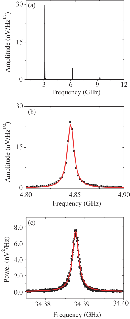
Figure 10: Spectra of voltage oscillations produced by spin-torque-driven steady-state magnetic precession, showing several harmonics and the linewidths of the signals. (a,b) Spectra for all-metal nanopillar samples taken at a temperature of 40 K, courtesy of Ilya Krivorotov. (c) Linewidth for an all-metal point contact sample at room temperature from the NIST, Boulder group [152].

The phase diagram of the spin-transfer-driven dynamics as a function of current, magnetic field, and the direction of magnetic field contains several distinct types of precessional modes and static magnetic states [30, 153]. When one crosses from one mode to another by varying current or field, the frequency of precession can jump, the microwave power output can increase or decrease dramatically, the linewidth can change, and the resistance measured by standard low-frequency techniques generally changes by a small amount, too. When a device is biased near the boundary between two different modes, it often exhibits time-dependent switching behavior between them [154, 141, 151]. The dynamical phase diagram has been mapped in some detail for both in-plane and perpendicular magnetic fields in nanopillar devices [30, 144, 150, 155, 156, 157, 158, 159, 160], and it shows surprisingly good agreement even with the simplest macrospin models, with some exceptions at large currents and for devices in which the magnetic configuration begins in a vortex state [161]. In addition to studies in which the equilibrium orientation of the moments is in the plane, devices have recently been produced in which the magnetic anisotropy of one or more of the magnetic layers is manipulated so that the magnetization points out of plane [68, 69]. Such devices may enable ways to decrease the critical current for switching in memory devices, to increase the switching speed [162], or to produce improved nano-oscillators. Frequency- and time-domain measurements of the different modes of spin-transfer-driven dynamics provide very fertile ground for comparisons with sophisticated micromagnetic simulations of the dynamics, as reported by Berkov and Miltat in their article.

An alternate measurement approach that has recently been exploited is to apply a high frequency input current to drive resonant magnetic precession and look at the static output voltage generated by mixing, a technique referred to as spin-transfer ferromagnetic resonance (ST-FMR) [88, 89, 97, 98, 163, 164]. These measurements, as applied to magnetic tunnel junctions, are discussed in the article by Sun and Ralph.

Effects of Non-Zero Temperature. Spin-torque devices have sufficiently small sizes that temperature-induced fluctuations can have important effects on the magnetic dynamics. At room temperature, the reduced effective damping that can be produced by spin transfer torque can enhance the amplitude of thermal fluctuations even for currents well below the $T=0$ critical current. These enhanced thermal magnetic oscillations can be measured accurately in tunnel junctions [165, 166]. In both tunnel junctions and metallic devices, room temperature thermal fluctuations can also cause magnetic switching to occur at currents that are well below the intrinsic zero-temperature threshold current for spin-transfer-driven instabilities (Eq. (26)). In order to determine the intrinsic critical current for switching, it is necessary to make direct measurements of switching on the typical time scale of ferromagnetic precession near 1 ns, or measure the switching current as a function of temperature and extrapolate to zero temperature, or measure the statistics of switching using current pulses of various lengths and extrapolate to the ns scale.

The linewidths of the microwave signals generated by spin-torque-driven magnetic precession appear to be governed largely by thermal fluctuations that produce deviations from perfectly periodic motion [167, 168]. Point contact devices, in which magnetic precession is excited in a local area of an extended magnetic film can produce narrower linewidths than typical nanopillar devices [169], perhaps because the micromagnetic exchange coupling to the extended film makes them less susceptible to thermal fluctuations. If the effects of thermal fluctuations can be reduced or eliminated, it is likely that the ultimate limit on the linewidths of spin-torque nano-oscillators will be chaotic dynamics of the magnetization [170, 171, 172].

In terms of theory, the role of temperature is an area that is still under development. Transport calculations and determinations of the torque are typically done assuming zero temperature. This approximation is expected to be reasonable because not much about the transport is expected to change with temperature except for scattering rates. There have been a number of theoretical studies of the temperature dependence based on the macrospin approximation [173, 174, 175, 176, 160]. However, as the temperature increases, the macrospin approximation becomes worse. It is possible to include thermal effects into full micromagnetic simulations, but the calculations become quite time consuming and it is very difficult to capture meaningful statistics.

On the Perpendicular Component of the Spin Torque Vector. In discussing the result of Eq. (15), i.e. that one expects essentially all of the transverse spin angular momentum incident onto a normal-metal/ferromagnet interface to be absorbed in producing the spin torque, we made the point that this was only approximately correct; it is not exact. The most important caveat is that classical averaging over the Fermi surface need not necessarily eliminate all transport of transverse spin density away from the interface, particularly for the reflected part of the scattering wavefunction (or for very thin magnetic layers in transmission). One consequence is that the amplitude of the “in-plane” component of the torque can differ somewhat from Eq. (15). In addition, there is the possibility of an additional contribution due to the spin torque in the form

$${\dot{\bf M}}_{\perp}=\eta_{\perp}(\theta){\mu_{\rm B}I\over e\mathcal{V}}~{}\hat{\bf M}\times\hat{\bf M}_{\rm fixed},$$ (28)

oriented perpendicular to the plane defined by ${\bf M}$ and ${\bf M}_{\rm fixed}$, rather than within this plane as in Eq. (25). Note that here the symbol $\perp$ refers to the direction perpendicular to the plane of the magnetizations as opposed to the usage in Eq. (15) where it refers to both components of the spin current transverse to the free layer magnetization. In Fig. 7, this new component of torque would point in or out of the page. The out-of-plane torque component is sometimes referred to as an “effective field” contribution because its form is similar to the torque that would result from a field aligned with the fixed layer magnetization. It can be viewed as a consequence of a small amount of average precession into the ${\bf\hat{y}}$ direction for reflected electrons in our toy models from Section 3.

Calculations incorporating transmission and reflection coefficients computed by ab initio techniques find that the perpendicular component of the torque is small for the materials generally used in metallic multilayer devices. For electrons of a given energy, the out-of-plane component of spin transfer is predicted to be less than 10 %, and typically 1 % to 3 % of the in-plane component [95, 93, 96]. The final magnitude of the bias-dependent part of the out-of-plane torque is expected to be smaller still, due to a cancellation that arises when computing the bias dependence. This cancellation is maximal in the case of a symmetric N/F/N/F/N junction, where it can be understood from a simple symmetry argument.

Consider a junction whose layer structure is perfectly symmetric about a plane at the midpoint of the device, see Fig. 11. Assume that the magnetic moments of the two ferromagnetic layers are oriented in the plane of the sample layers, with an arbitrary angle $\theta$ between them. When a bias is applied to the junction, the resulting spin current density in each lead (each of the outer N layers) will be aligned with the magnetization of the neighboring ferromagnetic layer provided that the electrons that transmit into the lead from the rest of the devices are completely classically dephased. In this case, the spin currents in the outer N layers are oriented in the plane of the two magnetizations, and an out-of-plane spin component of the spin current density can exist only in the middle N layer. If there are no sources or sinks of angular momentum except for the spin torques applied to the magnetic layers (e.g., we assume that there is no angular momentum lost to the excitation of short-wavelength spin wave modes), then angular momentum conservation allows the perpendicular component of spin torques on the ferromagnetic layers to be determined solely from the out-of-plane spin current traveling between the magnetic layers. As a consequence, the out-of-plane spin torques on the two magnetic layers must be equal and opposite. (To be clear, our argument applies only to the perpendicular component of the spin torque and not the in-plane component, because the in-plane spin component of the spin-current density is not zero in the outer N layers, and hence the in-plane spin torques on the ferromagnetic layers are not generally equal and opposite.)

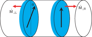
Figure 11: Sample geometry for the perfectly symmetric N/F/N/F/N device assumed in our analysis of the perpendicular component of the spin torque vector. The perpendicular spin torques on the two magnetic layers are equal and opposite.

For an applied bias such that electrons flow from left to right, suppose that the perpendicular spin torque on the right magnetic layer has the value $N_{\perp}$. Now imagine that the bias is reversed, so that electrons flow from right to left. Because of the symmetry of the device, the spin current density in this case can be determined from the first case simply by an appropriate rotation; the answer is that both the direction of the out-of-plane spin component that flows between the two layers and the direction of its flow are reversed, so that (multiplying the two negative signs) the out-of-plane spin current density is actually the same as in the first case. Consequently, the perpendicular spin torque acting on the right magnetic layer due to electrons flowing right to left will again be $N_{\perp}$, the same magnitude and the same sign as for the perpendicular torque on the same (right) magnetic layer due electron flow from left to right. It follows that the perpendicular spin torque on a magnetic layer in a perfectly-symmetric junction is an even function of the bias $V$, as long as conservation of angular momentum can be applied to the spin-transfer process and the classical dephasing processes are complete. Consequently, there is no contribution that is linear in $V$ at zero bias in a symmetric junction, in spite of the fact that ab initio calculations show that electrons at a given energy incident onto a magnetic interface can give non-zero contributions to the perpendicular torque.

In a more microscopic picture, one can see how this result comes about by considering a calculation in which the total perpendicular spin torque is determined by integrating the contributions from all electrons incident onto the symmetric junction from both sides. Following the logic of the symmetry argument above, the perpendicular torque due to incoming electrons in the energy range $d\epsilon$ incident from the left should be the same, $N_{\perp}(\epsilon)d\epsilon$, as for electrons of the same energy incident from the right, as long as we assume that the effect of the applied bias on the scattering potential is sufficiently weak that the electron transmission and reflection amplitudes do not depend explicitly on $V$. For a symmetric junction, any applied voltage bias will offset the electron chemical potential on the two sides of the device by $\pm eV/2$. Therefore, if we consider only elastic scattering processes, the bias-dependent part of the perpendicular torque can be calculated by subtracting the contributions of electrons in the energy range $\epsilon_{F}-eV/2$ to $\epsilon_{F}$ that are no longer incident on the junction from one side, and adding the contribution of the extra electrons in the range $\epsilon_{F}$ to $\epsilon_{F}+eV/2$ that are incident from the other side:

$${\dot{\bf M}}_{\perp}(V)-{\dot{\bf M}}_{\perp}(0)$$ (29)

$$\propto -\int_{\epsilon{{}_{F}}-eV/2}^{\epsilon_{F}}N_{\perp}(\epsilon)d\epsilon+\int_{\epsilon_{F}}^{\epsilon_{F}+eV/2}N_{\perp}(\epsilon)d\epsilon$$

$$\approx {dN_{\perp}(\epsilon_{F})\over d\epsilon}\left({eV\over 2}\right)^{2}.$$

The contributions from the states in the energy ranges $\epsilon_{F}-eV/2$ to $\epsilon_{F}$ and $\epsilon_{F}$ to $\epsilon_{F}+eV/2$ cancel to first order in $eV$, so that the lowest-order contribution to the perpendicular spin torque should go only as $(eV)^{2}$, symmetric in $V$ with no linear term. Even at non-zero biases the perpendicular component of the spin torque is probably very small in most metallic multilayers. Predictions for non-zero values of the perpendicular torque typically arise only under the assumption of coherent transport between ideal interfaces, but in real devices this coherence is generally not present due to interface disorder [91, 96].

For tunnel junctions, the bias-dependent part of the out-of-plane spin torque is predicted to be larger than for metallic multilayers [95, 177]. It remains an open question as to how well our symmetry argument applies to tunnel junctions, because the current may be dominated by a small part of the Fermi surface. In such systems, classical dephasing may not be as complete and therefore in principle a small linear-in-$V$ out-of-plane torque may remain even for a symmetric junction. In addition, for tunnel junctions at high bias, angular momentum loss from hot electrons to the excitation of short-wavelength spin waves might become significant, which would invalidate our arguments because they are based on angular momentum conservation between the conduction electrons and the approximately uniform magnetization mode. Nevertheless, a tight-binding calculation designed to model a symmetric magnetic tunnel junction (in the absence of any short wavelength spin-wave excitations) did predict a bias dependence ${\dot{\bf M}}_{\perp}(V)-{\dot{\bf M}}_{\perp}(0)\propto V^{2}$ [177], consistent with the symmetry argument. For a tunnel junction device with a non-symmetric layer structure none of the symmetry arguments apply, and in this case one should expect that there may be a perpendicular spin torque with a linear dependence on $V$ near zero bias. The potential absence of complete classical dephasing in magnetic tunnel junctions, the consequences of spin-wave excitation by hot electrons, and the effects of non-symmetric layer structures are all interesting questions for future theoretical work, as is the effect of disorder on the out-of-plane torque.

The experimental literature regarding the perpendicular component of spin torque contains some contradictory results. Recent spin-transfer ferromagnetic resonance measurements (ST-FMR) on metallic NiFe/Cu/NiFe devices find no sign of a perpendicular torque at the level of 1 % of the in-plane torque [97], in agreement with the theoretical expectations. However, Zimmler et al. interpreted a measurement on Co/Cu/Co devices [178] of a non-zero slope vs. current for the critical magnetic field for switching $H_{c}(I)$ at 4.2 K as demonstrating a perpendicular torque linear in $V$ with a magnitude about 20 % of the in-plane torque. We are skeptical of this interpretation, and suspect that the observation might be an artifact of heating. The measured slope of $H_{c}(I)$ was not actually constant as a function of $I$ as would be expected from a perpendicular torque, but rather the slope of $H_{c}(I)$ was approximately zero except for combinations of current polarity and magnetic orientation for which the spin torque decreases the effective magnetic damping. This asymmetric rounding of the critical field line can be viewed as a signature of thermally induced fluctuations [173], in that a decreased effective damping can increase the amplitude of thermal fluctuations and therefore decrease the measured switching field at non-zero temperature. Zimmler et al. attempted to correct for this temperature effect in their analysis, but did not consider that the temperature might be varying as a function of current due to heating at 4.2 K.

Spin-transfer FMR measurements on symmetric magnetic tunnel junctions differ from experiments on magnetic multilayers in that the perpendicular torques found in the tunnel junctions are significant [97, 98]. In agreement with our symmetry argument and with more detailed calculations [177], these experiments find that to good accuracy ${\dot{\bf M}}_{\perp}(V)-{\dot{\bf M}}_{\perp}(0)\propto V^{2}$ at low bias for symmetric tunnel junctions, with no contribution to the perpendicular torque that is linear in $V$. An earlier report by Tulapurkar et al. [88] of a perpendicular torque linear in bias near $V=0$ is now believed to be incorrect; the same group has said more recently that this observation may have been an artifact due to a spatially non-uniform magnetic state [98]. The article by Sun and Ralph describes in more detail the similarities and differences between spin torques in metal multilayers and tunnel junctions.

Comparison Between Theory and Experiments. While there is a general consensus about the correct approach for calculating spin transfer torques in magnetic multilayers, there is as of yet no fully quantitative comparison between theory and experiment in metallic multilayers. The primary difficulty is that the torques themselves are generally not measured directly, but only the resulting dynamics as inferred from the time dependent resistance. Spin-transfer-driven ferromagnetic resonance may eventually enable more direct quantitative measurements, but so far this has not been achieved for the in-plane component of the spin-torque in metal multilayers. As described in the article by Berkov and Miltat, attempting to infer the dynamics of a magnetic sample from its time dependent resistance is highly non-trivial and may hide the details of the torque. The problem is particularly complicated because it is difficult to determine simply from resistance measurements the degree to which spin-torque induced excitations are spatially non-uniform.

The most sophisticated calculations can make very good qualitative predictions concerning, for example, the different types of dynamical modes (static or precessional) that are observed experimentally. However, they currently do not match experiment well in more quantitative comparisons, for instance in comparing to the current-dependent amplitude of the microwave signals emitted in the steady-state precession regime (see the article by Berkov and Miltat). Another complication is that there is still some variation experimentally between the behaviors of nominally identical samples. This degree of variability has improved since spin transfer effects were first measured, so that quantities like switching currents and precession frequencies now show good reproducibility. However, other quantities, e.g. microwave linewidths and the positions of transitions between different precession modes, are much more variable. The variability that still exists highlights the importance of achieving improved control over materials and lithography.

5 Domain Walls in Nanowires

In this section we provide a very brief introduction to current-induced domain wall motion. This section is brief compared to the previous section because the articles by Beach, Tsoi, and Erskine, by Tserkovnyak, Brataas, and Bauer, and by Ohno and Dietl together provide a rather comprehensive introduction, review, and summary of open questions for this topic.

Experimentally, current-induced domain wall motion is typically studied in lithographically defined, narrow magnetic wires. The wires are frequently curved or the ends are designed to make it possible to controllably introduce a domain wall into the wire using an applied field. In early experiments, the positions of the domain walls were imaged using techniques such as Magnetic Force Microscopy (MFM) [4, 8] or Scanning Electron Microscopy with Polarization Analysis (SEMPA) [7]. Measuring the positions before and after a current pulses allows estimates of the wall velocities. Alternatively, the locations of the wall could be determined in real time using the Magneto-Optic Kerr Effect (MOKE) [179] or electrically using GMR sandwich structures [5, 6] or through the extra resistance due to anisotropic magnetoresistance (AMR) in a domain wall [180]. Using these various techniques, experimentalists can determine the wall velocity as a function of current and applied magnetic field and compare with theoretical predictions. The level of the comparison is discussed in detail in the article by Beach, Tsoi, and Erskine.

To a first approximation, understanding current-induced domain wall motion is quite simple [1]. Assuming that the electron spins adiabatically follow the magnetization direction, the divergence of the spin current in Eq. (22) gives a torque (actually a torque density, but for the rest of the article we refer to it simply as a torque) on the magnetization of $-({\bf v}_{0}\cdot\bm{\nabla}){\bf M}({\bf r})$. Here, ${\bf v}_{0}$ is a vector in the current direction with magnitude $v_{0}={P|j|\mu_{B}/eM}$, where $P$ is the polarization of the current. If the current is uniform, this torque density simply translates the domain wall in the direction of electron flow with a speed $v_{0}$. There are several factors that complicate this simple description. These factors are described in the three articles by Beach, Tsoi, and Erskine, by Tserkovnyak, Brataas, and Bauer, and by Ohno and Dietl.

The degree to which the spins adiabatically follow the magnetization has been computed in several models [181, 182, 183]. The deviations are small except for rather narrow domain walls. When they are non-negligible, there is an additional torque in the ${\bf M}\times({\bf v}_{0}\cdot\bm{\nabla}){\bf M}$ direction. This torque is referred to as a non-adiabatic torque because it derives from the inability of the electron spins to adiabatically follow the magnetization direction.

Much of the debate on the theoretical description of current-induced domain wall motion is associated with how to describe the damping and whether there is an additional torque in the direction of the non-adiabatic torque [181, 184] that arises from the same processes that lead to damping. This torque, while not related to a true non-adiabatic torque is still sometimes called a non-adiabatic torque. Alternatively, sometimes it is called the beta term, because $\beta$ is the dimensionless parameter that is frequently used to characterize its strength. This contribution is extensively discussed by Tserkovnyak, Brataas, and Bauer. One technical aspect, whether the adiabatic spin transfer torque can be derived from an energy functional, is addressed in the article by Haney, Duine, Núñez, and MacDonald. One of the present authors believes that their argument is incorrect, but disagreement is one of the things that makes an issue an open question.

Just as the dynamics of the free magnetic layers in nanopillars are complicated by the possibility of spatially non-uniform magnetization patterns, so are the dynamics of domain wall motion complicated by non-trivial wall structures. When the domain patterns distort, the motion is no longer simple. Domain walls distort in response to non-adiabatic torques, damping, and the presence of non-uniformities in the sample. The non-uniformities are frequently described as pinning centers. They have been studied extensively in the context of field driven domain wall motion as discussed by both Beach, Tsoi, and Erskine and Ohno and Dietl. Much experimental effort is spent on trying to minimize and understand the effects of these pinning centers.

6 Outlook

In this article, we have tried to highlight some of the open questions in the study of spin transfer torques and provide background material for the succeeding articles. As Katine and Fullerton describe, spin transfer torques should start having commercial impact in the very near future, but there are still important scientific issues to work through. It seems likely that tunnel junctions will be an important system for applications of spin transfer torques. Sun and Ralph discuss what is known about spin transfer torques in magnetic tunnel junctions as well as what we still need to learn.

The dynamics that result from spin transfer torques is the topic of the articles by Berkov and Miltat and by Silva and Rippard. The former focuses primarily on the nanopillar geometry with a free layer that is patterned to have a finite extent. The latter focuses on the fabricated nanocontact geometry in which the free layer is part of an extended thin film. Both show that the agreement between theory and experiment is still incomplete.

The developments in current-induced domain wall motion are more recent than those in magnetic multilayers and tunnel junctions, so applications are still more uncertain. As Beach, Tsoi, and Erskine describe, the experiments are rapidly becoming more sophisticated and more meaningful results are appearing. Tserkovnyak, Brataas, and Bauer describe the rapid progress in the theory of spin transfer torques in these systems. It is likely that experimental progress will challenge these theories and more work will be required.

Most research on spin transfer torques has focused on transition metal ferromagnets, but there are other potentially interesting materials systems. Ferromagnetic semiconductors are potentially exciting because they have magnetizations much smaller than transition metal magnets, so that their moments might be manipulated using spin transfer from much smaller currents than transition metal magnets. While the feasibility of a room-temperature dilute ferromagnetic semiconductor remains to be established, there are fascinating scientific questions to be understood about these materials and their interactions with current. Ohno and Dietl describe the measurements of current-induced domain wall motion in a dilute magnetic semiconductor and a theory that can be used to characterize the electrical and magnetic properties of these systems. Haney, Duine, Núñez, and MacDonald describe a different way of computing spin transfer torques and apply it to novel systems. In particular, they raise the possibility of large spin transfer torques in antiferromagnets.

7 Acknowledgements

We thank Piet Brouwer, Bob Buhrman, Paul Haney and Christian Heiliger for valuable conversations about this manuscript, and many other colleagues (too many to list) who have helped to educate us about spin transfer torques. We also thank Julie Borchers, Arne Brataas, Yongtao Cui, Zhipan Li, Jabez McClelland, Jacques Miltat, Josh Parks, Vlad Pribiag, Kiran Thadani, Hsin-Wei Tseng, and Yaroslav Tserkovnyak for reading the manuscript and offering suggestions for improvement, and Sufei Shi for help with figures. The spin-torque work of DCR is supported by the Office of Naval Research, the NSF (DMR-0605742 and EEC-0646547), and DARPA.

8 Notes on Corrections

This version of the tutorial is modified from the originally-published version. (i) We have corrected algebraic errors in Eq. (13) and modified the discussion in the following paragraphs to correct a mistaken claim that the spin current density in the toy model can be discontinuous at the interface. We thank Claire Baraduc for pointing out the error. (ii) We have corrected an error in the units for the y axes in Figures 10a and 10b.

References

- [1] L. Berger, J. Appl. Phys. 3, 2156 (1978); ibid. 3, 2137 (1979).
- [2] P. P. Freitas and L. Berger, J. Appl. Phys. 57, 1266 (1985).
- [3] C.-Y. Hung and L. Berger, J. Appl. Phys. 63, 4276 (1988).
- [4] L. Gan, S. H. Chung, K. H. Aschenbach, M. Dreyer, and R. D. Gomez, IEEE Trans. Magn. 36, 3047 (2000).
- [5] T. Ono, Y. Ooka, S. Kasai, H. Miyajima, N. Nakatani, N. Hayashi, K. Shigeto, K. Mibu, and T. Shinjo, Mater. Sci. Eng., B 84, 126 (2001).
- [6] J. Grollier, D. Lacour, V. Cros, A. Hamzic, A. Vaurès, A. Fert, D. Adam, and G. Faini, J. Appl. Phys. 92, 4825 (2002).
- [7] M. Kläui, C. A. F. Vaz, and J. A. C. Bland, W. Wernsdorfer, G. Faini and E. Cambril, L. J. Heyderman, Appl. Phys. Lett. 83, 105 (2003).
- [8] M. Tsoi, R. E. Fontana, and S. S. P. Parkin, Appl. Phys. Lett. 83, 2617 (2003).
- [9] P. Grünberg, R. Schreiber, Y. Pang, M. B. Brodsky, and H. Sowers, Phys. Rev. Lett. 57, 2442 (1986).
- [10] C. F. Majkrzak, J. W. Cable, J. Kwo, M. Hong, D. B. McWhan, Y. Yafet, J. V. Waszcak, and C. Vettier, Phys. Rev. Lett. 56, 2700 (1986).
- [11] M. B. Salamon, S. Sinha, J. J. Rhyne, J. E. Cunningham, R. W. Erwin, J. Borchers, and C. P. Flynn, Phys. Rev. Lett. 56, 259 (1986).
- [12] M. D. Stiles, J. Magn. Magn. Mater. 200, 322 (1999); P. Bruno, J. Phys.: Condens. Matter 11, 9403 (1999); D. E. Bürgler, P. Grünberg, S. O. Demokritov, and M. T. Johnson, in Handbook of Magnetic Materials, Vol. 13, ed. K. H. J. Buschow (2001); M. D. Stiles in Ultrathin Magnetic Structures III, J. A. C. Bland and B. Heinrich (Eds.) (Springer Verlag Berlin 2005) p 99; M. D. Stiles in, Nanomagnetism: Ultrathin Films, Multilayers and Nanostructures, D. L. Mills and J. A. C. Bland (Eds.) (Elsevier Amsterdam 2006), p. 51.
- [13] M. N. Baibich, J. M. Broto, A. Fert, F. Nguyen Van Dau, F. Petroff, P. Etienne, G. Creuzet, A. Friederich, and J. Chazelas, Phys. Rev. Lett. 61, 2472 (1988).
- [14] G. Binasch, P. Grünberg, F. Saurenbach, and W. Zinn, Phys. Rev. B 39, 4828 (1989).
- [15] T. McGuire and R. Potter, IEEE Trans. Magn. 11, 1018 (1975); I. A. Campbell and A. Fert, Transport Properties of Ferromagnets, in Ferromagnetic Materials, Vol. 3, E. P. Wohlfarth (Ed.), North Holland, Amsterdam, 1982.
- [16] W. P. Pratt, S.-F. Lee, J. M. Slaughter, R. Loloee, P. A. Schroeder, and J. Bass, Phys. Rev. Lett. 66, 3060 (1991).
- [17] J. Bass and W. P. Pratt, J. Magn. Magn. Mater. 200, 274 (1999).
- [18] S. S. P. Parkin, N. More, and K. P. Roche, Phys. Rev. Lett. 64, 2304 (1990).
- [19] J. Unguris, R. J. Celotta, and D. T. Pierce, J. Appl. Phys. 75, 6437 (1994).
- [20] P. Bruno and C. Chappert, Phys. Rev. Lett. 67, 1602 (1991).
- [21] J. C. Slonczewski, Phys. Rev. B 39, 6995 (1989).
- [22] J. C. Slonczewski, J. Magn. Magn. Mater. 159, L1 (1996); 195, L261 (1999).
- [23] L. Berger, Phys. Rev. B 54, 9353 (1996); J. Appl. Phys. 90, 4632 (2001).
- [24] J. Slonczewski, United States Patent #5,695,864, December 9, 1997.
- [25] M. Tsoi, A. G. M. Jansen, J. Bass, W. C. Chiang, M. Seck, V. Tsoi, and P. Wyder, Phys. Rev. Lett. 80, 4281 (1998).
- [26] J. Z. Sun, J. Magn. Magn. Mater. 202, 157 (1999).
- [27] E. B. Myers, D. C. Ralph, J. A. Katine, R. N. Louie, R. A. Buhrman, Science 285, 867 (1999).
- [28] J. A. Katine, F. J. Albert, R. A. Buhrman, E. B. Myers, D. C. Ralph, Phys. Rev. Lett. 84, 3149 (2000).
- [29] M. Tsoi, A. G. M. Jansen, J. Bass, W.-C. Chiang, V. Tsoi, and P. Wyder, Nature 406, 46 (2000).
- [30] S. I. Kiselev, J. C. Sankey, I. N. Krivorotov, N. C. Emley, R. J. Schoelkopf, R. A. Buhrman, and D. C. Ralph, Nature 425, 380 (2003).
- [31] W. H. Rippard, M. R. Pufall, S. Kaka, S. E. Russek, T. J. Silva, Phys. Rev. Lett. 92, 027201 (2004).
- [32] I. N. Krivorotov, N. C. Emley, J. C. Sankey, S. I. Kiselev, D. C. Ralph and R. A. Buhrman, Science 307, 228, (2005).
- [33] T. Miyazaki and N. Tezuka, J. Magn. Magn. Mater. 139, L231 (1995).
- [34] J. S. Moodera, L. R. Kinder, T. M. Wong, and R. Meservey, Phys. Rev. Lett. 74, 3273 (1995).
- [35] W. H. Butler, X.-G. Zhang, and T. C. Schulthess, and J. M. MacLaren, Phys. Rev. B 63, 054416 (2001).
- [36] J. Mathon and A. Umerski, Phys. Rev. B 63, 220403(R) (2001).
- [37] S. S. P. Parkin, Christian Kaiser, Alex Panchula, Philip M. Rice, Brian Hughes, Mahesh Samant, and See-Hun Yang, Nature Mater. 3, 862 (2004).
- [38] S. Yuasa, T. Nagahama, A. Fukushima, Y. Suzuki and K. Ando, Nature Mater. 3, 868 (2004).
- [39] Y. Huai, F. Albert, P. Nguyen, M. Pakala, and T. Valet, Appl. Phys. Lett. 84, 3118 (2004).
- [40] G. D. Fuchs, N. C. Emley, I. N. Krivorotov, P. M. Braganca, E. M. Ryan, S. I. Kiselev, J. C. Sankey, D. C. Ralph, R. A. Buhrman, and J. A. Katine, Appl. Phys. Lett. 85, 1205 (2004).
- [41] J Hayakawa, S. Ikeda, Y. M. Lee, R. Sasaki, T. Meguro, F. Matsukura, H. Takahashi, and H. Ohno, Jap. J. Appl. Phys. 44, L1267 (2005).
- [42] P. Grünberg, German Patent DE 3820475 C1, June 16, 1988. P. Grunberg, United States Patent #4,949,039, August 14, 1990.
- [43] S. S. P. Parkin United States Patent #6,834,005, December 21, 2004.
- [44] Ultrathin Magnetic Structures I, J. A. C. Bland and B. Heinrich (Eds.) (Springer Verlag Berlin 1994); Ultrathin Magnetic Structures II, B. Heinrich and J. A. C. Bland (Eds.) (Springer Verlag Berlin 1994); Ultrathin Magnetic Structures III, J. A. C. Bland and B. Heinrich (Eds.) (Springer Verlag Berlin 2004); Ultrathin Magnetic Structures IV, B. Heinrich and J. A. C. Bland (Eds.) (Springer Verlag Berlin 2005).
- [45] Nanomagnetism: Ultrathin Films, Multilayers and Nanostructures, D. L. Mills and J. A. C. Bland (Eds.) (Elsevier Amsterdam 2006).
- [46] Spin Dynamics in Confirnd Magnetic Structures I, B. Hillebrands and K. Ounadjela (Eds,) (Springer Verlag Berlin Heidelberg 2001); Spin Dynamics in Confirnd Magnetic Structures II, B. Hillebrands and K. Ounadjela (Eds,) (Springer Verlag Berlin Heidelberg 2003); Spin Dynamics in Confirnd Magnetic Structures III, B. Hillebrands and A. Thiaville (Eds,) (Springer Verlag Berlin Heidelberg 2006).
- [47] Handbook of Magnetism and Advanced Magnetic Materials, 5 Volume Set, H. Kronmüller and S. S. P. Parkin (Eds.) (Wiley 2007).
- [48] Concepts in Spin Electronics S. Maekawa (Ed.) (Oxford Univ. Press 2006).
- [49] Journal of Magnetism and Magnetic Materials, 200, (1999).
- [50] Fulde, P. Electron correlations in molecules and solids. (Springer-Verlag, New York 1995).
- [51] K. Held, and D. Vollhardt, Eur. Phys. J. B 5, 473 (1998).
- [52] I. Yang, S. Y. Savrasov, and G. Kotliar, Phys. Rev. Lett. 8721, 216405 (2001).
- [53] W. Kohn and L. J. Sham, Phys. Rev. 140, A1133 (1965).
- [54] U. von Barth and L. Hedin, J. Phys. C: Solid State Phys. 5, 1629 (1972).
- [55] O. Gunnarsson and B. I. Lundqvist, Phys. Rev. B 13, 4274 (1976).
- [56] R. O. Jones and O. Gunnarsson, Rev. Mod. Phys. 61, 689 (1989).
- [57] Calculated Electronic Properties of Metals by V. L. Moruzzi, J. F. Janak, A. R. Williams (Pergamon, New York, 1978).
- [58] D. C. Langreth and J. W. Wilkins, Phys. Rev. B 6, 3189 (1972).
- [59] C. Vouille, A. Barthélémy, F. Elokan Mpondo, A. Fert, P. A. Schroeder, S. Y. Hsu, A. Reilly, and R. Loloee, Phys. Rev. B 60, 6710 (1999).
- [60] J. Bass and W. P. Pratt, Jr., J. Magn. Magn. Mater. 200, 274 (1999).
- [61] T. Valet and A. Fert, Phys. Rev. B 48, 7099 (1993).
- [62] A. Brataas, G. E. W. Bauer, and Paul J. Kelly, Physics Reports 427, 157 (2006).
- [63] M. D. Stiles and J. Miltat, Topics In Appl. Phys. 101, 225 (2006).
- [64] W. F. Brown, Jr., Phys. Rev. 130, 1677 (1963).
- [65] J. Fidler and T. Schrefl, J. Phys. D, 33, R135 (2000).
- [66] Introduction to the Theory of Ferromagnetism, A. Aharoni, (Oxford University Press, Oxford, 2001).
- [67] In discussions of ferromagnetism, the word “exchange” is used to mean several things, all fundamentally related but nevertheless distinct. This can be confusing. Exchange can be used to describe the electron interactions that give rise to the formation of a moment. It can be used to describe the interaction between a moment and a spin, as is done in the s-d model. It can also be used to describe the interaction between moments on neighboring sites ( and ) that tends to keep the moments aligned, . When we speak of exchange in the context of micromagnetism, it is this last meaning to which we refer.
- [68] S. Mangin, D. Ravelosona, J. A. Katine, M. J. Carey, B. D. Terris, and E. E. Fullerton, Nature Mater. 5, 210 (2006).
- [69] D. Houssameddine, U. Ebels, B. Delaët, B. Rodmacq, I. Firastrau, F. Ponthenier, M. Brunet, C. Thirion, J.-P. Michel, L. Prejbeanu-Buda, M.-C. Cyrille, O. Redon, and B. Dieny, Nature Mater. 6, 447 (2007).
- [70] R. P. Cowburn, J. Phys. D: Appl. Phys. 33, R1, (2000).
- [71] A. Hubert and R. Schäfer, Magnetic Domains: The Analysis of Magnetic Microstructures, (Springer-Verlag, Berlin 1998).
- [72] P. Bruno, Phys. Rev. Lett. 83, 2425 (1999).
- [73] A vortex core is truly only a singularity when the magnetization is required to stay within the plane. In real vortex cores, the magnetization rotates out of the plane and the magnetization pattern is continuous everywhere.
- [74] R. D. McMichael and M. J. Donahue, IEEE Trans. Magn. 33, 4167 (1997).
- [75] L. Landau and E. Lifshitz, Phys. Z. Sowjet. 8, 153 (1935).
- [76] T. L. Gilbert, Armour Research Foundation Project No. A059, Supplementary Report, May 1, 1956 (unpublished). See also T. L. Gilbert, IEEE Trans. Magn. 40, 3443 (2004).
- [77] B. Heinrich, in Ultrathin Magnetic Structures III, J. A. C. Bland and B. Heinrich (eds.) (Springer, Berlin, 2005) p. 143.
- [78] E. Rossi, O. G. Heinonen, and A. H. MacDonald, Phys. Rev. B 72, 174412 (2005).
- [79] R. D. McMichael, D. J. Twisselmann, and A. Kunz, Phys. Rev. Lett. 90, 227601 (2003).
- [80] V. Kamberský, Czech. J. Phys. B 26, 1366 (1976).
- [81] J. Sinova, T. Jungwirth, X. Liu, Y. Sasaki, J. K. Furdyna, W. A. Atkinson, and A. H. MacDonald, Phys. Rev. B 69, 085209 (2004).
- [82] K. Gilmore, Y. U. Idzerda, and M. D. Stiles Phys. Rev. Lett. 99, 027204 (2007).
- [83] Y. Tserkovnyak, A. Brataas, G. E. W. Bauer, Phys. Rev. Lett. 88, 117601 (2002);Y. Tserkovnyak, A. Brataas, G. E. W. Bauer, Phys. Rev. B 66, 224403 (2002); Y. Tserkovnyak,A. Brataas, G. E. W. Bauer, B. I. Halperin, Rev. Mod. Phys. 77, 1375 (2005).
- [84] S. Mizukami, Y. Ando, and T. Miyazaki, Phys. Rev. B 66, 104413 (2002).
- [85] B. Heinrich, Y. Tserkovnyak, G. Woltersdorf, A. Brataas, R. Urban, and G. E. W. Bauer, Phys. Rev. Lett. 90, 187601 (2003).
- [86] N. L. Schryer and L. R. Walker, J. Appl. Phys. 45, 5406 (1974).
- [87] R. D. McMichael and M. D. Stiles, J. Appl. Phys., 97, 10J901 (2005) and references cited therein.
- [88] A. A. Tulapurkar, Y. Suzuki, A. Fukushima, H. Kubota, H. Maehara, K. Tsunekawa, D. D. Djayaprawira, N. Watanabe and S. Yuasa, Nature 438, 339 (2005).
- [89] J. C. Sankey, P. M. Braganca, A. G. F. Garcia, I. N. Krivorotov, R. A. Buhrman, and D. C. Ralph, Phys. Rev. Lett. 96, 227601 (2006).
- [90] For example, J. J. Sakurai, Modern Quantum Mechanics, (Addison-Wesley Publishing, 1985), ch. 3.2.
- [91] X. Waintal, E. B. Myers, P. W. Brouwer, D. C. Ralph, Phys. Rev. B 62, 12317 (2000).
- [92] A. Brataas, Yu. V. Nazarov, and G. E. W. Bauer, Phys. Rev. Lett. 84, 2481 (2000); A. Brataas, Yu.V. Nazarov, and G. E. W. Bauer, Eur. Phys. J. B 22, 99 (2001).
- [93] M.D. Stiles and A. Zangwill, Phys. Rev. B 66, 014407 (2002).
- [94] M.D. Stiles, J. Appl. Phys. 79, 5805 (1996).
- [95] K. Xia, P. J. Kelly, G. E. W. Bauer, A. Brataas, and I. Turek, Phys. Rev. B 65, 220401 (2002).
- [96] M. Zwierzycki, Y. Tserkovnyak, P. J. Kelly, A. Brataas, and G. E. W. Bauer Phys. Rev. B 71, 064420 (2005).
- [97] J. C. Sankey, Y.-T. Cui,J. Z. Sun, J. C. Slonczewski, R. A. Buhrman, D. C. Ralph, Nat. Phys. 4, 67 (2008).
- [98] H. Kubota, A. Fukushima, K. Yakushiji, T. Nagahama, S. Yuasa, K. Ando, H. Maehara, Y. Nagamine, K. Tsunekawa, D.D. Djayaprawira, N. Watanabe, Y. Suzuki, Nat. Phys. 4, 37 (2008).
- [99] M. Johnson and R. H. Silsbee, Phys. Rev. Lett. 55, 1790 (1985).
- [100] F. J. Jedema, H. B. Heersche, A. T. Filip, J. J. A. Baselmans, and B. J. van Wees, Nature 416, 713 (2002).
- [101] N. Tombros, S. J. van der Molen, and B. J. van Wees, Phys. Rev. B 73, 233403 (2006).
- [102] X. Lou, C. Adelmann, S. A. Crooker, E. S. Garlid, J. Zhang, K. S. Madhukar Reddy, S. D. Flexner, C. J. Palmstrom, and P. A. Crowell, Nature Phys. 3, 197 (2007).
- [103] T. Kimura, Y. Otani, and J. Hamrle, Phys. Rev. Lett. 96, 037201 (2006).
- [104] B.T. Jonker, A.T. Hanbicki, D.T. Pierce, and M.D. Stiles, J. Magn. Magn. Mater. 277), 24 (2004).
- [105] See standard texts in quantum mechanics, for example Lectures on Quantum Mechanics, by G Baym (W. A. Benjamin, 1969).
- [106] A. K. Nguyen, H. J. Skadsem, and A. Brataas, Phys. Rev. Lett. 98, 146602 (2007).
- [107] H.-A. Engel, E. I. Rashab, and B. I. Halperin, in Handbook of Magnetism and Advanced Magnetic Materials, H. Kronmüller and S. S. P. Parkin eds. (John Wiley & Sons Ltd., Chichester, UK, 2007), p. 2858 (arXiv:cond-mat/0603306).
- [108] L. Berger, J. Appl. Phys. 93, 7693 (2003).
- [109] G. D. Fuchs, I. N. Krivorotov, P. M. Braganca, N. C. Emley, A. G. F. Garcia, D. C. Ralph, and R. A. Buhrman, Appl. Phys. Lett. 86, 152509 (2005).
- [110] Y. M. Huai, M. Pakala, Z. T. Diao, and Y. F. Ding, Appl. Phys. Lett. 87, 222510 (2005).
- [111] S. Nakamura, S. Haneda, and H. Morise, Jap. J. Appl. Phys. Part 1 45, 3846 (2006).
- [112] H. Meng, J. Wang, and J. P. Wang, Appl. Phys. Lett. 88, 082504 (2006).
- [113] For a thin-film spin transfer device with a circular cross section, a fixed layer structure, and current flowing perpendicularly to the plane, the threshold for spin-torque-driven excitations is given by a particular current density, so that the critical current scales , where is the device radius. Reorientations produced by the current-induced Oersted field will generally occur at a particular field magnitude , so that the threshold current for field-generated reorientations scales , approximately. Therefore a sufficiently small device radius is needed if one desires that the threshold for spin-torque excitations should occur at a lower current than thresholds for magnetic-field-driven reorientations.
- [114] W. H. Rippard, M. R. Pufall, T. J. Silva, Appl. Phys. Lett. 82, 1260 (2003); M. R. Pufall, W. H. Rippard, T. J. Silva, Appl. Phys. Lett. 83, 323 (2003).
- [115] J. Z. Sun D. J. Monsma, D. W. Abraham, M. J. Rooks, and R. H. Koch, Appl. Phys. Lett. 81, 2202 (2002).
- [116] J.-E. Wegrowe, A. Fabian, Ph. Guittienne, X. Hoffer, D. Kelly, J.-Ph. Ansermet, and E. Olive, Appl. Phys. Lett. 80, 3775 (2002).
- [117] Z. Diao, Z. Li, S. Wang, Y. Ding, A. Panchula, E. Chen, L.-C. Wang, and Y. Huai, J. Phys.: Condens. Matter 19, 165209 (2007).
- [118] Y. Acremann, J. P. Strachan, V. Chembrolu, S. D. Andrews, T. Tyliszczak, J. A. Katine, M. J. Carey, B. M. Clemens, H. C. Siegmann, J. Stohr, Phys. Rev. Lett. 96, 217202 (2006).
- [119] Y. Ji, C. L. Chien, and M. D. Stiles, Phys. Rev. Lett. 90, 106601 (2003).
- [120] T. Y. Chen, Y. Ji, and C. L. Chien M. D. Stiles, Phys. Rev. Lett. 93, 026601 (2004).
- [121] B. Özyilmaz, A. D. Kent, J. Z. Sun, M. J. Rooks, and R. H. Koch, Phys. Rev. Lett. 93, 176604 (2004).
- [122] M. D. Stiles, in Handbook of Magnetism and Advanced Magnetic Materials, Volume 5, H. Kronmúler and S. S. P. Parkin (Eds.) (Wiley 2007).
- [123] J. Zhang, P. M. Levy, S. Zhang, V. Antropov, Phys. Rev. Lett. 93, 256602 (2004); P. M. Levy, J. Zhang, Phys. Rev. B 70, 132406 (2004); J. Zhang, P. M. Levy, Phys. Rev. B 71, 184417 (2005); J. Zhang, P. M. Levy, Phys. Rev. B 71, 184426 (2005).
- [124] S. Urazhdin, Phys. Rev. B 69, 134430 (2004).
- [125] J.-E. Wegrowe, M. C. Ciornei, and H.-J. Drouhin, J. Phys.-Cond. Matt, 19, 165213 (2007).
- [126] Y. Tserkovnyak, A. Brataas, and G. E. W. Bauer, Phys. Rev. B 67, 140404(R) (2003).
- [127] M. L. Polianski and P. W. Brouwer, Phys. Rev. Lett. 92, 026602 (2004).
- [128] G. E. W. Bauer, Y. V. Nazarov, D. Huertas-Hernando, A. Brataas, K. Xia, and P. J. Kelly, Mater. Sci. Eng. B-Solid State Mater. Adv. Technol. 84, 31 (2001).
- [129] D. M. Edwards, F. Federici, J. Mathon, and A. Umerski, Phys. Rev. B 71, 054407 (2005).
- [130] P. M. Haney, D. Waldron, R. A. Duine, A. S. Núñez, H. Guo, and A. H. MacDonald Phys. Rev. B 76, 024404 (2007).
- [131] M.D. Stiles and A. Zangwill, J. Appl. Phys. 91, 6812 (2002).
- [132] A. Shpiro, P. M. Levy, and S. Zhang, Phys. Rev. B 67, 104430 (2003).
- [133] L. Berger, IEEE Trans. Magn. 34, 3837 (1998); J. Appl. Phys. 89, 5521 (2001).
- [134] J. Grollier, V. Cros, A. Hamzic, J. M. George, H. Jaffres, A. Fert, G. Faini, J. Ben Youssef, and H. Legall, Appl. Phys. Lett. 78, 3663 (2001); J. Grollier, V. Cros, H. Jaffres, A. Hamzic, J. M. George, G. Faini, J. Ben Youssef, H. Le Gall, and A. Fert, Phys. Rev. B 67, 174402 (2003); A. Fert, V. Cros, J. M. George, J. Grollier, H. Jaffres, A. Hamzic, A. Vaures, G. Faini, J. Ben Youssef, and H. Le Gall, J. Magn. Magn. Mater. 272-276, 1706 (2004).
- [135] M. D. Stiles, J. Xiao, and A. Zangwill, Phys. Rev. B 69, 054408 (2004).
- [136] K. M. Schep, J. B. A. N. van Hoof, P. J. Kelly, G. E. W. Bauer, and J. E. Inglesfield, J. Magn. Magn. Mater. 177, 1166 (1998); M.D. Stiles, and D.R. Penn, Phys. Rev. B 61 3200 (2000); K. Xia, P. J. Kelly, G. E. W. Bauer, I. Turek, J. Kudrnovsky, v. Drchal, Phys. Rev. B 63, 064407 (2001); G. E. W. Bauer, K. M. Schep, K. Xia, and P. J. Kelly, J. Phys. D, 35, 2410 (2002).
- [137] J. C. Slonczewski, J. Magn. Magn. Mater. 247, 324 (2002).
- [138] J. Manschot, A. Brataas, G.E.W. Bauer, Phys. Rev. B 69, 92407 (2004).
- [139] J. Xiao, A. Zangwill, and M. D. Stiles, Phys. Rev. B 70, 172405 (2004).
- [140] J. Xiao, A. Zangwill, and M. D. Stiles, Eur. Phys. J. B 59, 415 (2007).
- [141] I. N. Krivorotov, N. C. Emley, A. G. F. Garcia, J. C. Sankey, S. I. Kiselev, D. C. Ralph, and R. A. Buhrman Phys. Rev. Lett. 93, 166603 (2004).
- [142] T. Devolder, P. Crozat, C. Chapppert, J. Miltat, A. A. Tulapurkar, Y. Suzuki, T, K. Yagami, Phys. Rev. B, 71, 184401 (2005).
- [143] J. Z. Sun, Phys. Rev. B 62, 570 (2000).
- [144] G. Bertotti, C. Serpico, I. D. Mayergoyz, A. Magni, M. d’Aquino, and R. Bonin, Phys. Rev. Lett. 94, 127206 (2005).
- [145] Y. B. Bazaliy, Phys. Rev. B. 76, 140402(R) (2007).
- [146] For example, see P. M. Braganca, I. N. Krivorotov, O. Ozatay, A. G. F. Garcia, N. C. Emley, J. C. Sankey, D. C. Ralph, and R. A. Buhrman, Appl. Phys. Lett. 87, 112507 (2005).
- [147] N. Smith, J. A. Katine, J. R. Childress, M. J. Carey, IEEE Trans. Magn. 42, 114 (2006).
- [148] F. B. Mancoff, R. W. Dave, N. D. Rizzo, R. C. Eschrich, B. N. Engel, and S. Tehrani, Appl. Phys. Lett. 83, 1596 (2003).
- [149] S. Adam, M. L. Polianski, and P. W. Brouwer , Phys. Rev. B 73, 024425 (2006).
- [150] B. Özyilmaz, A. D. Kent, M. J. Rooks, and J. Z. Sun, Phys. Rev. B 71, 140403(R) (2005).
- [151] I. N. Krivorotov, N. C. Emley, R. A. Buhrman, and D. C. Ralph, Phys. Rev. B 77, 054440 (2008).
- [152] W. H. Rippard, M. R. Pufall, S. Kaka, T. J. Silva, and S. E. Russek, Phys. Rev. B 70, 100406(R) (2004).
- [153] I. N. Krivorotov, D. V. Berkov, N. L. Gorn, N. C. Emley, J. C. Sankey, D. C. Ralph, and R. A. Buhrman , Phys. Rev. B 76, 024418 (2007).
- [154] S. Urazhdin, N. O. Birge, W. P. Pratt, J. Bass, Phys. Rev. Lett. 91, 146803 (2003).
- [155] B. Özyilmaz, A. D. Kent, D. Monsma, J. Z. Sun, M. J. Rooks, R. H. Koch, Phys. Rev. Lett. 91, 067203 (2003).
- [156] Z. Li, S. Zhang, Phys. Rev. B 68, 024404 (2003).
- [157] M. Covington, M. AlHajDarwish, Y. Ding, N. J. Gokemeijer, M. A. Seigler, Phys. Rev. B 69, 184406 (2004); M. Covington, A. Rebei, G. J. Parker, M. A. Seigler, Appl. Phys. Lett. 84, 3103 (2004).
- [158] Y. B. Bazaliy, B. A. Jones, S. C. Zhang, Phys. Rev. B 69, 094421 (2004).
- [159] S. I. Kiselev, J. C. Sankey, I. N. Krivorotov, N. C. Emley, M. Rinkoski, C. Perez, R. A. Buhrman, and D. C. Ralph, Phys. Rev. Lett. 93, 036601 (2004).
- [160] J. Xiao, A. Zangwill, and M. D. Stiles, Phys. Rev. B 72, 014446 (2005).
- [161] V. S. Pribiag, I. N. Krivorotov, G. D. Fuchs, P. M. Braganca, O. Ozatay, J. C. Sankey, D. C. Ralph, and R. A. Buhrman, Nature Phys. 3, 498 (2007).
- [162] A. D. Kent, B. Ozyilmaz, and E. del Barco, Appl. Phys. Lett. 84, 3897 (2004).
- [163] J. N. Kupferschmidt, S. Adam, and P. W. Brouwer, Phys. Rev. B 74, 134416 (2006).
- [164] A. A. Kovalev, G. E. W. Bauer, and A. Brataas, Phys. Rev. B 75, 014430 (2007).
- [165] S. Petit, C. Baraduc, C. Thirion, U. Ebels, Y. Liu, M. Li, P. Wang, and B. Dieny, Phys. Rev. Lett. 98, 077203 (2007).
- [166] A. M. Deac, A. Fukushima, H. Kubota, H. Maehara, Y. Suzuki, S. Yuasa, Y. Nagamine, K. Tsunekawa, D. D. Djayaprawira, and N. Watanabe, arXiv:0803.2013.
- [167] J. C. Sankey, I. N. Krivorotov, S. I. Kiselev, P. M. Braganca, N. C. Emley, R. A. Buhrman, and D. C. Ralph Phys. Rev B 72, 224427 (2005).
- [168] J.-V. Kim, V. Tiberkevich, and A. N. Slavin, Phys. Rev. Lett. 100, 017207 (2008).
- [169] W. H. Rippard, M. R. Pufall, and S. E. Russek, Phys. Rev. B 74, 224409 (2006).
- [170] K.-J. Lee, A. Deac, O. Redon, J.-P. Nozieres, and B. Dieny, Nature Mater. 3, 877 (2004).
- [171] D. Berkov and N. Gorn, Phys. Rev. B 71, 052403 (2005).
- [172] Z. Yang, S. Zhang, and Y. C. Li, Phys. Rev. Lett. 99, 134101 (2007)
- [173] E. B. Myers, F. J. Albert, J. C. Sankey, E. Bonet, R. A. Buhrman, and D. C. Ralph, Phys. Rev. Lett. 89, 196801 (2002).
- [174] Z. Li, S. Zhang, Phys. Rev. B 69, 134416 (2004).
- [175] D. M. Apalkov, P. B. Visscher, Phys. Rev. B 72, 180405 (2005); ibid J. Magn. Magn. Mater. 286, 370 (2005).
- [176] S. E. Russek, S. Kaka, W. H. Rippard, M. R. Pufall, T. J. Silva Phys. Rev. B 71, 104425 (2005).
- [177] I. Theodonis, N., Kioussis, A. Kalitsov, M. Chshiev, and W. H. Butler, Phys. Rev. Lett. 97, 237205 (2006).
- [178] M. A. Zimmler, B. Özyilmaz, W. Chen, A. D. Kent, J. Z. Sun, M. J. Rooks, and R. H. Koch Phys. Rev. B 70, 184438 (2004).
- [179] G. S. Beach, C. Knutson, C. Nistor, M. Tsoi, and J. L. Erskine, Phys. Rev. Lett. 97, 057203 (2006).
- [180] M. Hayashi, L. Thomas, Ya. B. Bazaliy, C. Rettner, R. Moriya, X. Jiang, and S. S. Parkin, Phys. Rev. Lett. 96, 197207 (2006).
- [181] G. Tatara, H. Kohno, Phys. Rev. Lett. 92, 086601 (2004).
- [182] X. Waintal and M. Viret, Europhys. Lett. 65, 427 (2004).
- [183] J. Xiao, A. Zangwill, and M. D. Stiles Phys. Rev. B 73, 054428 (2006).
- [184] S. Zhang and Z. Li Phys. Rev. Lett. 93, 127204 (2004).