Mechanical Response of a Small Swimmer Driven by Conformational Transitions

Abstract

A conformation space kinetic model is constructed to drive the deformation cycle of a three-sphere swimmer to achieve propulsion at low Reynolds number. We analyze the effect of an external load on the performance of this kinetic swimmer, and show that it depends sensitively on where the force is exerted, so that there is no general force–velocity relation. We discuss how the conformational cycle of such swimmers should be designed to increase their performance in resisting forces applied at specific points.

Active transport is a most fascinating aspect of the busy life in the cell howard . In the nano-scale world where thermal agitations are wild, miniature machines called molecular motors convert chemical energy—from hydrolysis of ATP molecules—directly into useful mechanical work, in the form of carrying cargo or sliding actin filaments along one another. While it is difficult to imagine fabricating such sophisticated machines in the lab, one may naturally wonder if it is possible to design simpler machines with similar functionalities leigh-etal . In this flavor, an interesting target is an autonomous small scale swimmer Dreyfus ; phoretic , which could later on be steered by coupling to a guiding network or system.

Swimmers at small scale (low Reynolds number) have to undergo non-reciprocal deformations to break the time-reversal symmetry and achieve propulsion taylor . This imposes significant constraints when one wants to design a swimmer with only a few degrees of freedom and strike a balance between simplicity and functionality purcell1 . Recently, there has been an increased interest in such designs 3SS ; swimmer and an interesting example of such robotic micro-swimmers has been realized experimentally using magnetic colloids attached by DNA-linkers Dreyfus .

Here we combine features of simple low Reynolds number hydrodynamic swimmers and elements characteristic of models for chemical molecular motors. We focus on a recently introduced three-sphere swimmer 3SS with the minimal two degrees of freedom. Instead of assuming a prescribed sequence of deformations, we consider these deformations to occur stochastically, as conformational transitions between elongated and shortened states for each of the two degrees of freedom. This gives us a swimmer with a velocity that depends on the transition rates between these states, which in practice could come about via mechanochemical transitions, i.e. due to chemical reactions that are coupled with such mechanical deformations howard . We check that a net velocity requires that detailed balance in the transition rates is broken. Using this simple kinetic model, we study the effect on the swimming velocity of a resisting external force or load: the load clearly drags the swimmer backwards, but also puts elements in compression or extension, thereby modifying the transition rates between extended and shortened states. As a consequence, we find that the performance of the motor strongly depends on where the force is exerted, in contrast to the usual perception that the performance of a swimmer - or a motor - can be summarized in a unique force–velocity relation. Interestingly, the motor performance can in some special cases be increased upon application of the external load, provided it is applied at the right location. More generally, we discuss efficient strategies for optimizing the performance of this swimmer.

Figure 1: Schematics of the configuration space of the three-sphere swimmer. To maintain a net swimming to the right, the deformation moves need to make more clockwise full cycles than counterclockwise ones.

Figure 2: Force balance on the spheres and the linkers for a swimmer moving to the right, when the external load $F$ (acting to the right) is attached to the (a) head, (b) tail, or (c) middle of the swimmer. In each case, it is identified whether each linker is under compression (C) or tension (T), with the value of the force given (underneath).

We start with the swimmer model introduced in 3SS , namely three spheres connected by two linkers of negligible hydrodynamic effect, that cycle in time between extended and short states. For simplicity, we take here all sphere radii to be equal to $a$. We further assume that the lengths of the two arms are $L_{1}(t)=\ell_{1}+u_{1}(t)$ and $L_{2}(t)=\ell_{2}+u_{2}(t)$ with the $u_{i}$’s being small perturbations about the average lengths. For prescribed arm deformations, writing a force balance on each sphere leads an instantaneous net displacement velocity of the swimmer, that can here be written as a series expansion $v(t)=A_{i}{\dot{u}}_{i}+B_{ij}{\dot{u}}_{i}{u}_{j}+C_{ijk}{\dot{u}}_{i}{u}_{j}{u}_{k}+\cdots,$ where the coefficients $A_{i}$, $B_{ij}$, $C_{ijk}$, etc. are purely geometrical prefactors (i.e. involving only the length scales $a$ and $\ell_{i}$). After many cycles, this process gives a vanishing contribution from the linear terms ${\dot{u}}_{1}$ and ${\dot{u}}_{2}$ and from the symmetric combination ${\dot{u}}_{1}u_{2}+{\dot{u}}_{2}u_{1}=d(u_{1}u_{2})/dt$. Thus to leading order the average swimming velocity is

$$V\equiv\langle v\rangle=\frac{K}{2}\langle{\dot{u}}_{1}u_{2}-{\dot{u}}_{2}u_{1}\rangle=K\left\langle\frac{d{\cal A}}{dt}\right\rangle,$$ (1)

where $d{\cal A}$ is the area element in the $(u_{1},u_{2})$ space, and $K=\frac{a}{3}\left[\frac{1}{\ell_{1}^{2}}+\frac{1}{\ell_{2}^{2}}-\frac{1}{(\ell_{1}+\ell_{2})^{2}}\right]$ ag . In other words, to the leading order the swimming velocity is proportional to the area enclosed by the orbit of the cyclic motion in the configuration space of the deformations.

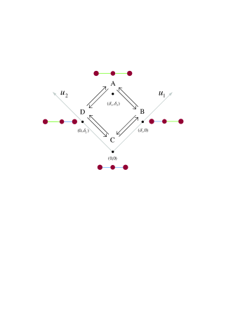
We now focus on a situation where the two arms can be in two states with deformations of either $u_{i}=0$ or $u_{i}=\delta_{i}$, and transit from one to the other in an almost instantaneous fashion. This means that the configuration space of the swimmer will be made of only four distinct states as shown in Fig. 1, which correspond to different values of the pair $(u_{1},u_{2})$, namely: state A for $(\delta_{1},\delta_{2})$, state B for $(\delta_{1},0)$, state C for $(0,0)$, and state D for $(0,\delta_{2})$. We then assign transition rates to the system, corresponding to the average rate of opening and closing of the arms. For example, the transition rate from state A to state B is denoted as $k_{BA}$, and similar notations are used for the 8 rates describing forward and reverse transitions along the cycle

$${\rm A}\xrightleftharpoons[k_{AB}]{k_{BA}}{\rm B}\xrightleftharpoons[k_{BC}]{k_{CB}}{\rm C}\xrightleftharpoons[k_{CD}]{k_{DC}}{\rm D}\xrightleftharpoons[k_{DA}]{k_{AD}}{\rm A}.$$ (2)

For simplicity, and at the cost of motor efficiency, we assume that the transitions occur quite rapidly and seldom, so that they never “overlap.”

We can now calculate the swimming velocity as a function the transition rates. At steady state, the average swimming velocity of the object is given by the probability current $J$ along the A$\rightarrow$B$\rightarrow$C$\rightarrow$D$\rightarrow$A cycle times the net displacement while performing the cycle. This distance $\Delta x$ is simply $K\delta_{1}\delta_{2}$, which yields $V=K\delta_{1}\delta_{2}J.$ The probability current $J$ is a function of the transition rates, which can be obtained from straightforward algebra:

Figure 3: Motor performance function $J(F)/J(0)$ versus the external force, when only one of the rates is enhanced to $1+\epsilon$ while the rest are kept fixed at $1$. The plots correspond to the enhanced rate being (a) $k_{0BA}$, (b) $k_{0CB}$, (c) $k_{0DC}$, and (d) $k_{0AD}$, and $\epsilon=50$. In each case, the dashed (red) line corresponds to the load being attached to the head, the dotted (blue) line corresponds to attachment to the tail, and the solid (green) line is for the middle attachment.

$$J=\frac{k_{AD}k_{DC}k_{CB}k_{BA}-k_{AB}k_{BC}k_{CD}k_{DA}}{\sum_{\rm replace\;A\;by\;B,\;C,\;D}(k_{AD}k_{DC}k_{CB}+k_{AB}k_{BC}k_{CD}+k_{AB}k_{AD}k_{DC}+k_{AD}k_{AB}k_{BC})}.$$ (3)

From the above equation it is clear that if detailed balance holds, then $J$ is zero as the numerator vanishes. Using the average steady state current, we can deduce the average period of one full cyclic motion along A$\rightarrow$B$\rightarrow$C$\rightarrow$D$\rightarrow$A as $T=J^{-1}$. In general a $1\longleftrightarrow 2$ asymmetry in the system, together with breaking the detailed balance at least for one of the transitions, will lead to net motion. For the particular limit where the forward rates are all much higher than the corresponding backward ones ($k_{BA}\gg k_{AB}$, etc.), we find $T=k_{AD}^{-1}+k_{DC}^{-1}+k_{CB}^{-1}+k_{BA}^{-1},$ which simply means that the period for a full cycle is the sum of the time intervals needed to complete each leg of the cycle. As another example, we can assume that all of the equilibrium $k_{\beta\alpha}$’s are equal to $1$ (for the sake of illustration), and that by external action only one of them is modified e.g. $k_{BA}=1+\epsilon$. In this case, it is easy to show that Eq. (3) yields $J=\epsilon/(16+6\epsilon)$, which leads to a velocity proportional to the perturbation if the latter is small and independent of it if the perturbation is very large, as the cycling is then limited by the other three unperturbed transitions. In general, it is easy to see that the slowest leg of the reaction controls the average rate of full cyclic motion.

It is interesting to study the effect of an external load on the velocity of the system and the performance of the motor. When the swimmer is subject to external forces, because of carrying a cargo for example, there are two types of mechanical responses in the system. First, the external forces enter the hydrodynamic force balance on each sphere, and this will introduce a Stokes drag on the sphere as a whole, which is a linearly decaying contribution to the net swimming velocity as a function of force. Second, the transition rates that control the kinetics of the deformations for the two arms of the swimmer are affected by the external forces as they will have to do mechanical work against them to induce the deformations. Depending on where the force is applied, different legs of the kinetic cycle could be affected, and this could lead to a complex mechanical response with the performance of the motor depending on the location of the load. The force-dependent kinetic rates will yield a net current $J(F)$, which combines with the Stokes response to give the swimming velocity as

$$V(F)=-\frac{F}{18\pi\eta a_{R}}+V_{0}\;J(F)/J(0),$$ (4)

where $V_{0}$ is the swimming velocity at zero force, $\eta$ is the viscosity of the solvent, and $a_{R}$ is a renormalized hydrodynamic radius note .

The transition rates are modified in the presence of external forces, because the mechanical energy enters the balance of probability of the different states and transitions among them. If there is a transition from $\alpha\rightarrow\beta$ that corresponds to an extension by a factor of $\delta$, then under a positive tension $f$ the rate of $\alpha\rightarrow\beta$ transitions is increased by a factor of $\exp(fx/k_{\rm B}T)$ while the rate of $\beta\rightarrow\alpha$ transition is decreased by a factor of $\exp(-fx^{\prime}/k_{\rm B}T)$ where typically $x=\theta\delta$ is the distance between state-$\alpha$ and the energy barrier and $x^{\prime}=(1-\theta)\delta$ is the distance between the energy barrier and state-$\beta$ ($\theta$ between $0$ and $1$). Thus the ratio between the two transitions rates (i.e. the $\alpha\rightarrow\beta$ rate divided by the $\beta\rightarrow\alpha$ rate) changes under a tension $f$ by a factor of $\exp(fd/k_{\rm B}T)$ as required by the Boltzmann formula (equilibrium populations between state-$\alpha$ and state-$\beta$ under $f$).

Table 1: The algebraic force $f_{\beta\alpha}$ which should be used in Eq. (5) to calculate the forward rates. The values for the corresponding reverse rates can be obtained via $f_{\beta\alpha}=-f_{\alpha\beta}$.

transition	head	tail	middle
$A\rightarrow B$	$+\frac{1}{3}F$	$-\frac{2}{3}F$	$+\frac{1}{3}F$
$B\rightarrow C$	$+\frac{2}{3}F$	$-\frac{1}{3}F$	$-\frac{1}{3}F$
$C\rightarrow D$	$-\frac{1}{3}F$	$+\frac{2}{3}F$	$-\frac{1}{3}F$
$D\rightarrow A$	$-\frac{2}{3}F$	$+\frac{1}{3}F$	$+\frac{1}{3}F$

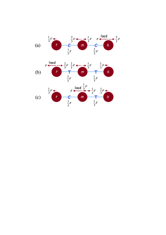
In our system, the value of the force under which each arm should close or open depends on where the load is applied. Figure 2 shows the break down of the mechanical force balance on each sphere, and the corresponding forces endured by each linker, for the three different positions of the load. When the resisting force is attached to the head of the swimmer, both linkers are under compressional forces, and the compression force on the right arm—nearer to the load—is larger than that of the left arm by a factor of two. Attaching the load at the tail creates a similar pattern of tensional forces. If the force acts on the middle sphere, the left arm is under compression and the right arm is under tension.

Using the above definition, the transition rates from a conformation state $\alpha$ to another state $\beta$ can be written as

$$k_{\beta\alpha}=k_{0\beta\alpha}\;\exp\left(\frac{1}{2}\frac{f_{\beta\alpha}\delta_{i}}{k_{\rm B}T}\right),$$ (5)

where $f_{\beta\alpha}$ is the force endured by the linker $i$ that undergoes a deformation during the $\alpha\rightarrow\beta$ transition, and $\theta=1/2$ is assumed for simplicity. The sign of $f_{\beta\alpha}$ is determined by whether the transition (deformation) is helped $(+)$ or opposed $(-)$ by the force acting on the linker. The values of $f_{\beta\alpha}$ are given in Table 1 for the forward reaction rates for the different locations of the load. Note that by definition $f_{\beta\alpha}=-f_{\alpha\beta}$, which can be readily used to calculate the reverse rates.

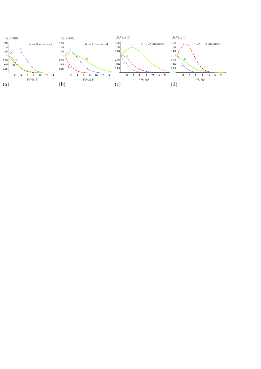
The force-dependent rates [from Eq. (5) and Table 1] can be used in Eq. (3) to calculate the current $J(F)$, which determines the swimming velocity under the effect of an external load $F$. From Eq. (4), it appears that the normalized current $J(F)/J(0)$ is a quantitative measure of how the ability of the motor to generate propulsion is affected by the presence of the load. In Fig. 3, this “motor performance function” is plotted against the external force for the particular example discussed above (in which only one of the forward rates is enhanced to $1+\epsilon$ while the rest of the rates are set to unity), and $\delta_{1}=\delta_{2}\equiv\delta$ is assumed for simplicity. Figure 3a corresponds to when the $A\rightarrow B$ (contraction of the left arm) transition rate is enhanced, and it shows that attaching the load to the head or the middle for both of which the left arm is under a compression of $\frac{1}{3}F$ quickly decreases the performance of motor. On the other hand, attaching the load to the tail of the swimmer, which puts the left arm under a tension of $\frac{2}{3}F$, actually helps the motor initially for forces of up to $3k_{\rm B}T/\delta$ or so, before eventually hampering the performance at large forces. One notes that the force across the left arm actually helps the $A\rightarrow B$ transition when the load is at the head or the middle, and opposes it when it is at the tail. It thus seems that the performance of the motor is best when the rate is enhanced for the deformation which is most hampered by the external load. In other words, the best strategy seems to be to try and make the performances of the different legs of the reaction cycle as uniform as possible, as the total velocity is controlled by the weakest performance in the cycle. The same pattern can be seen in Figs. 3b–3d. Another interesting feature that can be seen is that when the load is at the middle and the condition is right for improved performance (see above) the system seems to endure comparatively much stronger forces: in Figs. 3b and 3c one can see that the performance is significant for loads of up to about $12k_{\rm B}T/\delta$. This is presumably because attaching the load to the middle creates a more balanced distribution of the forces in the linkers (still of opposite nature but of equal magnitudes; see Fig. 2 and Table 1).

Even when the performance of the motor is increased by the opposing force, one still has a decreasing trend for the swimming velocity because of the Stokes drag term in Eq. (4). Using a linear approximation for $J(F)\simeq J_{0}(1+cF\delta/k_{\rm B}T)$ at small forces (where $c$ is a positive constant of order unity), one can write Eq. (4) as $V(F)=V_{0}\left[1-\left(\frac{1}{18\pi\eta a_{R}V_{0}}-\frac{c\delta}{k_{\rm B}T}\right)F\right],$ which implies that for forces much smaller than the thermal activation force $k_{\rm B}T/\delta$ the increased motor performance can lead to increased swimming velocity if the viscous drag on the swimmer is larger than the thermal activation force. While this could be extremely difficult to achieve as it requires unrealistically high swimming velocities, it is an interesting fundamental possibility that increased swimming velocity can be achieved upon exerting opposing forces.

In conclusion, we have proposed and studied a simple model of a low Reynolds number swimmer driven by a kinetic engine. The main result is that the ability of this swimmer to carry a load or to resist an opposing force depends on where the load or the force is applied. This is not linked to the stochastic nature of the present motor, but also holds for a motor driven by a prescribed sequence of internal stresses (to which the applied stresses add up). Altogether, this shows that the description of such machines can go beyond a simple force–velocity relation, more complex and maybe richer in functionality.

References

- (1) J. Howard, Mechanics of Motor Proteins and the Cytoskeleton (Sinauer, New York, 2000).
- (2) E.R. Kay, D.A. Leigh, and F. Zerbetto, Angew. Chem. Int. Ed. 46, 72 (2007).
- (3) R. Dreyfus, J. Baudry, M.L. Roper, M. Fermigier, H.A. Stone, J. Bibette, Nature 437, 862 (2005).
- (4) W.F. Paxton et al., J. Am. Chem. Soc. 126, 13424 (2004); S. Fournier-Bidoz et al., Chem. Comm., 441-443 (2005); N. Mano and A. Heller, J. Am. Chem. Soc. 127, 11574 (2005); R. Golestanian, T.B. Liverpool, and A. Ajdari, Phys. Rev. Lett. 94, 220801 (2005); New J. Phys. 9, 126 (2007); G. Rückner and R. Kapral, Phys. Rev. Lett. 98, 150603 (2007); J.R. Howse et al., Phys. Rev. Lett. 99, 048102 (2007).
- (5) G.I. Taylor, Proc. Roy. Soc. London A 209, 447-461 (1951).
- (6) E.M. Purcell, American Journal of Physics 45, 3-11 (1977).
- (7) A. Najafi and R. Golestanian, Phys. Rev. E 69, 062901 (2004).
- (8) J.E. Avron et al., Phys. Rev. Lett. 93, 186001 (2004); R. Dreyfus et al., Eur. Phys. J. B 47, 161(2005); I.M. Kulic et al. Europhys. Lett. 72, 527 (2005); A. Lee et al., Phys. Rev. Lett. 95, 138101 (2005); A. Najafi and R. Golestanian, J. Phys.: Condens. Matter 17, S1203 (2005); B.U. Felderhof, Phys. Fluids 18, 063101 (2006); E. Gauger and H. Stark, Phys. Rev. E 74, 021907 (2006); A.M. Leshansky, Phys. Rev. E 74, 012901 (2006); D. Tam and A.E. Hosoi, Phys. Rev. Lett. 98 068105 (2007); D.J. Earl et al., J. Chem. Phys. 126 064703 (2007); C.M. Pooley and A.C. Balazs, Phys. Rev. E 76, 016308 (2007); C.M. Pooley et al., arXiv:0705.3612; K. Kruse et al., unpublished.
- (9) R. Golestanian and A. Ajdari, arXiv:0711.3700.
- (10) For the renormalized hydrodynamic radius in Eq. (4), we find which should be expanded in 2nd order of the deformations to keep the same order of terms in the perturbation theory.