A method for exploiting domain information in astrophysical parameter estimation

Abstract

I outline a method for estimating astrophysical parameters (APs) from multidimensional data. It is a supervised method based on matching observed data (e.g. a spectrum) to a grid of pre-labelled templates. However, unlike standard machine learning methods such as ANNs, SVMs or k-nn, this algorithm explicitly uses domain information to better weight each data dimension in the estimation. Specifically, it uses the sensitivity of each measured variable to each AP to perform a local, iterative interpolation of the grid. It avoids both the non-uniqueness problem of global regression as well as the grid resolution limitation of nearest neighbours.

Max Planck Institute for Astronomy, Heidelberg, Germany

1. Introduction

Consider the problem of estimating the astrophysical parameters (APs) of a star from its spectrum using a grid of pre-labelled spectra. Let ${\vec{p}}=\{p_{i}\}$, $i=1\ldots I$ be the data vector (spectrum or multiband photometry) and ${\vec{\phi}}=\{\phi_{j}\}$, $j=1\ldots J$ be the AP vector (e.g. ${\rm T}_{\rm eff}$, $\log g$, etc.). Standard approaches involve performing a global regression on the grid to infer the mapping $\vec{\phi}=g(\vec{p})$, using, for example, a artificial neural network (ANN) (e.g. Bailer-Jones et al. 1998) or a support vector machine (SVM) (e.g. Tsalmantza et al. 2006).

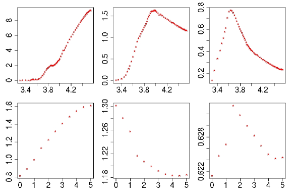
Although these methods meet with reasonable success, they have problems when it comes to estimating multiple APs, in particular if some APs have a relatively weak signature (as is the case with $\log g$ and [Fe/H]: compare the vertical scales in Fig. 1). To overcome this we should weight the variables according to their sensitivity with respect to the APs of interest. In principle, ANNs and SVMs implicitly learn this weighting from the data, but this is difficult with many noisy variables. Furthermore, a global regression approach is strictly flawed, because while the photon counts in a band varies uniquely with the APs, the converse is not true (Fig. 1). The global regression is trying to solve an inverse problem and the lack of uniqueness could lead to a poor fit. This degeneracy problem is exacerbated at low spectral resolution and by noise.

Figure 1.: Variation of photon counts with $\log$ (${\rm T}_{\rm eff}$) (top) and $\log g$ (bottom) in three filters (bands). A $J$-dimensional fit to each band (independently) is a forward model. This is a true function (unlike a fit to the inverse).

2. Basic idea

The new algorithm addresses these issues by explicit use of the sensitivities, $S_{ij}(\vec{\phi})=\frac{\partial p_{i}}{\partial\phi_{j}}$, of each band $i$ to each AP $j$. These are estimated by fitting a (smooth) function, ${\hat{p}_{i}}=f_{i}(\vec{\phi})$ to each band, which I refer to as the forward model (Fig. 1). Sensitivities are estimated from these via first differences. These are used to improve the commonly-employed nearest neighbour (or $\chi^{2}$ minimization) technique. We locally interpolate the grid, defining “optimal” directions for interpolation using the sensitivities, and predicting the photon counts at off-grid points using the forward model.

3. The algorithm

Figure 2.: Sketch of the local iteration principle (described in the text) for $I=1$ and $J=1$.

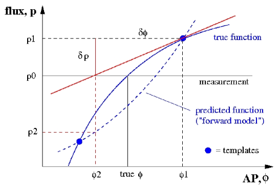
Task: estimate APs of measured vector $\vec{p}_{0}$. The core algorithm (for $I=1,J=1$) is as follows, where subscripts refer here to iterations (see Fig. 2)

1. Fit the forward model to the grid, $\hat{p}=f({\vec{\phi}})$

2. Initialize: find nearest grid neighbour to $\vec{p}_{0}$. Call this $({\vec{p}_{1}},{\vec{\phi}_{1}})$

3. Use the forward model to calculate the local sensitivities, $\frac{\partial\phi}{\partial p}$

4. Calculate the discrepancy (residual), $\delta p_{n}=p_{n}-p_{n-1}$ ($=p_{1}-p_{0}$ for the first iteration)

5. Make a step in AP space, $\phi_{n+1}=\phi_{n}-\left(\frac{\partial\phi}{\partial p}\right)_{\phi_{n}}\delta p_{n}$. This is the new AP prediction

6. Use the forward model to predict the corresponding (off-grid) flux, $p_{n+1}$

7. Iterate steps 3–6

For the general case of $I>1$, step 5 is simply an average over the update calculate for each band, i.e. $\delta\phi=-\sum_{i}\frac{\partial\phi_{j}}{\partial p_{i}}\,\delta p_{i}$. For multiple APs ($J>1$), we can write this in matrix format as $\delta\vec{\phi}=-R\,\delta{\vec{p}}$, where $R=[R_{ji}]$ is the $J\times I$ matrix of reciprocal sensitivities, i.e. $R_{ji}=S_{ij}^{-1}$ (mathematical rigour being sacrificed to some degree). The actual algorithm is a bit more complex (e.g. modified step size).

4. Application and results

I apply the algorithm to a set of synthetic optical photometry of stars showing variation in ${\rm T}_{\rm eff}$ and $\log g$. The $I=11$ photometric bands are part of a system originally designed for Gaia (Jordi et al. 2006). The data show a large variation in APs (Fig. 4), and the grid is quite sparse, comprising just 233 objects. The test set contains 234 objects, with no AP combinations in common between the grid and test set. The signal-to-noise ratio of the test set has been reduced to 10 per band.

The algorithm applied is actually a simpler version of the general case described above: the forward model in steps 3 and 6 is a local linear interpolation (i.e. a plane) of the neighbours in AP space (not data space!) to the current point under consideration. Thus the forward models are robust but suboptimal (as we are no longer taking advantage of the reasonable assumption that $p_{i}=f_{i}(\vec{\phi})$ is smooth).

Figure 3.: AP estimate vs. iteration number for for two sources (left and right), showing examples of correct and incorrect convergence. The horizontal line shows the true parameters.

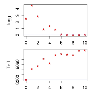
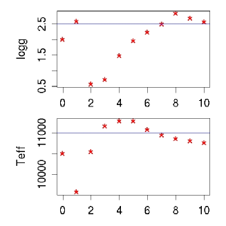
The progress of the algorithm in terms of the AP estimates is demonstrated in Fig. 3 for two of the 234 test cases. These have been selected to demonstrate both good and poor convergence for the two APs.

Figure 4.: Parameter estimation residuals for $\log g$ (left) and $\log$ (${\rm T}_{\rm eff}$) (right).

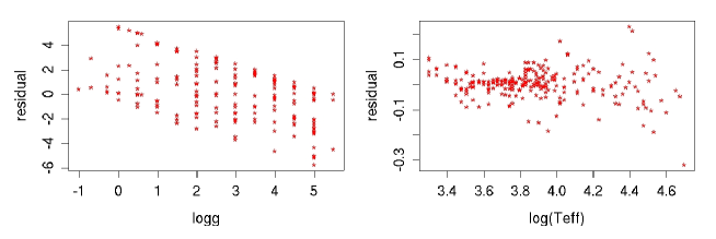
The residuals of the estimates over all 234 objects are shown in Fig. 4, plotted against the true APs. The RMS errors are 1.65 dex in $\log g$ and 0.042 dex in $\log$ (${\rm T}_{\rm eff}$) (corresponding to 480 K at 5000 K). These compare to 0.99 dex for $\log g$ and 0.028 dex for $\log$ (${\rm T}_{\rm eff}$) (320 K at 5000 k) for an SVM model trained and tested on the same data. The systematic error in $\log g$ is also seen with the SVM and is characteristic of the weak AP problem (but not, I believe, unassailable).

5. Conclusions

The algorithm currently performs slightly worse than one of the best generic regression algorithms available (an SVM), yet this is not bad considering that (a) it is in an early stage of development, and (b) the results were obtained using a (suboptimal) linear forward model. Unlike ANNs, the dimensionality of the algorithm’s fitting depends on the number of APs ($J$), not the number of data dimensions ($I$), so it should scale well to typical spectral problems ($J$ is a few, $I$ is a few thousand). Moreover, the method has the ability to detect and report multiple solutions which arise from degeneracies in the data (see Fig. 1).

Acknowledgments.

I thank C. Tiede and K. Smith for useful discussions.

References

Bailer-Jones, C.A.L., Irwin, M., von Hippel, T., 1998, MNRAS, 298, 361

Jordi, C., Hoeg, E., Brown, A.G.A., et al., 2006, MNRAS, 367, 290

Tsalmantza, P., Kontizas, M., Bailer-Jones, C.A.L., et al., 2007, A&A, 470, 761