INSTITUT NATIONAL DE RECHERCHE EN INFORMATIQUE ET EN AUTOMATIQUE

Building the Tangent and Adjoint codes of the Ocean General Circulation Model OPA with the Automatic Differentiation tool TAPENADE
M.H. Tber — L. Hascoët — A. Vidard — B. DauvergneN° 6372
Novembre 2007

Abstract: The ocean general circulation model OPA is developed by the LODYC team at Paris VI university. OPA has recently undergone a major rewriting, migrating to FORTRAN95, and its adjoint code needs to be rebuilt. For earlier versions, the adjoint of OPA was written by hand at a high development cost. We use the Automatic Differentiation tool TAPENADE to build mechanicaly the tangent and adjoint codes of OPA. We validate the differentiated codes by comparison with divided differences, and also with an identical twin experiment. We apply state-of-the-art methods to improve the performance of the adjoint code. In particular we implement the Griewank and Walther’s binomial checkpointing algorithm which gives us an optimal trade-off between time and memory consumption. We apply a specific strategy to differentiate the iterative linear solver that comes from the implicit time stepping scheme.

Key-words: OPA, general circulation model, TAPENADE, Automatic Differentiation, reverse mode, Adjoint Code, Checkpointing

Construction des codes Tangent et Adjoint du modèle de circulation générale océanique OPA par l’outil de Différentiation Automatique TAPENADE

Résumé : Le modèle de circulation générale océanique OPA est développé par l’équipe LODYC de l’université Paris VI. La nouvelle version 9 d’OPA constitue une évolution majeure, avec en particulier une migration vers FORTRAN95. Les codes Linéaire Tangent et Adjoint d’OPA, qui auparavant étaient écrits à la main, doivent donc être redéveloppés. Nous utilisons l’outil de Différentiation Automatique TAPENADE pour construire les codes Tangent et Adjoint d’OPA 9. Nous validons les dérivées obtenues par comparaison avec les Différences Divisées et sur deux applications test incluant des expériences jumelles. Nous utilisons le schéma de checkpointing récursif binomial de Griewank et Walther pour améliorer les performances du code adjoint. Nous utilisons une stratégie spécifique pour différentier le solveur linéaire itératif provenant du schéma implicite d’avancement en temps. Nos résultats montrent un coût raisonnable, tant en consommation mémoire que pour le temps d’exécution de l’adjoint.

Mots-clés : OPA, Circulation Océanique, TAPENADE, Différentiation Automatique, mode inverse, Code Adjoint, Checkpointing

1 Introduction

The development of tangent and adjoint models is an important step in addressing sensitivity analysis and variational data assimilation problems in Oceanography. Sensitivity analysis is the study of how model output varies with changes in model inputs. The sensitivity information given by the adjoint model is used directly to gain an understanding of the physical processes. In data assimilation, one considers a cost function which is a measure of the model-data misfit. The adjoint sensitivities are used to build the gradient for descent algorithms. Similarly the tangent model is used in the context of the incremental algorithms [3] to linearize the cost function around a background control. For the previous version 8 of the Ocean General Circulation Model OPA [17], Weaver et al [22] developed the numerical tangent and adjoint codes by hand using classical techniques [5, 19]. Since then, the OPA model has undergone a major update. Particularly the new versions are fully rewritten in FORTRAN95. In this paper, we report on the development of tangent and adjoint codes of OPA using the Automatic Differentiation (AD) tool TAPENADE [12]. A brief description of the OPA model and the configuration used in this work is given in the next section. In section 3 we present the principles of AD and how they are reflected into the functionalities of the AD tool TAPENADE. In section 4 we focus on the most interesting difficulties that we encountered in the application of AD to such a large code. Section 5 shows some experiments that validate our derivatives and presents two illustrative applications, focusing on computational aspects rather than implications for oceanography. An outlook of further work is given in the conclusion.

2 The Ocean General Circulation Model OPA

Developed by the LODYC team at Paris VI university, OPA is a flexible ocean circulation model that can be used either in a regional or in a global ocean configuration. OPA is the ocean model component of NEMO (Nucleus For European Modelling of the Ocean) and is widely used in the scientific community. Moreover it is becoming a major actor in operational oceanography (Mercator, ECMWF, UK-Met office) Its formulation is based on the so-called primitive equations for the temporal evolution of ocean velocity currents, temperature and salinity in its three horizontal and vertical dimensions. These equations are derived from Navier-Stokes equations coupled with a state equation for water density and heat equation, under Boussinesq and hydrostatic approximations.

Let us introduce the following variables: $\mathbf{U}$ the velocity vector, $\mathbf{U}=\mathbf{U}_{h}+w\mathbf{k}$ (the subscript $h$ denotes the local horizontal vector), $T$ the potential temperature, $S$ the salinity, $p$ the pressure and $\rho$ the in-situ density. The vector invariant form of the primitive equations in an orthogonal set of unit vectors linked to the earth are written as follows

$$\left\{\begin{array}[]{lcl}\dfrac{\partial\mathbf{U}_{h}}{\partial t\vphantom{P_{P}}}&=&-\left[\left(\nabla\times\mathbf{U}\right)\times\mathbf{U}+\dfrac{1}{2}\nabla\left(\mathbf{U}\right){}^{2}\right]_{h}-f\mathbf{k}\times\mathbf{U}_{h}-\dfrac{1}{\rho_{0}}\nabla_{h}p+\mathbf{D}^{\mathbf{U}}\\ \dfrac{\partial p\vphantom{P^{P}}}{\partial z\vphantom{P_{P}}}&=&-\rho g\\ \nabla\cdot\mathbf{U}\vphantom{P^{P}P_{P}}&=&0\\ \dfrac{\partial T\vphantom{P^{P}}}{\partial t\vphantom{P_{P}}}&=&-\nabla\cdot\left(T\mathbf{U}\right)+D^{T}\\ \dfrac{\partial S\vphantom{P^{P}}}{\partial t\vphantom{P_{P}}}&=&-\nabla\cdot\left(S\mathbf{U}\right)+D^{S}\\ \rho\vphantom{P^{P}}&=&\rho\left(T,S,p\right)\end{array}\right.$$

where $\nabla$ is the generalized derivative vector operator, $t$ the time, $z$ the vertical coordinate, $\rho_{0}$ a reference density, $f$ the Coriolis acceleration, and $g$ the gravity acceleration. $\mathbf{D}^{\mathbf{U}},$ $D^{T}$ and $D^{S}$ are the parametrization of small scale physics for momentum, temperature and salinity, including surface forcing terms. A full description of the model basics, discretization, physical and numerical details can be found in [17].

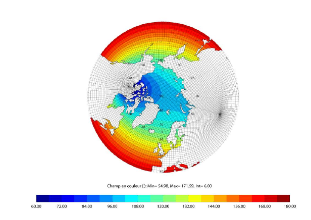
Through this paper, OPA is used in its global free surface configuration ORCA-2. In this configuration the model uses a rotated grid with poles on North America and Asia in order to avoid the singularity problem on the North Pole. The space resolution is roughly equivalent to a geographical mesh of 2° by 1.3° with a meridional resolution of 0.5° near the Equator (see figure 1). The Vertical domain, spreading from the surface to a depth of 5000m, is meshed using 31 levels with levels 1 to 10 in the top 100 meters. The time step is 96 minutes so that there are 15 time steps per day. The model is forced by heat, freshwater, and momentum fluxes from the atmosphere and/or the sea-ice. The solar radiation penetrates the upper layers of the ocean. Zero fluxes of heat and salt are applied through the bottom. On the lateral solid boundaries a no-slip condition is also applied. Initialization of the model for temperature and salinity is based on the Levitus et al. (1998) climatology with a null initial velocity field. For more details about the space time-domain and the ocean physics of ORCA-2, we refer to the page dedicated to this configuration in the official website of NEMO-OPA.

The configuration ORCA-2 is routinely used by MERCATOR/Meteo-France to compute the oceanic component of their seasonal forecasting system. The size of OPA-9, 200 modules defining 800 procedures with over 100 000 lines of FORTRAN95, makes it the largest application differentiated by TAPENADE to date. The computational kernel which is actually differentiated accounts for 330 procedures.

Figure 1: ORCA 2 Mesh

3 Principles of AD and the tool TAPENADE

TAPENADE [12] is an AD tool developed by the Tropics team at INRIA. Given the source of an original program that evaluates a mathematical function, and given a selection of input and output variables to be differentiated, TAPENADE produces a new source program that computes the partial derivatives of the selected outputs with respect to the selected inputs.

Basically, TAPENADE does that by inserting additional statements into a copy of the original program. Like other AD tools, TAPENADE is based on the fundamental observation that the original program P, whatever its size and run time, computes a function $F,X\!\!\in\!\!I\!\!R^{m}\mapsto Y\!\!\in\!\!I\!\!R^{n}$ which is the composition of the elementary functions computed by each run-time instruction. In other words if P executes a sequence of elementary statements $I_{k},k\in[1..p]$, then P actually evaluates

$$F=f_{p}\circ f_{p-1}\circ\dots\circ f_{1}\enspace,$$

where each $f_{k}$ is the function implemented by $I_{k}$. Therefore one can apply the chain rule of derivative calculus to get the Jacobian matrix $F^{\prime}$, i.e. the partial derivatives of each component of $Y$ with respect to each component of $X$. Calling $X_{0}=X$ and $X_{k}=f_{k}(X_{k-1})$ the successive values of all intermediate variables, i.e. the successive states of the memory throughout execution of P, we get

$$F^{\prime}(X)=f^{\prime}_{p}(X_{p-1})\times f^{\prime}_{p-1}(X_{p-2})\times\dots\times f^{\prime}_{1}(X_{0})\enspace.$$ (1)

The derivatives $f^{\prime}_{k}$ of each elementary instruction are easily built, and must be inserted in the differentiated program so that each of them has the values $X_{k-1}$ directly available for use. This process yields analytic derivatives, that are exact up to numerical accuracy.

In practice, two sorts of derivatives are of particular importance in scientific computing: the tangent (or directional) derivatives, and the adjoint (or reverse) derivatives. In particular, tangent and adjoint are the two sorts of derivative programs required for OPA, and TAPENADE provides both. The tangent derivative is the product $\dot{Y}=F^{\prime}(X)\times\dot{X}$ of the full Jacobian times a direction $\dot{X}$ in the input space. From equation (1), we find

$$\dot{Y}=F^{\prime}(X)\times\dot{X}=f^{\prime}_{p}(X_{p-1})\times f^{\prime}_{p-1}(X_{p-2})\times\dots\times f^{\prime}_{1}(X_{0})\times\dot{X}$$ (2)

which is most cheaply executed from right to left because matrix$\times$vector products are much cheaper than matrix$\times$matrix products. This is also the most convenient execution order because it uses the intermediate values $X_{k}$ in the same order as the program P builds them. On the other hand the adjoint derivative is the product $\overline{X}=F^{\prime*}(X)\times\overline{Y}$ of the transposed Jacobian times a weight vector $\overline{Y}$ in the output space. The resulting $\overline{X}$ is the gradient of the dot product $(Y\cdot\overline{Y})$. From equation (1), we find

$$\overline{X}=F^{\prime*}(X)\times\overline{Y}=f^{\prime*}_{1}(X_{0})\times\dots\times f^{\prime*}_{p-1}(X_{p-2})\times f^{\prime*}_{p}(X_{p-1})\times\overline{Y}$$ (3)

which is also most cheaply executed from right to left. However, this uses the intermediate values $X_{k}$ in the inverse of their building order in P.

Regarding the runtime cost for obtaining the derivatives, both tangent $\dot{Y}$ and adjoint $\overline{X}$ cost only a small multiple of the original program P. The slowdown factor is less than 4 in theory. In practice it can be less than 2 for the tangent, whereas it can reach up to 10 for the adjoint for a reason discussed below. Despite its higher cost, the adjoint code is still by large the cheapest way to obtain gradients. To get the gradient with the tangent mode would require $m$ runs of the tangent code, one per dimension of $X$, whereas this cost is independent from $m$ with the adjoint mode.

The difficulty of the adjoint mode lies in the fact that it needs the intermediate values $X_{k}$ in reverse order. To this end, TAPENADE basically uses a two-sweeps strategy, called “Store-All”. In the first sweep (the “forward sweep”), a copy of the original program P is run, together with “Push” statements that store intermediate values on a stack just before they get overwritten. In the second sweep (the “backward sweep”), the derivative statements compute the elementary derivatives $f^{\prime*}_{k}(X_{k-1})$ for $k=p$ down to $1$, using “Pop” statements to restore the intermediate values as they are required. This incurs a cost in memory space as the maximum stack size needed is attained at the end of the forward sweep, and is thus proportional to the length of the program P. There is also a runtime penalty for these stack manipulations. TAPENADE implements a number of strategies [11] to mitigate this cost, based on static data-flow analysis of the program’s control flow graph, reducing the number of values $X_{k}$ that need to be stored. However for very long programs such as OPA, involving unsteady simulations, Store-All can not work alone. TAPENADE combines it with a storage/recomputation trade-off called “checkpointing”.

Checkpointing reduces the maximum stack size at the cost of duplicated executions. Consider a piece $C$ of the original program P. Checkpointing $C$ as illustrated on figure 2 means that during the main forward sweep, $C$ pushes no value on the stack. When the backward sweep reaches back to the place where intermediate values are now missing on the stack, it runs $C$ a second time, this time with the “Store-All” strategy i.e. pushing values on the stack. The backward sweep can then resume safely. To run $C$ twice requires that enough of its input values, a “snapshot”, are stored but the size of a snapshot is generally much less than the stack size used by $C$. Obviously, this also slows down the adjoint program. When $C$ is well chosen, checkpointing can divide the peak size of the stack by a factor of two. Checkpoints can be nested, in which case both the stack’s peak size and the adjoint runtime slowdown can grow as little as the logarithm of the size of P. In its default mode, TAPENADE applies checkpointing to each procedure call.

Figure 2: Checkpointing applied to the program piece $C$. Rightwards arrows represent forward sweeps, thick when they store intermediate values on the stack, thin otherwise. Leftwards arrows represent backward sweeps. Black dots are stores, white dots are retrieves. Small dots are Push and Pops, big dots are snapshots.

TAPENADE capacity to generate robust and efficient tangent and adjoint codes has been demonstrated on several real-world test applications [15, 7, 1, 13, 16]. Regarding the application language, it can handle programs written in FORTRAN. Taking into account the new programming constructs provided by FORTRAN95 has required an important programming effort in the past few years, mostly to handle modules, structured data types, array notation, pointers, and dynamic memory allocation. Since the new OPA 9 is now written in FORTRAN95, differentiation of OPA is a very realistic test for the new TAPENADE 2.2.

There exist several other AD tools. Restricting to the tools which, like TAPENADE, operate by source transformation, provide tangent and adjoint modes, use global program analysis to optimize the differentiated code, and have demonstrated their applicability on large industrial codes, we can mention TAF [4] a pioneer of AD for meteorology, now the standard AD tool for the popular MIT Global Circulation Model. Unlike TAPENADE’s, the adjoint mode of TAF regenerates the intermediate values $X_{k}$ by recomputation from an given initial point. This is called a “Recompute-All” strategy. Comparison with Store-All strategy is getting blurred by nested checkpointing, as the adjoint codes grow more alike as more checkpoints are inserted. OpenAD [20], successor of ADIFOR and ADIC, uses the Store-All strategy. There are experiments to also apply OpenAD to the MIT GCM. The tool Adol-C [10], although using operator overloading instead of source transformation, is very popular and has been applied successfully to many industrial applications. Its adjoint mode can be seen as an extension of the Store-All strategy: not only the intermediate values are stored on the stack, but also the computation graph to be differentiated. This allows the AD tool to perform further optimizations on this graph, at the cost of a higher memory consumption.

4 Applying TAPENADE to OPA

We generated working tangent and adjoint codes for the computational kernel of OPA, using TAPENADE. Depending on the final application (cf section 5), the actual function to differentiate as well as the input and output variables may be different, but the technical difficulties that we encountered are essentially the same. This section describes these points.

4.1 FORTRAN95 constructs

The new OPA 9 uses extensively the modular constructs of FORTRAN95. We had to extend the call-graph internal representation of TAPENADE to handle the nesting of modules and procedures. Essentially this nesting is mirrored into the differentiated code.

Because a module can define private components, subroutines in the differentiated modules do not have access to all variables of the original module. Therefore the differentiated module must contain its own copy of all the original module’s variables, types, and procedures. This is a change in TAPENADE’s differentiation model: the differentiated code cannot just call or use parts of the original code; it must contain its own copies of those. In other words, the differentiated code need not be linked with the original.

The interface mechanism of FORTRAN95 is a way to implement overloaded procedures. This is static overloading, which is resolved at compile time. Therefore we had to extend TAPENADE type-checking phase to completely solve the calls to interfaced procedures. Conversely, TAPENADE is now able to generate interfaces on the differentiated procedures, so that the general structure of the code is preserved.

The array notation of FORTRAN95 is used systematically in OPA. At the same time, differentiation requires that many calls to intrinsic functions be split to propagate the derivatives. When these functions are used on arrays ("elemental" intrinsics) TAPENADE must generate a code which is far from trivial. For instance the single statement from OPA:

zws(:,:,:) = SQRT(ABS(psal(:,:,:)))

generates in the adjoint mode

abs1 = ABS(psal(:,:,:))
mask = (psal(:,:,:) .GT. 0.0)
...
WHERE (abs1 .EQ. 0.0)
  abs1b = 0.0
ELSEWHERE
  abs1b = zwsb(:, :, :)/(2.0*SQRT(abs1))
END WHERE
WHERE (.NOT.mask(:, :, :))
  psalb(:, :, :) = psalb(:, :, :) - abs1b
ELSEWHERE
  psalb(:, :, :) = psalb(:, :, :) + abs1b
END WHERE

Without going in too much detail into the adjoint differentiation model, we observe that the test that is needed to protect the differentiated code against the non-differentiability of SQRT at 0, as well as the test that controls the differentiation of ABS, have been turned into WHERE constructs to keep the runtime benefits of array notation. Some temporary variables are introduced automatically to store control-flow decisions (e.g. abs1 and mask), although TAPENADE still doesn’t do this in an optimal way on the example.

OPA uses pointers and dynamic memory allocation (calls to ALLOCATE and DEALLOCATE). This is an application for the pointer analysis now available in TAPENADE, finding whether a variable has a derivative, even when this variable is accessed through a pointer. Unfortunately, dynamic allocation is handled partly, i.e. only in the tangent mode of TAPENADE. In the adjoint mode, we have no general strategy for memory allocation and TAPENADE sometimes cannot produce a working code. We understand that the adjoint of an allocate should be a DEALLOCATE, and vice-versa, but some changes must be made by hand on the differentiated code to make it work.

4.2 Checkpointing and hidden variables

OPA reads and writes several data files, not only during the pre- and post-processing stages, but also during the computational kernel itself. Source terms such as the wind stress are being read at intermediate time steps. Also, some modules and procedures define private SAVE variables, whose value is preserved but cannot be accessed from outside. Although unrelated, these two points are just examples of a common problem: they can make a procedure “non reentrant".

If a called procedure modifies an internal SAVE variable, it becomes impossible from the outside calling context to call the procedure a second time with an identical result. Similarly if the called procedure reads from a previously opened file, and just moves the read pointer further in the file, then it becomes impossible to call the procedure twice and obtain the same values read.

Non reentrant procedures are a problem for the checkpointing strategy of the adjoint mode. We saw in section 3 that checkpointing relies on calling the checkpointed piece twice, in such a way that the second call is equivalent to the first. To this end, a sufficient subset of the execution context, the snapshot, must be saved and restored. Hidden variables like an internal SAVE variable or the read pointer inside an opened file cannot be saved nor restored in general. When checkpointing would require hidden variables to be put in the snapshot, then checkpointing should be forbidden.

Similarly, when a procedure only allocates some memory, the allocation must not be done twice. If this procedure is checkpointed, then one must deallocate the memory when restoring the snapshot before the duplicate call. TAPENADE is not yet able to do this automatically.

TAPENADE has some functionalities to cope with this hidden variables problem, but in all cases interaction with the user is necessary. First, TAPENADE issues a warning message when a subroutine cannot be checkpointed because of a private SAVE variable. The message is issued only when this variable would be part of the snapshot for this procedure. When this happened for OPA, we just turned by hand the variables in question into public global variables in the original code. In principle this could also be done automatically. However there are only a handful such variables, thus developing this is not our priority.

When a subroutine is not reentrant because of I/O file pointers or because of isolated memory allocation or deallocation, then TAPENADE lets the user label the subroutine so that it must not be checkpointed. For OPA, we took another strategy: we modified the main I/O subroutines so that they always first make sure that the file is opened and then only use direct read into the file without using a read I/O pointer. Thus all I/O subroutines are reentrant.

4.3 Binomial Checkpointing

Automatic Differentiation of OPA is one of the most ambitious applications of TAPENADE so far. It means building the adjoint of a piece of code that performs an unsteady nonlinear simulation over a very large number of time steps. Each time step computes a new state whose size ranges in the hundreds of megabytes. In adjoint mode if no checkpointing was applied, which means that all intermediate values were to be stored on a stack, we could execute only a handful of time steps before we run out of memory even on our largest workstation. Checkpointing is compulsory to compute the adjoint over several thousands of time steps, which is our goal.

We saw in section 3 that TAPENADE applies checkpointing at the level of subroutine calls, i.e. each call is checkpointed. This easy strategy is often far from optimal. On one hand several calls are better not checkpointed, and TAPENADE now offers the option to mark selected calls for not checkpointing. On the other hand, checkpointing should be applied at other locations. For example at the top level of the simulation program is a loop over many time steps. We definitely need an efficient checkpointing scheme applied at this level of time iterations.

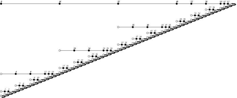
One classical solution used by TAF on the MIT GCM code [14], is called multi level recursive checkpointing. Basically, it splits the complete time interval into a small number of equidistant intervals, then apply the same strategy to each of the sub-intervals. For instance 64 time steps can be split into 4 large intervals of 4 small intervals of 4 time steps, as sketched on figure 3. This consumes a maximum of 9 simultaneous snapshots, and the average number of duplicate executions for a time step is $2.25$. In a more realistic situation, 1000 time steps can be split into 10 large intervals of 10 small intervals of 10 time steps, and one can figure out that this consumes a maximum of 27 simultaneous snapshots, and the average number of duplicate executions for a time step is $2.7$.

Figure 3: Three-levels checkpointing with 64 time steps and 9 snapshots. Forward computations go right, adjoint computations go left. Black circles represent writing/taking a snapshot, white circles represent reading an available snapshot.

However, it was shown in [21] that this strategy is not optimal. Under the reasonable assumptions that all time steps cost the same run time, and that the snapshot needed to run again from time step $n$ to $n+1$ is the same as to run from step $n$ to any later step $n+x$, Griewank and Walther have characterized the optimal distribution of nested checkpoints, which follows a binomial law. With this optimal strategy, both spatial and temporal complexity of the adjoint code grow logarithmically with respect to the number of time steps of the original simulation. In other words, both the slowdown factor which grows like the number of times each time step is executed, and the memory which grows like the number of simultaneous snapshots, grow logarithmically with the total number of time steps.

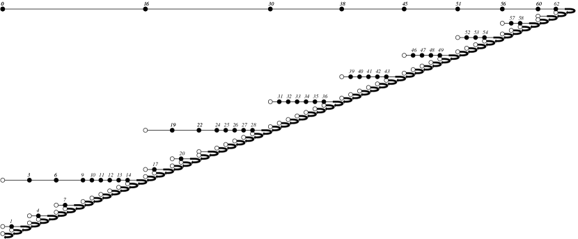
In real applications, run-time and memory space do not behave symmetrically. One can always wait a little longer for the result, whereas the memory space is bounded. Therefore the maximum number of snapshots $d$ that can be stored simultaneously is fixed. Then [8] shows that the optimal strategy gives a slowdown factor that grows only like the $d^{th}$ root of the total number of time steps, which is still very good. Figure 4 shows the optimal checkpointing strategy for the same problem as figure 3 i.e. 64 time steps with memory for 9 snapshots. The average number of duplicate executions for a time step is only $2$. For the more realistic situation (1000 time steps and memory for 27 snapshots) the average number of duplicate executions is only $2.57$.

Figure 4: Optimal binomial checkpointing with 64 time steps and 9 snapshots

We implemented this optimal strategy in the adjoint code of OPA. We made our first experiments by hand modification of the adjoint code produced by TAPENADE. Still, TAPENADE produced automatically the procedures that store and retrieve the snapshot, and therefore the hand modification was benign: given the number of time steps, a general procedure schedules the optimal sequence of actions (store snapshot, retrieve snapshot, run time step, run adjoint time step) to differentiate the complete simulation. Further versions of TAPENADE will fully automate this process. Figure 5 shows the performances on OPA.

Figure 5: Optimal binomial checkpointing with 15 snapshots: slowdown factor as a function of the total length of the initial simulation. The slowdown factor is the run-time ratio of the adjoint code compared to the original code.

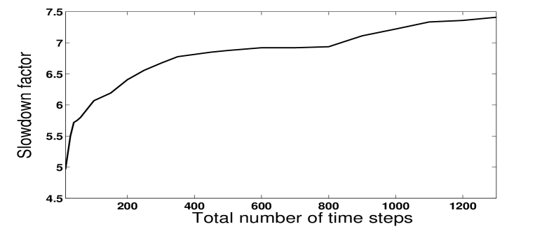
They are in good agreement with the theory. Notice in particular the two small inflection points on the curve around 150 iterations and 800 iterations. Going back to the optimality proof in [8], we see that the optimal strategy is particularly efficient when the number of time steps is exactly

$$\eta(d,t)=\frac{(d+t)!}{d!t!}$$

where $d$ is the number of snapshots and $t$ is the number of duplicate executions allowed per time step. For our target machine $d=15$ and we find $\eta(15,2)=136$ and $\eta(15,3)=816$, which corresponds to the inflection points of figure 5.

For the previous version OPA 8, the adjoint was written by hand. Nevertheless, even a hand-written adjoint must implement strategies to retrieve intermediate states in reverse order that is, something very close to checkpointing. Looking at this hand-written adjoint, we first observe that the checkpointing strategy is neither multi level nor optimal binomial. It is more like a single level strategy, with one snapshot stored every fixed number of time steps. During the reverse sweep, states between two stored snapshots are rebuilt approximately using linear interpolation. The advantage is that few time steps are evaluated twice, and therefore the slowdown factor remains well below 4. We can see at least two drawbacks. First, this hand manipulation requires deep knowledge of the original program and of the underlying equations. This method does not blend easily with Automatic Differentiation. It is not yet automated in any AD tool and therefore tedious and error-prone code manipulations would still be necessary. Second, this introduces approximation errors into the computed derivatives, whose mathematical behavior is unclear. The gradient obtained in the end is used in complex optimizations or data-assimilation loops, and small errors may result in poor convergence. In any case, for very large numbers of time steps, we believe a trade-off between exact binomial checkpointing and approximate interpolation is worth experimenting. Interpolation is probably good enough for many variables that vary very slowly, and which could be designated by the end-user, and only the other variables would need to be stored.

4.4 Iterative linear solver

The OPA model solves an elliptic equation at the end of each time step, using an iterative method that generates a sequence of approximations of the exact solution. The mechanical application of AD on this kind of methods gives a sequence of derivatives of the approximate solutions with the same number of iterations as the original solver. The reason is that AD keeps the flow of control of the original program in the differentiated program. In particular the convergence tests are still based only on the non-differentiated variables. Naturally, one may ask whether and how AD-produced derivatives are reasonable approximations to the desired derivative of the exact solution. The issues of derivative convergence for iterative solvers in relation to AD are discussed in [6, 9, 2].

OPA provides two alternative algorithms to solve the elliptic equation: “PCG” for Preconditioned Conjugate Gradient, and “SOR” for Successive Over-Relaxation method. Both algorithms give correct results for the original code, but PCG is generally preferred thanks to its efficiency and vectorization properties. However, the AD-differentiated code gives different results using the two algorithms. Figure 6 compares the AD-derivatives with approximate derivatives obtained by divided differences. We see that the derivatives obtained with the SOR algorithm remain correct when the number of time steps increases. On the contrary, the derivatives obtained with the PCG algorithm become completely wrong after 80 time steps. Notice that this occurs in tangent mode as well as in adjoint mode: the derivatives obtained with PCG, although wrong, remain identical in tangent and adjoint. Our explanation is that each iteration of PCG involves the computation of scalar products of variables that depend on the state vector, thus making the numerical algorithm nonlinear even though the elliptic equation is linear. In [6], Gilbert has shown that the application of AD to a fixed point iteration gives a derivative fixed point iteration that converges R-linearly to the desired derivative in particular in the case of a large contractive iterate or secant updating. Unfortunately this is not the case for quasi-Newton iterative solvers such as PCG, for which there is no similar convergence result to our knowledge.

Figure 6: evolution of the relative error between tangent derivative and divided differences, for the three strategies: SOR and straightforward AD, PCG and straightforward AD, PCG with the black box strategy

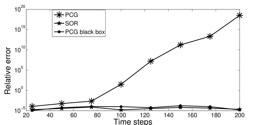
To solve this problem for the tangent-differentiated OPA we exploit the linearity of the elliptic system, and for the adjoint-differentiated OPA we exploit the self adjointness property of the elliptic operator [22]. We can thus use the original PCG routine itself to solve for the differentiated linear systems. Practically, we do this using the so-called “black-box” feature provided in TAPENADE. Figure 6 shows that (here for the tangent mode) the PCG gives the same accuracy as the SOR solver.

In another experiment, we tried to use straightforward AD with the PCG solver, but this time fixing the number of PCG iterations to some very high value. We observed that the derivatives become coherent again with divided differences. This could be another way to solve our problem, but it is certainly expensive and the choice of the “high” iteration number is delicate. This problem definitely deserves further study, and confirms the general recommendation not to differentiate solvers of a nonlinear kind, and use a black-box strategy instead.

5 Validation Experiments

5.1 Correctness test

The classical way to check for correctness of the automatically generated tangent and adjoint codes is as follows:

1. Choose an arbitrary input $X$ and and arbitrary direction $\dot{X}$. Compute the Divided Difference

   $$D\!D=\dfrac{F(X+\varepsilon\dot{X})-F(X)}{\varepsilon}$$

   for a good enough small $\varepsilon$.

2. Using the tangent differentiated program, compute $\dot{Y}=F^{\prime}(X)\times\dot{X}$.

3. Using the adjoint differentiated program, compute $\overline{X}=F^{\prime*}(X)\times\dot{Y}$

and finally check that $(D\!D\cdot D\!D)=(\dot{Y}\cdot\dot{Y})=(\overline{X}\cdot\dot{X})$. We performed this test for the complete global ORCA-2 simulation on 1000 time steps and its derivative codes. The results are shown in table 1. The values match,

Table 1: Dot product test for 1000 time steps

$(D\!D\cdot D\!D)$ ($\varepsilon=10^{-7}$)	4.405352760987440e+08
$(\dot{Y}\cdot\dot{Y})$	4.405346876439977e+08
$(\overline{X}\cdot\dot{X})$	4.405346876439867e+08

and $(\dot{Y}\cdot\dot{Y})$ and $(\overline{X}\cdot\dot{X})$ match very well, up to the last few digits, which shows that the tangent and adjoint codes really compute the same derivatives, only in a different computation order as shown by equations (2) and (3). The values of $(D\!D\cdot D\!D)$ and $(\dot{Y}\cdot\dot{Y})$ don’t match so well, because of the weakness of the Divided Differences approximation.

Figure 7: Relative error of Divided Differences with respect to AD-generated derivatives, computed for various values of of the step size $\varepsilon$

Figure 7 shows this weakness: For a small value of $\varepsilon,$ the dominant error is due to machine accuracy. For a large value of $\varepsilon,$ the dominant error is due to the second derivatives of $F$. The best $\varepsilon$ minimizes both errors, but cannot eliminate them completely.

5.2 Sensitivity analysis on a long simulation

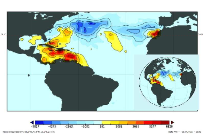
One of the main application of adjoint models is the sensitivity analysis i.e. the study of how model output varies with changes in model inputs. Using direct or statistical methods would require many integration of the non linear model while one adjoint model integration is enough to compute this sensitivity. As an example, figure 8 shows the output map of the sensitivity of the North Atlantic meridional heat flux at 29°N to changes in the initial sea surface temperature ($SST_{t_{0}}$) over one year integration period, starting January 1, 1998. This is done by computing the gradient respect to $SST_{t_{0}}$ of

$$J=\int_{t_{0}}^{t_{N}}\iint_{\Omega}T.v\ dxdzdt$$

where $\Omega$ is the zonal cross section at 29°N in the North Atlantic, $T$ is the temperature and $v$ is the meridional current velocity.

Contours in figure 8 show where variation of initial SST would effect the most upon heat transport at 29°N. It shows large scale patterns mainly located north of the 29°N parallel and in the Caribbean sea with a strong spot off Morocco. These results are consistent with those obtained by Marotzke et al. ([18])

This map was computed by the TAPENADE-generated adjoint of OPA on the global ORCA2 grid, over 5475 time steps (1 year). This experiment was done with the SOR algorithm as the iterative linear solver. The TAPENADE-generated adjoint computed this sensitivity map in a time that is only 8.03 times that of the original simulation.

Figure 8: Sensitivity map of the North Atlantic heat transport at 29°N (dotted line), with respect to changes in the initial surface temperature

5.3 Data Assimilation

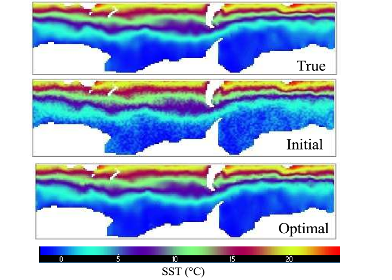
For further validation of the automatically generated derivatives, we carried out a data assimilation experiment. This was done in a so-called twin experiment framework whereby the direct model trajectory is used to generate synthetic observations. The initial sea surface temperature is perturbed by a white noise and it has to be recovered using variational data assimilation techniques. Synthetic observation are given by the sea surface height (SSH) and the sea surface salinity (SSS) generated from the model’s original outputs starting from the unperturbed SST.

The cost function to be minimised is

$$J(SST({t_{0}}))=\int_{t_{0}}^{t_{N}}\parallel SSH(t)-SSH^{o}(t)\parallel^{2}+\parallel SSS(t)-SSS^{o}(t)\parallel^{2}dt$$ (4)

Where the superscript ^o stands for synthetic observation and $SSH(t)$ and $SSS(t)$ are model output.

For computing cost issues, only the Antarctic zoom of ORCA2 is considered, the minimisation is done an iterative gradient search algorithm where the gradient of $J$ is cumputed using adjoint techniques. Figure 9 illustrates the performance of the optimization loop for an integration period of 1 month i.e. 450 time steps. The cost function decreases by two orders of magnitude.

Figure 10 indicates that the true solution (top panel) is recovered with a good approximation (bottom panel) from the randomly perturbed one(middle panel), showing the quality of the derivatives obtained.

Figure 9: Twin experiment: Convergence of the cost function

Figure 10: Twin experiment: True field (top), Initial perturbed field (middle) and identified optimal sea surface temperatures (bottom)

6 Conclusion and Outlook

The effort to build the tangent and adjoint codes for the previous version 8 of the OPA ocean General Circulation Model has cost several months development from an experienced researcher. For the new version OPA 9 written in FORTRAN95, the use of the AD tool TAPENADE significantly reduces this effort. Our first numerical applications show the quality of the derivatives obtained. This works validates the choice of AD as the strategy to obtain the tangent and adjoint for OPA 9, and for the versions to come.

At the same time, OPA is the largest FORTRAN95 application differentiated with TAPENADE. This work has pointed at a number of limitations of TAPENADE that have been lifted. Other limitations remain, such as the non-reentrant procedures, which need to be addressed in future work. Successful differentiation of OPA definitely increases our confidence in TAPENADE.

This works is also an additional illustration of the superiority of the binomial checkpointing strategy, compared to multi level checkpointing. By the standards of other application fields, e.g. CFD, a slowdown of the adjoint code of only 7 for a nonsteady simulation on 1000 time steps would be considered very good. By the standards of weather simulation or ocean modeling however, scientists expect yet faster adjoints, at the cost of a radical approximation. Even if we consider that these approximations change the mathematical nature of the optimization process, we understand they are necessary and we shall study how they can be proposed as an option by the AD tool.

This work has underlined several directions for further research in AD and AD tools. Some of them are already being studied by researchers in our groups. Considering the application language, two constructs need to be differentiated better:

• The next experiment to be made very soon is to apply TAPENADE to the parallelized version of OPA. This is necessary before the generated tangent and adjoint codes can be used in production context.

• The OPA source makes extensive use of the preprocessor directives such as #IFDEF. TAPENADE does not deal with these directives because they do not respect the syntactic structure of a code. Handling these directives in the AD tool is in our opinion hopeless. What might be done though, is to generate differentiated codes for each possible preprocessed code, and devise a tool to put the directives back into the differentiated codes. This is made easier if the differentiated code closely follows the structure of the original, as is the case with TAPENADE.

Considering specifically adjoint differentiation, we hope to obtain more efficient code through a more systematic exploitation of self-adjointness, e.g. of the elliptic operator. We also hope to optimize the checkpointing strategy. In its present version, TAPENADE applies checkpointing to each procedure call. Using profiling information, we believe we can detect several procedure calls for which checkpointing is useless or counter-productive. TAPENADE is already able to use this information to produce a better adjoint.

References

- [1] W. Castaings, D. Dartus, M. Honnorat, F.-X. Le Dimet, Y. Loukili, and J. Monnier. Automatic differentiation: A tool for variational data assimilation and adjoint sensitivity analysis for flood modeling. In Bücker et al, editor, Automatic Differentiation: Applications, Theory, and Implementations, LNCSE, pages 249–262. Springer, 2005.
- [2] B. Christianson. Reverse accumulation and attractive fixed points. Optimization Methods and Software, 3:311–326, 1994.
- [3] P. Courtier, J.-N. Thépaut, and A. Hollingsworth. A strategy for operational implementation of 4d-var, using an incremental approach. Q. J. R. Meteorol. Soc., 120:1367–1387, 1994.
- [4] R. Giering. Tangent linear and Adjoint Model Compiler, Users manual, 1997. http://www.autodiff.com/tamc.
- [5] R. Giering and T. Kaminski. Recipes for adjoint code construction. ACM Transactions on Mathematical Software, 24(4):437–474, 1998.
- [6] J.C. Gilbert. Automatic differentiation and iterative processes. Optimization Methods and Software, 1:13–21, 1992.
- [7] M.B. Giles, D. Ghate, and M.C. Duta. Using automatic differentiation for adjoint CFD code development. In Uthup et al, editor, Recent Trends in Aerospace Design and Optimization, pages 363–373. Tata-McGraw Hill, New Delhi, 2005. Post-SAROD-2005, Bangalore, India.
- [8] A. Griewank. Achieving logarithmic growth of temporal and spatial complexity in reverse automatic differentiation. Optimization Methods and Software, 1:35–54, 1992.
- [9] A. Griewank, C. Bischof, G. Corliss, A. Carle, and K. Williamson. Derivative convergence for iterative equation solvers. Optimization Methods and Software, 2:321–355, 1993.
- [10] A. Griewank, D. Juedes, J. Srinivasan, and C. Tyner. ADOL-C, a package for the automatic differentiation of algorithms written in C/C++. ACM Trans. Math. Software, 22(2):131–167, 1996.
- [11] L. Hascoët and M. Araya-Polo. The adjoint data-flow analyses: Formalization, properties, and applications. In Automatic Differentiation: Applications, Theory, and Tools, Lecture Notes in Computational Science and Engineering. Springer, 2005. Selected papers from AD2004 Chicago.
- [12] L. Hascoët and V. Pascual. Tapenade 2.1 user’s guide. Technical Report 0300, INRIA, 2004.
- [13] L. Hascoët, M. Vázquez, and A. Dervieux. Automatic differentiation for optimum design, applied to sonic boom reduction. In Kumar et al., editor, Proceedings of ICCSA’03, Montreal, Canada, pages 85–94. LNCS 2668, Springer, 2003.
- [14] Heimbach, P. and Hill, C. and Giering, R. An efficient exact adjoint of the parallel MIT general circulation model, generated via automatic differentiation. Future Generation Computer Systems, 21(8):1356–1371, 2005.
- [15] J. Kim, E. Hunke, and W. Lipscomb. Sensitivity analysis and parameter tuning scheme for global sea-ice modeling. Ocean Modeling Journal, 14(1–2):61–80, 2006.
- [16] C. Lauvernet, F. Baret, L. Hascoët, and F.-X. LeDimet. Improved estimates of vegetation biophysical variables from meris toa images by using spatial and temporal constraints. In proceedings of the 9th ISPMSRS, Beijing, China, 2005.
- [17] G. Madec, P. Delecluse, M. Imbard, and C. Levy. Opa8.1 ocean general circulation model reference manual. Technical report, Pole de Modelisation, IPSL, 1998.
- [18] J. Marotzke, R. Giering, K.Q. Zhang, D. Stammer, C. Hill, and T. Lee. Construction of the adjoint MIT ocean General Circulation Model and application to atlantic heat transport sensitivity. J. Geophys. Res., (104(C12)):29,529–29,548, 1999.
- [19] O. Talagrand. The use of adjoint equations in numerical modeling of the atmospheric circulation. In A. Griewank and G. Corliss, editors, Automatic Differentiation of Algorithms: Theory, Implementation and Application, pages 169–180, 1991. Philadelphia, Penn: SIAM.
- [20] J. Utke, U. Naumann, M. Fagan, N. Tallent, Strout M., P. Heimbach, C. Hill, and C. Wunsch. OpenAD/F: A modular, open-source tool for Automatic Differentiation of Fortran codes. Technical report ANL/MCS-P1230-0205, Argonne National Laboratory, 2006. Submitted to ACM TOMS.
- [21] A. Walther and A. Griewank. Advantages of binomial checkpointing for memory-reduced adjoint calculations. In Feistauer et al, editor, Numerical Mathematics and Advanced Applications, pages 834–843. Springer, Berlin, 2003. Proceeding of ENUMATH 2003.
- [22] A. Weaver, J. Vialard, and D. Anderson. Three- and four-dimensional variational assimilation with an ocean general circulation model of the tropical pacific ocean: I. formulation, internal diagnostics and consistency checks. Monthly Weather Review, 131(7):1360–1378, 2003.