Detecting the rise and fall of 21 cm fluctuations with the Murchison Widefield Array
Abstract
We forecast the sensitivity with which the Murchison Widefield Array (MWA) can measure the 21 cm power spectrum of cosmic hydrogen, using radiative transfer simulations to model reionization and the 21 cm signal. The MWA is sensitive to roughly a decade in scale (wavenumbers of Mpc-1), with foreground contamination precluding measurements on larger scales, and thermal detector noise limiting the small scale sensitivity. This amounts primarily to constraints on two numbers: the amplitude and slope of the 21 cm power spectrum on the scales probed. We find, however, that the redshift evolution in these quantities can yield important information about reionization. We examine a range of theoretical models, spanning plausible uncertainties in the nature of the ionizing sources, and the abundance of gas-rich mini-halos during reionization. Although the 21 cm power spectrum differs substantially among these models, a generic prediction is that the amplitude of the 21 cm power spectrum on MWA scales ( Mpc-1) peaks near the epoch when the intergalactic medium (IGM) is ionized. Moreover, the slope of the 21 cm power spectrum on MWA scales flattens as the ionization fraction increases and the sizes of the HII regions grow. Considering detection sensitivity, we show that the optimal MWA antenna configuration for power spectrum measurements would pack all antenna tiles as close as possible in a compact core. Provided reionization occurs in the MWA observing band, this instrument is sensitive enough in its optimal configuration to measure redshift evolution in the slope and amplitude of the 21 cm power spectrum. Detecting the characteristic redshift evolution of our models will help confirm that observed 21 cm fluctuations originate from the IGM, and not from foregrounds, and will provide an indirect constraint on the evolution of the volume-filling factor of HII regions during reionization. After two years of observations under favorable conditions, the MWA can constrain the filling factor at an epoch when to within roughly at confidence. It can also constrain models for the ionizing sources and the abundance of mini-halos during reionization.
Subject headings:
cosmology: theory – intergalactic medium – reionization – large scale structure of universe1. Introduction
Detecting 21 cm emission from the high redshift IGM will provide fully three-dimensional information on the epoch of reionization (EoR). Futuristic experiments like the Square Kilometer Array (SKA) will have the sensitivity to produce maps of reionization as a function of redshift (Zaldarriaga et al. 2004, McQuinn et al. 2006). These maps, taken in various frequency bands and with sufficiently high angular resolution, will amount to a reionization ‘movie’: they will depict the growth of HII regions around individual sources and their subsequent mergers with neighboring HII regions, and detail the completion of the reionization epoch, whereby the entire volume of the Universe becomes filled with ionized hydrogen.
While producing a reionization movie is perhaps the ultimate goal of 21 cm studies, first generation surveys like the MWA111The array formerly known as the Mileura Widefield Array, is now known as the Murchison Widefield Array, owing to a change of site. will already provide valuable insights into the reionization process. These first generation surveys will lack the sensitivity required to produce detailed maps, but will allow for a statistical detection. For example, the MWA is expected to measure the power spectrum of 21 cm brightness temperature fluctuations over roughly a decade in scale, in each of several redshift bins (McQuinn et al. 2006, Bowman et al. 2006).
In this paper, we use radiative transfer simulations (Sokasian et al. 2001, 2003, Zahn et al. 2007, McQuinn et al. 2007a, 2007b) to quantify how well power spectrum measurements with the MWA can constrain the reionization process. How well can we deduce the gross features of the reionization movie from a statistical detection? In particular, we aim to check whether the MWA can constrain the volume filling factor of HII regions as a function of time. Reliable estimates of the volume filling factor of HII regions – the ‘ionization fraction’ of the IGM – will pinpoint the timing and duration of reionization. This information, marking a key event in the formation of structure in our universe, will constrain models for the ionizing sources, and solidify existing measurements from cosmic microwave background (CMB) polarization (Page et al. 2007), quasar spectra (Fan et al. 2006, Lidz et al. 2006, 2007a, Becker et al. 2007, Bolton & Haehnelt 2007a, 2007b, Mesinger & Haiman 2007, Wyithe et al. 2005, Wyithe et al. 2007, Gallerani et al. 2007), Ly- emitter (LAE) surveys (Malhotra & Rhoads 2005, Kashikawa et al. 2006, Furlanetto et al. 2006c, Dijkstra et al. 2007, McQuinn et al. 2007b, Mesinger & Furlanetto 2007a), and gamma-ray burst (GRB) optical afterglow spectra (Totani et al. 2006, McQuinn et al. 2007c.), which currently provide tantalizing, yet controversial and subtle to interpret, clues.
The outline of this paper is as follows. In §2 we describe our radiative transfer simulations, and examine the simulated 21 cm power spectrum and its redshift evolution. In §3 we forecast the sensitivity with which the MWA can measure the 21 cm power spectrum, paying attention to foreground contamination, and examining how the sensitivity depends on the, as yet unfinalized, configuration of the MWA’s antenna tiles (§3.3). In §4 we show that the MWA sensitivity generally boils down to constraints on each of the slope and amplitude of the 21 cm power spectrum at Mpc-1. We then quantify how well the MWA can constrain these two numbers in different redshift bins. In §5, we show how constraints on the slope and amplitude of the 21 cm power spectrum in several redshift bins translate into constraints on the redshift evolution of the volume-filling factor of HII regions during reionization. In §6 we summarize our main results and discuss future research directions.
Throughout we consider a CDM cosmology parameterized by: , , , , , and , (all symbols have their usual meanings), consistent with the results from Spergel et al. (2007).
2. The Redshift Evolution of the 21 cm Power Spectrum
In this section, we examine the redshift evolution of the 21 cm power spectrum using the radiative transfer simulations of McQuinn et al. (2007a, 2007b). We focus on the power spectrum since the MWA is expected to have limited imaging sensitivity, but can still provide a statistical detection of 21 cm fluctuations. First, let us briefly define terms. In the limit that the spin temperature of the 21 cm transition, , is globally much larger than the CMB temperature, , and ignoring peculiar velocities, the 21 cm brightness temperature relative to the CMB at spatial position is:
| (1) |
Here, is the 21 cm brightness temperature, relative to the CMB temperature, at redshift and frequency MHz, for a neutral gas element at the cosmic mean gas density; mK in our adopted cosmology (Zaldarriaga et al. 2004). The quantity is the volume-averaged neutral fraction, is the fractional fluctuation in neutral fraction, while is the fractional gas density fluctuation. We frequently quote results in terms of the volume-averaged ionization fraction, , rather than in terms of the neutral fraction.
In general, we measure the power spectrum of and plot the dimensionless power spectrum of this dimensionless quantity, – i.e, we plot the variance per logarithmic interval in wavenumber of the field . We ignore peculiar velocities throughout since they have little impact during the bulk of the reionization epoch when ionization fluctuations are large (McQuinn et al. 2006, Mesinger & Furlanetto 2007b). We consider only spherically-averaged power spectra since the MWA has limited sensitivity in the transverse direction (McQuinn et al. 2006).
2.1. Radiative Transfer Simulations
Let us briefly describe the simulations used in our analysis, and our fiducial model for the ionizing sources and reionization history. Radiative transfer is post-processed on an evolved N-body simulation using the code of McQuinn et al. (2007a), a refinement of the Sokasian et al. (2001, 2003) code, which in turn uses the adaptive ray-tracing scheme of Abel & Wandelt (2002). Some other approaches to large scale reionization simulations are described in Iliev et al. (2006), Kohler et al. (2005), Trac & Cen (2006) and Croft & Altay (2007). The radiative transfer calculation is performed on top of a Mpc/, particle dark matter simulation run with an enhanced version of Gadget-2 (Springel 2005). The minimum resolved halo in this simulation is , but smaller mass halos down to the atomic cooling mass (Barkana & Loeb 2001), , are incorporated with the appropriate statistical properties as in McQuinn et al. (2007a). Ionizing sources are placed in simulated halos with simple prescriptions. In our fiducial model, we assume that a source’s ionizing luminosity is proportional to its host halo mass. More specifically, our fiducial model is similar to the ‘S1’ simulation of McQuinn et al. (2007a), except that our model here was run in a slightly different cosmology, and in a larger ( Mpc/ rather than Mpc/) simulation box. Additionally, the radiative transfer calculations (and our subsequent power spectrum measurements) are computed on a grid, rather than a grid.
As we show subsequently, the MWA’s ability to detect the 21 cm signal from reionization depends strongly on the timing and duration of this process (McQuinn et al. 2006, Bowman et al. 2006). Presently, we are unable to predict reliably when reionization occurs, and how long it lasts. This depends on many poorly constrained factors such as the efficiency and initial mass function of star formation at high redshift, the clumpiness of the high redshift IGM, the escape fraction of ionizing photons from host galaxies, the degree to which photoionizing and supernova feedback suppress star formation in low mass galaxies, and other uncertain physics (see, e.g., the review by Furlanetto et al. 2006a). In our fiducial model, reionization commences around , at which point of the volume of the IGM is ionized, with of the volume ionized by , by , and by . The reionization epoch may easily occur at significantly different redshifts than in this model and likely satisfy all existing constraints mentioned in the introduction, i.e., from CMB polarization, quasar spectra, LAE surveys, and the optical afterglow spectra of GRBs.
However, our predictions for the power spectrum of ionization fluctuations at a given ionization fraction are more robust than our predictions at a given redshift, which suffer from the large uncertainties noted above. In particular, McQuinn et al. (2007a) demonstrated that the ionization power spectrum varies weakly with redshift when considered in a given model at fixed ionization fraction, a consequence of the fact that, in most plausible models, the bias of the ionizing sources is a weak function of redshift (Furlanetto et al. 2006b). The 21 cm power spectrum depends somewhat more strongly on redshift at fixed ionization fraction than the ionization power spectrum, since the 21 cm field explicitly involves the density field, which evolves in time. Nevertheless, this dependence is relatively weak during most of the EoR when the ionization fluctuations are large (§2.3), and one can think of our predictions in a given model as roughly invariant with redshift for a given ionization fraction. Moreover, we aim to extract information regarding the filling factor of HII regions from the observations, so it will be convenient to consider the signal as a function of this quantity. Of course, as we noted earlier, the uncertain mapping between ionization fraction and redshift can strongly impact the detectability of the signal (§3).
2.2. Simulated Power Spectrum in our Fiducial Model
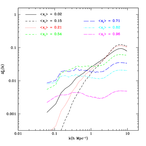
In Figure 1, we show the spherically-averaged 21 cm power spectrum from our fiducial model for a range of redshifts and ionization fractions. At early times and low ionization fraction (, ), the 21 cm power spectrum simply traces the density power spectrum, except on very small scales where early HII regions have some impact. At slightly later times, there is a brief phase (at ) where the large-scale 21 cm power spectrum falls below the density power spectrum, and steepens in slope. This occurs because the large-scale overdense regions initially contain more neutral hydrogen than underdense ones, and consequently appear brighter in 21 cm. On the other hand, the overdense regions ionize first, and quickly transition to being dimmer in 21 cm than underdense ones, which remain neutral. This transition leads to a brief ‘equilibration’ phase where overdense and underdense regions have similar brightness temperatures, and the large-scale 21 cm power spectrum is low as a result (Furlanetto et al. 2004, Wyithe & Morales 2007). At these early stages of reionization, however, our calculations may be inaccurate since we neglect the impact of spin temperature fluctuations (Pritchard & Furlanetto 2007).
After the brief equilibration phase, the HII regions quickly grow, boosting the large-scale power spectrum and suppressing the power on small scales. As we demonstrate in the next section, the wavenumbers relevant for the MWA are Mpc-1. On these scales, the amplitude of the 21 cm power spectrum rises rapidly from when the filling factor of ionized regions is to when , and then drops off at higher ionized fractions, falling rather quickly when . In conjunction with the increased power, the slope flattens and is close to for .
Provided that there are substantial ionization fluctuations on the scales that the MWA is sensitive to, it is unsurprising that the 21 cm power spectrum amplitude peaks around the epoch in which the IGM is ionized. Recall that the variance in the ionization field averaged on small scales, , must reduce to in the limit that each pixel is either completely neutral or completely ionized. In this limit, the variance in the ionization field peaks when , close to the ionization fraction at which the 21 cm power spectrum reaches its maximum on MWA scales. Of course the 21 cm power spectrum is more complicated, since it depends on the cross-correlation between ionization and overdensity and higher order contributions (Lidz et al. 2007b), and since a large portion of the ionization variance comes from scales that are not probed by the MWA. Nevertheless, our simple argument motivates why the maximum in fluctuation amplitude occurs near .
In summary, although the MWA may be limited to measuring the power spectrum over a decade in scale, our model 21 cm power spectra evolve considerably with redshift and ionization fraction over this range. Hence, sensitivity only to a decade in scale may still be quite valuable, provided the MWA can make measurements over a number of redshift intervals.
2.3. Model Dependence
How robust to model uncertainties is the rise and fall in 21 cm power spectrum amplitude, and the flattening in power spectrum slope, at increasing ionization fraction? In order to check this, we examine the amplitude and slope of the 21 cm power spectrum for two other cases that roughly bracket model uncertainties. McQuinn et al. (2007a) investigated the many uncertain physical parameters that can impact reionization and found that the nature of the ionizing sources and the abundance of mini-halos have the strongest influence on the ionization power spectrum. If the sources are rare but very luminous and lie predominantly in rather massive halos, then the high clustering of the ionizing sources leads to larger HII regions at a given ionization fraction, and the ionization power spectrum is peaked on larger scales than in our fiducial model. On the other hand, if mini-halos are abundant, the HII regions are smaller, and the ionization power spectrum is peaked on smaller scales than in our fiducial model (Furlanetto & Oh 2005, McQuinn et al. 2007a). The cross-correlation between ionization and overdensity is also less significant with rare, efficient sources, which acts in conjunction with the increased ionization power in these models to boost the 21 cm power spectrum relative to our fiducial model (Lidz et al. 2007b).
As a representative case with rare sources and large bubbles, we use a model similar to ‘S3’ of McQuinn et al. (2007a), except run in our present larger volume. Briefly, the S3 model has source luminosity : hence, the most massive, highly clustered halos produce most of the ionizing photons. Our representative case with abundant mini-halos and small bubbles, adds mini-halos of dark matter halo mass into the simulation with the appropriate statistical properties (McQuinn et al. 2007a). Each mini-halo is given a cross section to ionizing photons initially equal to its halo virial radius and we subsequently assume that each mini-halo is photo-evaporated on a sound-crossing time. This is a relatively extreme situation since in reality the mini-halo cross sections will shrink with time before they become completely photo-evaporated (Shapiro et al. 2004, Iliev et al. 2005), and since many mini-halos may be photo-evaporated by pre-heating prior to reionization (Oh & Haiman 2003).
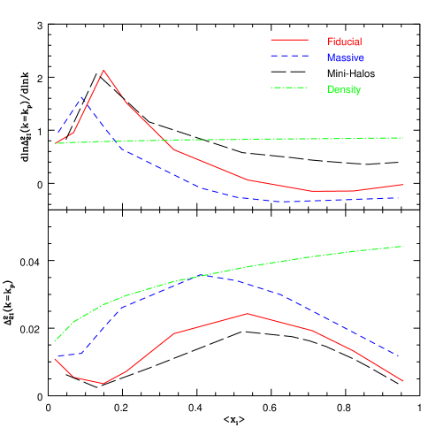
We then determine the amplitude and slope of the 21 cm power spectrum in each model, and plot these quantities as a function of ionization fraction. The results of this calculation are shown in Figure 2. As a convenient choice, we consider the amplitude and slope of the 21 cm power spectrum at a wavenumber Mpc-1, which is close to the middle of the range of wavenumbers probed by the MWA (see §4). We refer to call this as the ‘pivot wavenumber’ since we center our power law fits in §4 on this value.
Concentrating first on the bottom panel of Figure 2, it is clear that the 21 cm power spectrum amplitude at fixed ionization fraction differs significantly among the different cases. The rare source model has the largest amplitude fluctuations, the mini-halo model the smallest ones, and our fiducial model has an intermediate level of fluctuations – precisely the trends anticipated above. Note that, despite the presence of ionization fluctuations, the amplitude of the 21 cm power spectrum at the pivot wavenumber is generally less than that of the density power spectrum in our models. This is a consequence of the ionization-density cross correlation and higher order terms (Lidz et al. 2007b). However, the relative amplitudes of the 21 cm power spectrum and the density power spectrum are somewhat sensitive to the choice of pivot wavenumber. The density power spectrum falls off more rapidly than the 21 cm power spectrum towards large scales, and hence the 21 cm power spectrum becomes larger than the density power spectrum for smaller wavenumbers (see Figure 1). The basic trend of 21 cm amplitude with redshift or ionization fraction, however, is similar for most wavenumbers within the MWA band.
Although the signal differs significantly between models, the 21 cm power spectrum amplitude rises and falls with increasing ionization fraction in each case. The slight dip in power spectrum amplitude near ionized fraction owes to the equilibration phase discussed earlier. Each model reaches a maximum amplitude rather close to an ionization fraction of , although the maximum in the massive source model occurs at a slightly lower ionization fraction, . The basic trend is very encouraging: the redshift at which the 21 cm power spectrum reaches its maximum may provide an observational signature of the redshift at which the IGM is ionized. The ionization fraction at which the 21 cm power spectrum amplitude reaches a maximum depends somewhat on our choice of pivot wavenumber (see Figure 1), although results are similar near the middle of the range of wavenumbers probed by the MWA. 222Wyithe & Morales (2007) find that the variance of the 21 cm field, smoothed with a cylindrical top-hat of angular scale, reaches a minimum around . This angular scale corresponds to Mpc/ and Mpc-1 at in our cosmology, (although there is some ambiguity in the proportionality factor relating and ). Their cylindrical filter will pass fluctuations on still larger scales, and so this is not necessarily in contradiction with our results which find that the power spectrum on somewhat smaller scales is maximal near . The disadvantage of their approach is that foreground cleaning will prohibit measuring the large-scale modes passed by their cylindrical filter. Their calculation methodology is also accurate on scales only much larger then the sizes of individual HII regions, which may impact their predictions during the middle phase of reionization when HII regions are already quite large.
Let us now turn our attention to our model predictions for the slope of the 21 cm power spectrum on MWA scales, shown in the top panel of Figure 2. In our fiducial model, the 21 cm power spectrum is rather flat with at the end of reionization. This is in contrast to the density power spectrum, which has a slope of near our pivot wavenumber. A similar flattening is seen in the massive source case, but here the flattening occurs at smaller ionization fraction since this model produces large ionized regions even at rather low ionization fractions. The slope of the power spectrum even goes slightly negative after of the volume is ionized. On the other hand, in our mini-halo model, the ionized regions are smaller at a given ionization fraction, and there is consequently less flattening with increasing ionization fraction. The slight steepening seen at early times in our models, near , again owes to the equilibration phase discussed in the previous section.
If the MWA finds that the slope of the power spectrum is significantly flatter than that of the density power spectrum, this immediately argues for the presence of large ionized regions, and implies that reionization is well underway, while detecting fluctuations at all clearly implies that less than of the IGM volume is ionized.333Recently, Wyithe & Loeb (2007) pointed out that neutral gas in damped Ly- (DLA) absorbers will produce a 21 cm signal even after essentially the entire volume of the IGM is reionized. This signal will likely become comparable in amplitude to that from the diffuse IGM only at the very end of reionization and can potentially be distinguished from the diffuse IGM on the basis of its power spectrum shape. Specifically, we expect the DLA contribution to the 21 cm power spectrum to have the form , where is the mass-averaged neutral gas fraction locked up in DLAs, is the mass-averaged DLA bias, and is the matter power spectrum. For plausible numbers of , and , the DLA contribution is a factor of smaller than the diffuse IGM contribution in our fiducial model at and Mpc-1. The diffuse component is even more dominant at large scales, and less dominant on smaller scales. Hence, we expect the DLA contribution to kick in essentially after reionization. The MWA should therefore be able to study each of these interesting signals separately. In the mini-halo model, there is less steepening, and hence detecting a relatively steep 21 cm power spectrum slope by itself does not imply that one is probing an early phase of reionization, as it would for our other cases. It is clear from Figure 2, however, that combining measurements of the 21 cm power spectrum amplitude and slope in a few conveniently placed redshift bins will help move beyond a mere detection of 21 cm fluctuations and allow constraints, albeit indirect ones, to be placed on the ionization fraction as a function of time.
Moreover, given the observational challenges anticipated for 21 cm observations and the possibility that undesirable residuals survive the foreground cleaning process, simple theoretical diagnostics such as the ones mentioned here are extremely valuable. Observing the power spectrum amplitude rise and fall with redshift, and the power spectrum slope flatten, is characteristic of the anticipated reionization signal, but foreground residuals are unlikely to mimic this behavior.
3. MWA Power Spectrum Sensitivity
We now consider the statistical significance at which the MWA might detect this characteristic redshift evolution in the 21 cm power spectrum. We first write down the equations describing statistical error estimates for the 21 cm power spectrum (Zaldarriaga et al. 2004, Morales 2005, McQuinn et al. 2006). We generally follow the notation of Furlanetto & Lidz (2007).
The variance of a 21 cm power spectrum estimate for a single k-mode with line of sight component , restricting ourselves to modes in the upper-half plane, considering both sample variance and thermal detector noise, and assuming Gaussian statistics, is given by:
| (2) |
The first term in Equation (2) is the contribution from sample variance, while the second term comes from thermal noise in the radio telescope. The thermal noise term depends on the system temperature, , the co-moving distance to the center of the survey at redshift , , the survey depth, , the observed wavelength, , the effective area of each antenna tile, , the survey bandwidth, , the total observing time, , and the distribution of antennae. The dependence on antenna configuration is encoded in which denotes the number density of baselines observing a mode with transverse wavenumber (McQuinn et al. 2006). The factor of in the noise term is appropriate because we consider the error in the power spectrum of (Equation 1).
In order to estimate the variance of the power spectrum averaged over a spherical shell of logarithmic width , we add the statistical error for individual -mode estimates in inverse quadrature:
| (3) |
In this equation, denotes the effective survey volume of our radio telescope, and the sum is over all modes in the upper half plane contained within the survey volume. The maximum included in the sum over modes is set by the survey depth, up to a maximum possible of , while the minimum depends on the highest transverse wavenumber sampled by the array, down to a minimum possible of . In practice, we approximate this sum by an integral. We generally plot the error in which is related to the above by a factor of .
Making the array more compact increases the number density of baselines, , sampling low , but truncates the sum over modes (Equation 3) at larger . An important point to note is that, owing to high- line of sight modes in the sum of Equation (3), the MWA can still estimate the power spectrum for wavenumbers with , where is the highest transverse wavenumber probed by the antenna array. Indeed, for the rather compact array configurations expected for the MWA, the sensitivity is concentrated along the line of sight, and the sum over in Equation (3) is restricted to a limited range close to for high modes.
3.1. Assumed MWA Survey Parameters
The MWA will be an array of antenna tiles observing a wide field on the sky of deg2 at frequencies of MHz, corresponding to 21 cm emission redshifts of . Each antenna tile consists of dual polarization dipoles layed out in a m-by- m grid, and covers an effective collecting area of m2 at (Bowman et al. 2006). We linearly interpolate between the values of effective area given in Table 2 of Bowman et al. (2006) to determine the effective antenna areas at other redshifts. We assume that the system temperature is set by the sky temperature, which we take to be K, following Wyithe & Morales (2007). We consider observations over a bandwidth of MHz, and a total observing time of hrs. This integration time represents an optimistic estimate for the total amount of usable observing time the MWA might achieve within a single calendar year. The bandwidth is chosen to be small enough to ensure that the signal evolves minimally over the corresponding redshift interval (McQuinn et al. 2006), which is only at .
We will consider two choices for the antenna distribution, since the sensitivity of the array depends strongly on the configuration of the tiles (McQuinn et al. 2006, Bowman et al. 2006, §3.3). In the first configuration, following Bowman et al. (2006), we assume that a fraction of the antenna tiles are packed as close as physically possible within a m core, and that the remaining antennae follow an distribution out to a maximum baseline of km. This configuration has antennae in the compact m core. In addition, we consider a configuration where all antennae are packed as close as physically possible within a m core, which we will term the ‘super-core’ distribution. For each configuration, we calculate the approximate number density of baselines observing a given transverse mode, , by determining the auto-correlation function of the antenna distribution. In practice, one may not be able to place the antennae as close as physically possible, since, e.g., the tiles will interfere with one another when packed too tightly. Nevertheless, our examples represent useful models to understand how sensitivity depends on array configuration.
3.2. Results
We estimate the statistical error bars from our fiducial model 21 cm power spectrum calculations (Figure 1), using the MWA survey specifications, and Equations (2) and (3), and considering spherical shells of logarithmic width . Note that our hypothetical surveys extend to much higher wavenumbers along than transverse to the line of sight, and so our surveys do not sample full spherical shells in -space at high wavenumber – they only sample a limited fraction of a -space shell close to the line of sight axis.
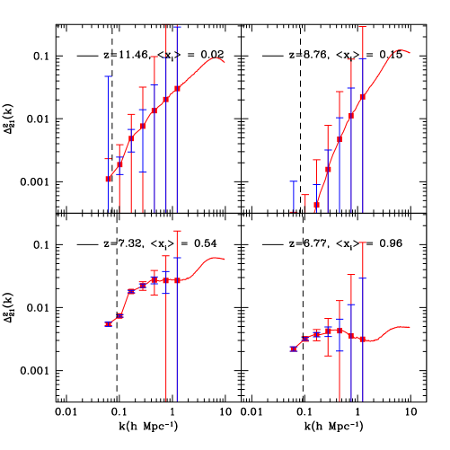
In this section, our calculations are similar to previous work (McQuinn et al. 2006, Bowman et al. 2006), except here we consider a more realistic model for the 21 cm power spectrum. The results of these calculations are shown in Figure 3 for four example redshifts and ionized fractions. The dashed lines in the figure indicate wavenumbers below which foreground removal – for our particular choice of bandwidth, MHz – will prohibit power spectrum measurements. The foreground cleaning process exploits the expectation that the foregrounds are spectrally smooth, while the signal has structure in frequency space (e.g. Zaldarriaga et al. 2004, Morales & Hewitt 2004, Morales et al. 2006, McQuinn et al. 2006). This process will – at the very minimum – remove all line of sight modes with . The discreteness of modes in the survey then implies that all modes with will be lost in the foreground cleaning process. At high wavenumber, the antenna array samples modes poorly owing to its limited angular resolution, and hence power measurements at wavenumber above Mpc-1 are quire noisy.
Measurements early in the EoR generally have low signal to noise. This is illustrated in the top two panels of Figure 3. The sensitivity of the measurements degrades significantly towards high redshift because of the increasing sky brightness towards low frequency, , and because the signal is weaker on large scales at early times. In this particular model, the , measurement actually has less signal to noise than the higher redshift , model. This is because the output is near the equilibration phase (see §2.2), where the large scale power actually drops below the density power spectrum. At lower redshifts, during the intermediate phase of reionization, the MWA will make highly significant power spectrum measurements over a range in scales, as illustrated by the lower left panel where . Indeed, even when the IGM is ionized at in this model, 21 cm fluctuations should be detectable with the MWA in its arrangement, with a strong detection expected for the super-core configuration.
To provide a quantitative measure, we calculate the total at which the MWA can measure the 21 cm power spectrum. We compute the total by taking the square root of the sum of the squares of the in each -bin. For our antenna configuration, this calculation gives , and at and respectively. In the super-core configuration, these numbers are boosted to and respectively. Taken at face value, these numbers imply that the MWA, in its super-core configuration, can achieve a power spectrum detection when the IGM is neutral after only hrs of integration time. Note, however, that most of the detection sensitivity comes from the first -bin beyond the foreground limit. Given that this first bin is potentially most impacted by residual foregrounds (McQuinn et al. 2006), and given that the discriminating power between models is slightly larger at higher , we also quote the at which one can measure power in the -bin with Mpc-1 (and ), near the middle of the range of scales probed by the MWA. In the super-core configuration, the for detecting power in this -bin is , and for the respective above (see also §4).
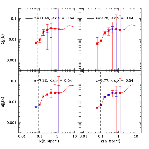
To get a sense for how the power spectrum signal to noise depends on when reionization occurs, we repeat our sensitivity calculations for models in which at each of and . We contrast these models with our earlier calculations in which at these respective redshifts. In order to avoid running additional radiative transfer calculations, we construct 21 cm fields at these redshifts using in each case the ionization field in our fiducial model at (which has ), in conjunction with the simulated density field at each desired redshift. This should be a good approximation since the ionization power in a given model depends mainly on the ionization fraction and not explicitly on redshift (McQuinn et al. 2007a).
The results of this calculation are shown in Figure 4. Comparing with the results of Figure 3, we see that the 21 cm power spectrum sensitivity at a given redshift is enhanced significantly when compared to the sensitivity at the beginning or end of reionization. The large ionized bubbles during the middle phase of reionization significantly boost the amplitude of the 21 cm power spectrum on large scales, and facilitate detection above the thermal detector noise. Quantitatively, the total at which the MWA can detect the 21 cm power spectrum at in our fiducial model (in which case ) is only for the antenna configuration, and for the super-core distribution. If at this redshift, however, the increases to in the configuration, and for the super-core arrangement. For comparison, the at which the MWA can detect power in the Mpc-1 bin is and when at , and respectively. Interestingly, despite the increased sky noise towards high redshift, the MWA can still expect a detection at if at this redshift.
It is also interesting to examine how strong a lower limit on the ionization fraction the MWA might place from a null detection. If the IGM is mostly ionized at , for example, should we expect the MWA to detect 21 cm power at this redshift? To investigate this, we use the ionization fields from our fiducial model at to produce mostly ionized 21 cm power spectrum models at . Interestingly, with our fiducial survey parameters these models both yield power spectrum detections in each of the and super-core configurations, provided we include all modes with wavenumber larger than our foreground cut. For comparison, the for detecting power in the Mpc-1 bin alone is larger than only for the model in the super-core configuration. The super-core configuration produces only a power spectrum detection in this bin at , , while neither model produces a significant detection in this bin with the antenna configuration. Hence if the MWA fails to detect power at , this will still provide a stringent lower limit on . Since much of the power spectrum sensitivity comes from -bins close to the foreground limit, however, the precise lower limit depends on how well foreground cleaning algorithms perform for wavenumbers close to the foreground cut (McQuinn et al. 2006). This is an important topic for further study.
3.3. Sensitivity to Array Configuration
As noted earlier (Zaldarriaga 2004, McQuinn et al. 2006, Bowman et al. 2006), the sensitivity of 21 cm power spectrum measurements depends strongly on the array’s antenna tile configuration. Here we expand on this point, advocating a still more compact antenna distribution than previous authors.
Concentrating on the fiducial model output at where the of the detection is highest, it is clear that the super-core configuration yields significantly smaller statistical error bars. At Mpc-1 the statistical error bars are a factor of smaller in the super-core configuration than for the distribution, but by Mpc-1, the error bars are a factor of smaller in the super-core configuration. The gain in sensitivity at low is less substantial because the large scale modes become sample variance dominated, and hence making the array more compact beyond some point does not further boost power spectrum sensitivity. Interestingly, the fact that large scale modes become sample variance dominated in the super-core configuration, implies that the MWA is capable of imaging large scales modes in this arrangement – i.e., the signal to noise per mode is unity for some large scale modes. We will consider the MWA’s imaging capabilities in future work. Here we focus on the array’s sensitivity for statistical power spectrum measurements.
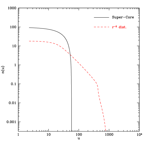
The increased sensitivity of the array in its compact core configuration arises because the long baselines in the distribution are too sparsely sampled to be useful. To illustrate this, we plot the number density of baselines observing a given visibility (see Equation 2) for each antenna configuration (see also Bowman et al. 2006). The visibility is related to the transverse wavenumber by . Integrating over all u gives the total number of antenna pairs in the array.
The antenna distribution is relatively flat at low owing to this configuration’s core region where the antennae are stacked as close as physically possible, while it falls off steeply towards high . Note that the thermal noise contribution to the power spectrum variance scales as (Equation 2), and so the rapidly diminishing number of antenna pairs towards high implies a correspondingly rapid increase in the thermal noise. Indeed, by the number density of baselines falls by an order of magnitude from its value at the smallest visibilities sampled, and the thermal noise in these high modes becomes prohibitive. In our super-core configuration, the antennae are packed as close as possible, doing away with the long baselines entirely, yet significantly increasing the sensitivity to low modes.
Note that the limited resolution of our array configurations in the transverse direction does not prohibit measuring high- modes entirely, owing to the array’s superior line of sight resolution (Morales 2005, Bowman et al. 2006, McQuinn et al. 2006). Instead, our sum over modes in Equation (3) is simply restricted to modes close to the line of sight, i.e. to modes with larger than . While this prohibits probing the full angular structure of the 21 cm power spectrum, this is not a big limitation during most of the EoR when peculiar velocities have little impact and the power spectrum is essentially isotropic. Our calculations hence argue that the optimal antenna configuration for power spectrum measurements places all antennae as close as physically possible in a compact core.
3.4. Array Configuration Trade-offs
There are of course some tradeoffs involved in making the array more compact. For one, in order to calibrate the array, high angular resolution is needed to detect bright point sources above the confusion noise from unresolved sources. Let us make a rough estimate for how stringent these requirements are.
We assume that in order to calibrate the array one needs to detect sources above confusion and thermal detector noise after integrating for a duration of hours. In practice, the MWA likely requires of order a few hundred bright sources for antenna calibration, and needs to be able to detect these bright sources on time scales of tens of seconds. The number of bright sources required for antenna calibration depends on the total number of antennae, and the number of calibration parameters per antenna. The calibration timescale is set by the timescale over which ionospheric distortions vary. We leave these quantities as free parameters in our calculation to show how calibration requirements scale with the number of bright sources required, and the calibration timescale.
For these calculations, we adopt the Di Matteo et al. (2002) model for radio source counts. This model is based on radio counts from the 6C catalog at MHz (Hales et al. 1988), with an extrapolation to low source flux. The differential source count, , is given by sources mJy-1 str-1, for , and sources mJy-1 str-1, for , with mJy.444The notation in Di Matteo et al. (2002) is ambiguous, and their model for the differential source counts has been misinterpreted by Gnedin & Shaver (2004). The differential source count given above matches the bright end measurements of Hales et al. (1988), and is continuous across where the slope flattens. The number of bright sources detectable by the MWA above some limiting minimum flux, , across the entire MWA field of view, , is: . The Poisson noise from unresolved sources below the detection limit is 555Using the model of Di Matteo et al. (2002), we find that the variance owing to the clustering of unresolved radio sources is much smaller than the Poisson noise for the bright source cuts and angular scales of interest. We hence neglect clustering here. :
| (4) |
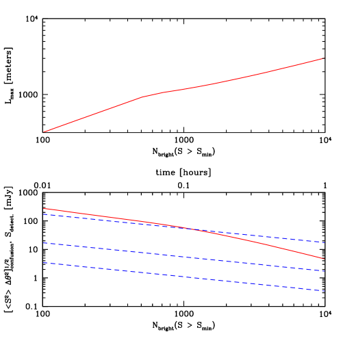
The resulting confusion noise, given an MWA pixel of angular size , is . In order to detect a point source of flux above the confusion noise from unresolved sources, we would like the flux from this source to be say times as large as the confusion noise, . This requirement demands high angular resolution: one needs relatively good angular resolution in order to beat down the confusion noise from the unresolved sources.
We investigate the angular resolution required to overcome confusion noise from unresolved point sources in Figure 6. First, we determine the minimum flux, , above which the MWA can detect point sources in its entire field of view. We then solve for the angular resolution such that the confusion noise from point sources with is less than – i.e., we require that the source is detectable above the confusion noise at significance. The angular resolution satisfying this constraint, , corresponds to a baseline with length . The figure illustrates that, in order to detect a few hundred point sources above the confusion noise – roughly the number of bright point sources required for MWA array calibration – one requires baselines of order km. Hence at least some antennae are required beyond the super-core configuration, which provides a maximum baseline of only m.
In order to determine how many antennae are needed at long baselines, we want to demand that the thermal detector noise of the large baseline antennae is much less than the source flux, , that we aim to detect. Let us take antennae at long baselines. The detector noise for point source detection, with antennae, each of effective area , integrating for hours over a bandwidth is:
| (5) |
We plot the thermal noise in the bottom panel of Figure 6 for a bandwidth of MHz, and m2 (appropriate for the MWA at ; Bowman et al. (2006)), as a function of for several different values of . On timescales of tens of seconds, the thermal noise expected for antennae at long baselines is much less than both the confusion noise and the minimum source flux required to detect a few hundred bright sources. This suggests that while some antennae are required at large baselines, the requirements are rather modest. In particular, only long baseline antennae are required by our simple estimate, leaving antennae for our super-core configuration. This is conservative, since we have effectively treated the antennas in the core as a single antenna in considering the calibration requirements. Our proposed arrangement is in marked contrast to the suggested distribution, in which only antennae are in a compact core.
From our simple estimates, it appears that the super-core, or a similar configuration, is feasible since only a handful of long baselines appear necessary for array calibration. This should, of course, be tested with detailed simulations of the MWA pipeline, performed for a variety of antenna distributions. While we have argued that the super-core is optimal for spherically-averaged 21 cm power spectrum estimates, it may not be optimal for other programs. Heliospheric science, and surveys for radio transients for example, will naturally require high angular resolution and favor less compact antenna configurations. Other EoR science projects may be impacted as well. For example, a compact-core is not ideal for detecting the 21 cm-galaxy cross power spectrum: here one needs to balance the MWA’s high sensitivity along the line of sight, but poor transverse sensitivity, with the galaxy survey’s poor line of sight sensitivity – owing to uncertainties in photometric redshifts – yet superior transverse sensitivity (Furlanetto & Lidz 2007). The MWA program to image quasar HII regions (Geil & Wyithe 2007) may also suffer from reduced angular resolution. In practice, the MWA might start with an configuration, or a slightly more compact arrangement, and gradually add antennae into a compact core.
4. Constraining the Power Spectrum Amplitude and Slope
Figure 3 suggests that the MWA will mainly be sensitive to the amplitude and the slope of the 21 cm power spectrum at each of several redshifts. Constraints on just these two numbers, in several redshift bins, are still quite interesting: we showed in §2.3 that the 21 cm power spectrum amplitude and slope evolve with redshift in a relatively generic and informative manner. Let us consider how well we can determine the parameters of a power law fit to the MWA power spectrum measurements in several redshift bins.
In practice, the MWA will be limited by large data rates to handling MHz intervals of bandwidth at a time. This MHz interval can be sampled in any manner desired from the full spectral range covered by the instrument, MHz – e.g., one could take MHz centered around and MHz around , or one could take a contiguous MHz stretch, etc. One can further sub-divide this MHz into smaller intervals for foreground-cleaning and power spectrum analyses. The best choice of frequencies to analyze depends, of course, on when reionization occurs.
For illustrative purposes, let us start with a contiguous MHz bin centered fortuitously on , when reionization is roughly complete in our model. We discuss less fortunate choices subsequently. We divide this up into five MHz redshift bins in which we separately estimate power spectrum errors, and discard the remaining MHz in our analysis. We consider observing this MHz stretch for a year, assuming, as above, that this yields hours of usable data. This stretch of MHz corresponds to a redshift range of .
In addition, we consider observations of a further contiguous stretch of MHz, expanding our redshift coverage out to . Again, we assume that this higher redshift stretch is observed for hours. The high redshift stretch might be observed roughly simultaneously with the lower redshift band – e.g., one day observing at low redshift followed by a day at high redshift – or one might observe consecutively for a year at low redshift, followed by a year at high redshift, etc. Either way, in total our estimates amount, optimistically, to two years of observing.
We then estimate error bars for the observing strategy described above, using the formulas in §3 for each of the redshift bins considered here. Further, we fit a polynomial function to in , truncating the fit at the lowest order that yields an unbiased estimate of the amplitude and slope of the power spectrum at the pivot wavenumber, :
| (6) |
Since the 21 cm power spectrum is not a perfect power law on MWA scales (Figure 1), it is important that we leave our fit reasonably general. We would like to ensure that our estimates of the amplitude and slope of the 21 cm power spectrum are unbiased: do the best fit amplitude and slope change by more than the error bars as we include more parameters in our fit? Further, we want to check whether the MWA is able to detect additional parameters in the generalized polynomial fit – e.g., a ‘running’ in the power law slope. We estimate the parameters , , and their errors assuming Gaussian statistics, and using standard maximum likelihood estimates. We fit to the simulation data given our power spectrum error estimates. We use all scales smaller than prohibited by foreground contamination, and restrict ourselves to Mpc-1, since smaller scales are too noisy to yield useful information.
We adopt Mpc-1 as the pivot wavenumber for our fit (Equation 6). This wavenumber is close to the middle of the range of scales probed, and represents a convenient choice. Note, however, that the sensitivity is a strong function of wavenumber and the power spectrum is constrained more tightly by the data on large scales than on small scales (Figure 3). This implies that estimates of the power spectrum amplitude and slope are correlated for our choice of , in contrast to the traditional choice of pivot scale in which amplitude and slope errors are uncorrelated. Provided we account for correlations in the amplitude and slope estimates, our final constraints on the ionization fraction (§5) are, however, independent of . The wave number at which the slope and amplitude errors are uncorrelated will depend on the foreground cut wavenumber, and on redshift. We hence prefer to plot results in the middle of the range of scales probed by the MWA, where the amplitude is a particularly strong function of ionization fraction, keeping in mind the error correlations. Moreover, note that the total for 21 cm power spectrum detection is larger than the significance at which the MWA can estimate the power spectrum amplitude at this particular scale (see §3.2), owing to the strong scale dependence of thermal noise.
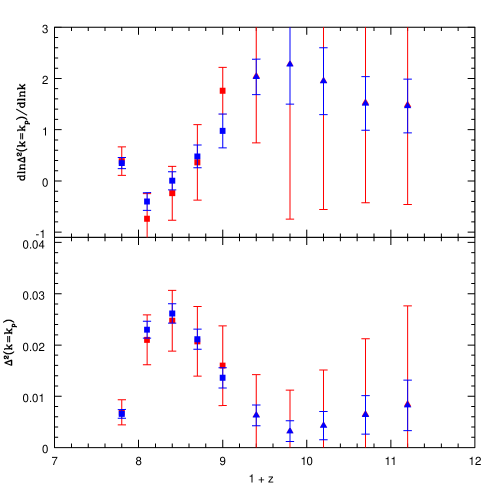
The results of our calculation are shown in Figure 7, for each of an antenna distribution, and the super-core configuration. In each redshift bin, as we detail shortly, we choose the minimum number of parameters in our fit (Equation 6) that yields an unbiased estimate of the 21 cm power spectrum amplitude and slope. Considering first the antenna distribution, the bottom panel of the figure shows that the MWA, in this configuration, can only weakly detect evolution in the power spectrum amplitude at Mpc-1 in our fiducial model. Still more marginal is the ability of the MWA, in the arrangement, to detect redshift evolution in the slope of the 21 cm power spectrum (top panel): one can almost draw a straight line through all of the error bars in this figure. The MWA, in the super-core configuration, however, enables significant detections of redshift evolution in both the slope and amplitude of the 21 cm power spectrum. As remarked previously, the slope and amplitude errors are significantly correlated. For example, the correlation coefficient between our amplitude and slope estimates is at in the super-core configuration, and at the same redshift for the antenna configuration.
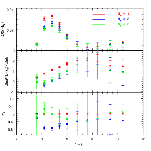
Before more closely considering the insights that can be gleaned from detecting this redshift evolution, let us briefly return to the question of the number of parameters required. We fit our model power spectra with plausible MWA error-bars in the super-core configuration, using a polynomial fit with each of , and . Similar considerations apply for the antenna distribution. The results of these fits are shown in Figure 8: the red squares show fits with included, the blue squares show fits with , and the green squares show fits with . The top panel shows constraints on power spectrum amplitude, the middle panel shows constraints on the slope, and the bottom panel shows constraints on the ‘running’ of the slope, .
We judge our estimate of a parameter ‘unbiased’ if the preferred value of that parameter changes by less than when an additional parameter is included in the fit. For example, our estimate of the power spectrum amplitude near changes by more than one sigma when we move from to , and we consider it biased. Likewise, estimates of the slope of the 21 cm power spectrum are biased in several redshift bins for . For the slope and the amplitude, estimates converge in all redshift bins by . In each redshift bin we include the minimum number of parameters required to provide an unbiased estimate of the amplitude and slope, so we include only parameters up to in some redshift bins, while we include parameters up to in others. In some of our most tightly constrained redshift bins there initially appears to be a constraint on . Including an additional parameter in the fit, , shows that our constraint on is biased for . Hence, while we include as a parameter in some redshift bins, we only use our constraints on the amplitude and slope, since only these parameters are unbiased.
Provided the MWA packs enough antennae into its core, it does have the sensitivity to detect redshift evolution in the slope and amplitude of the 21 cm power spectrum, if not higher terms in the polynomial fit of Equation (6). While our forecasts are inevitably idealized, the constraints are tight enough that we expect a reasonable detection of redshift evolution for our fiducial model in the super-core configuration.
Of course, reionization may be more extended and/or occur at higher redshift than in our fiducial model. The calculations of §3 give some insight into the impact of the timing of reionization on MWA detection sensitivity. For example, Figure 4 implies that we still expect a significant detection of 21 cm fluctuations if reionization is already complete at the highest redshift probed by our hypothetical MWA survey. In this scenario, however, the MWA would observe only the falling half of our anticipated trend of 21 cm power spectrum amplitude with redshift, and miss the earlier phase in which we expect the 21 cm power spectrum amplitude to grow with decreasing redshift. Moreover, reionization may be more extended than in our fiducial model and lead to a more gradual power spectrum maximum when fluctuations are measured as a function of redshift.
5. The Filling Factor of HII Regions from Power Spectrum Measurements
Let us turn our error estimates on the 21 cm power spectrum amplitude and slope into constraints on the filling factor of HII regions during reionization. As an illustration, we focus on power spectrum measurements in the specific redshift bin where the amplitude is maximal – i.e., our input ‘true’ model is our fiducial model with . We compare our simulated signal in this redshift bin, including MWA statistical error estimates, with fiducial model predictions at different ionization fractions. We compute between the different models, and calculate the likelihood that the data are drawn from a fiducial model with a given ionization fraction, assuming Gaussian statistics, . We assume in these calculations that our model 21 cm power spectra are entirely fixed by and ignore the weak redshift dependence expected. Since our estimates of the amplitude and slope are correlated, we use the full co-variance matrix to compute .
We assume our fiducial model to calculate power spectra at different ionization fractions, ignoring model uncertainties in 21 cm power spectra at a given ionization fraction. This is justified – at least for the model of ionization fraction evolution we assume here – since the MWA can rule out the rare-source and mini-halo models by comparing measurements over the full redshift range. Specifically, we translate the power spectrum amplitude and slope measurements of Figure 7 from measurements as a function of redshift to measurements as a function of ionization fraction, assuming our fiducial model to convert between redshift and ionization fraction. We then compare our mock 21 cm power spectrum amplitude and slope measurements with the rare source and mini-halo models, computing between these models and our fiducial model. We find that the MWA can distinguish between these models at very high significance – both the mini-halo and rare source model are ruled out at confidence even with the antenna configuration.666In detail, we should marginalize over the uncertain relation – which is what we ultimately aim to constrain – when constraining the rare source and mini-halo models. For simplicity, we assume the fiducial relation in comparing with the rare source and mini-halo models, and find that these models are very strongly ruled out. From Figure 2, we believe these constraints are strong enough that they would not be alleviated by marginalizing over . This means that the MWA can break degeneracies between the different models, and we can get approximate error estimates on the ionization fraction from our fiducial model alone.

The results of our ionization fraction likelihood calculations are shown in Figure 9. The MWA, observing in the configuration, will provide a modest constraint on the ionization fraction at maximal amplitude: ionization fractions between are allowed at confidence. The constraint is only modest because the slope and amplitude measurements have rather large error bars in this configuration (Figure 9), and because the amplitude and slope are fairly flat functions of ionization fraction around the peak (Figure 2). The constraint is tighter at low ionization fraction than one might naively guess from eye-balling the results of Figure 2, however, since the slope and amplitude errors are correlated. In particular, data drawn from our low ionization fraction models will tend to have a smaller amplitude, yet a steeper slope, than data drawn from our model. Properly accounting for correlations between our slope and amplitude estimates then increases the constraint on low ionization fraction models, compared to ignoring these correlations.
On the other hand, the MWA observing in the super-core configuration provides a bit tighter constraint. Only is allowed at confidence. Comparing the blue solid and dashed curves in the figure illustrates that most of the constraint comes from the amplitude measurement and not the slope measurement. Provided the middle phase of reionization occurs in the MWA observing band, a couple of years of observations should constrain around to within roughly at confidence.
6. Conclusions
In this paper, we considered the sensitivity of the MWA for 21 cm power spectrum measurements and examined the resulting insights into reionization. Rather generically, the 21 cm power spectrum on MWA scales increases in amplitude with decreasing redshift, as HII regions grow and boost the level of large-scale fluctuations in the 21 cm signal, until the time at which of the volume of the IGM is ionized. Subsequently, later in the EoR, the amplitude of the 21 cm power spectrum drops as neutral hydrogen becomes scarce. In conjunction, the slope of the 21 cm power spectrum flattens as HII regions grow and the 21 cm power spectrum transitions, on the scales of interest, from simply tracing density fluctuations to tracing fluctuations in the ionization field.
These generic features imply that, although MWA measurements will be limited to a dynamic range of a decade in scale, the experiment can significantly constrain reionization by comparing measurements in several redshift bins. In particular, the MWA may detect the power spectrum amplitude rise with decreasing redshift, before subsequently turning-over and dropping in amplitude, with the slope of the power spectrum flattening in conjunction. This behavior is a signature of the IGM passing through a redshift where of its volume is filled with ionized bubbles.
It is unlikely that residual foreground contamination would share the characteristic redshift evolution in power spectrum amplitude and slope found in our models. Measuring this characteristic redshift evolution will hence help confirm that detected 21 cm fluctuations originate from the high redshift IGM, and cement the case for neutral material in the high redshift IGM.
We argued that the MWA is sensitive enough to detect this characteristic redshift evolution in the 21 cm power spectrum amplitude and slope, especially if it adopts a very compact configuration for its antenna tiles, and that reionization occurs at sufficiently moderate redshifts. A compact configuration optimizes power spectrum sensitivity because proposed configurations, with antennae distributed out to large km distances, populate long baselines too sparsely to be useful. Some antenna tiles are needed at long baselines for point source detection and antenna calibration, but we estimate that these requirements are not severe.
Another possible advantage of the super-core configuration relates to its well-behaved beam. A potential difficulty for 21 cm observations is that point sources far from the primary beam of an interferometer can enter through the beam’s sidelobes, which are frequency dependent. This contamination will have structure in frequency space, and escape the usual foreground removal strategies (e.g. Oh & Mack 2003, Furlanetto et al. 2006a). This contamination will be significantly reduced by adopting a very compact antenna distribution, like the super-core configuration, which will have a very clean beam with minimal sidelobes.
Adopting a sufficiently compact antenna distribution, we believe that the MWA can move past a mere detection of 21 cm fluctuations, and constrain the volume filling factor of HII regions within two years of observing. In particular, measurements of the 21 cm power spectrum amplitude and slope at a redshift where of the volume is ionized translate into allowed ionization fractions of roughly . Moreover, we find that the MWA can rather easily distinguish between our fiducial model and each of our rare source and mini-halo models with hours of data, at least if the bulk of reionization occurs in the range of redshifts probed by the MWA.
In this paper, we focused on the 21 cm power spectrum, but investigating other statistical measures would be interesting. One of the primary goals of reionization studies is to use observational measures to constrain the sizes and filling factor of HII regions during reionization. Clearly the ionization field, and the 21 cm signal, are highly non-Gaussian in the EoR, implying that there is, in principle, more information than contained in the 21 cm power spectrum alone. We have argued that the redshift evolution of the 21 cm power spectrum contains relatively robust information regarding the filling factor of HII regions during reionization, but these constraints may not be optimal and are rather indirect. On the other hand, it is unclear how beneficial higher order statistics will be in the low regime relevant for the MWA and other first generation surveys. We plan further investigation regarding the utility of various non-Gaussian statistical measures, considered as a function of instrumental sensitivity. Particularly interesting is that some low- bins become sample-variance dominated in the super-core configuration, implying that the MWA can actually image large scale modes in this configuration.
Another useful endeavor would be to perform a mock MWA simulation, incorporating thermal noise, foreground models, and the MWA instrumental response and observing strategy. Our forecasts are inevitably simplified in ignoring these details, and likely optimistic in this regard. Mock simulations should quantify how much the sensitivity of the MWA is degraded when incorporating such real world details. Moreover, it would be interesting to examine how possible residuals from incomplete foreground cleaning might bias our constraints. Since the power spectrum variance increases strongly with wavenumber, the total at which the MWA can detect the 21 cm power spectrum depends strongly on the precise foreground cut. This is an important issue for further investigation.
Finally, in this paper we focused on a single parameter, the filling factor of ionized regions at different redshifts, and gave simple arguments for how one can constrain this quantity with the redshift evolution of the 21 cm power spectrum alone. A complementary approach for forecasting MWA parameter constraints would be to perform a multi-parameter Fisher matrix analysis.
We anticipate that the MWA will swiftly move beyond a mere detection of 21 cm emission from the high redshift IGM, and obtain valuable insights regarding the filling factor of HII regions at different stages of reionization.
Acknowledgments
We are grateful to Suvendra Dutta for help with the simulations used in this analysis, and for useful discussions. We thank Miguel Morales for comments on a draft, and for informative discussions, and Judd Bowman and Peng Oh for helpful conversations. The authors are supported by the David and Lucile Packard Foundation, the Alfred P. Sloan Foundation, and grants AST-0506556 and NNG05GJ40G. OZ thanks the Berkeley Center for Cosmological Physics for support.
References
- (1) Abel, T., & Wandelt, B. D. 2002, MNRAS, 330, 53
- (2) Barkana, R., & Loeb, A. 2001, Phys. Rept., 349, 125
- (3) Becker, G. D., Rauch, M., & Sargent, W. L. W. 2007, ApJ, 662, 72
- (4) Bolton, J. S., & Haehnelt, M. G. 2007a, MNRAS, 374, 493
- (5) Bolton, J. S., & Haehnelt, M. G. 2007b, MNRAS, 381L, 35
- (6) Bowman, J. D., Morales, M. F., & Hewitt, J. N. 2006, ApJ, 638, 20
- (7) Croft, R. A. C., & Altay, G. 2007, ApJ submitted, arXiv:0709.2362
- (8) Dijkstra, M., Wyithe, J. S. B., & Haiman, Z. 2007, MNRAS, 379, 253
- (9) Di Matteo, T., Perna, R., Abel, T., & Rees, M. J. 2002, ApJ, 564, 576
- (10) Fan, X. et al. 2006, AJ, 132, 117
- (11) Furlanetto, S. R., Zaldarriaga, M., & Hernquist, L. 2004, ApJ, 613, 1
- (12) Furlanetto, S. R., & Oh, S. P., 2005, MNRAS, 363, 1031
- (13) Furlanetto, S. R., Oh, S. P., & Briggs, F. 2006a, Phys. Reports, 433, 181
- (14) Furlanetto, S. R., McQuinn, M., & Hernquist, L. 2006b, MNRAS, 365, 115
- (15) Furlanetto, S. R., Zaldarriaga, M., & Hernquist, L. 2006c, MNRAS, 365, 1012
- (16) Furlanetto, S. R., & Lidz, A. 2007, ApJ, 660, 1030
- (17) Gallerani, S., Ferrara, A., Fan, Z., & Choudhury, T. R. 2007, MNRAS submitted, astro-ph/0706.1053
- (18) Geil, P. M., & Wyithe, J. S. B. 2007, MNRAS submitted, astro-ph/0708.3716
- (19) Gnedin, N. Y., & Shaver, P. A. 2004, ApJ, 608, 611
- (20) Hales, S. E. G., Baldwin, J. E., & Warner, P. J. 1988, MNRAS, 234, 919
- (21) Iliev, I. T., Shapiro, P. R., & Raga, A. C. 2005, MNRAS, 361, 405
- (22) Iliev, I. T., Mellema, G., Pen, U. L., Merz, M., Shapiro, P. R., & Alvarez, M. A. 2006, MNRAS, 369, 1625
- (23) Kashikawa, N., et al. 2006, ApJ, 648, 7
- (24) Kohler, K., Gnedin, N. Y., & Hamilton, A. J. S. 2005, ApJ submitted, astro-ph/0511627
- (25) Lidz, A., Oh, S. P., & Furlanetto, S. R. 2006, ApJL, 639, 47
- (26) Lidz, A., McQuinn, M., Zaldarriaga, Hernquist, L., & Dutta, S., 2007a, ApJ in press, astro-ph/0703667
- (27) Lidz, A., Zahn, O., McQuinn, M., Zaldarriaga, M., Dutta, S., & Hernquist, L. 2007b, ApJ, 659, 865
- (28) Madau, P., Meiksin, A., & Rees, M. J. 1997, ApJ, 475, 429
- (29) Malhotra, S., & Rhoads, J. 2005, ApJL submitted, astro-ph/0511196
- (30) McQuinn, M., Zahn, O., Zaldarriaga, M., Hernquist, L., & Furlanetto, S. R. 2006, ApJ, 653, 815
- (31) McQuinn, M., Lidz, A., Zahn, O., Dutta, S., Hernquist, L., & Zaldarriaga, M. 2007a, MNRAS, 377, 1043
- (32) McQuinn, M., Hernquist, L., Zaldarriaga, M., & Dutta, S., 2007b, MNRAS in press, astro-ph/0704.2239
- (33) McQuinn, M., Lidz, A., Zaldarriaga, M., Hernquist, L., & Dutta, S., 2007c, MNRAS submitted, arXiv:0710.1018
- (34) Mesinger, A., & Haiman, Z. 2007, ApJ, 660, 923
- (35) Mesinger, A., & Furlanetto, S. R. 2007a, MNRAS submitted, astro-ph/0708.0006
- (36) Mesinger, A., & Furlanetto, S. R. 2007b, ApJ submitted, astro-ph/0704.0946
- (37) Morales, M. F., & Hewitt, J. 2004, ApJ, 615, 7
- (38) Morales, M. F. 2005, ApJ, 619, 678
- (39) Morales, M. F., Bowman, J. D., & Hewitt, J. N. 2006, ApJ, 648, 767
- (40) Oh, S. P., & Haiman, Z. 2003, MNRAS, 346, 456
- (41) Oh, S. P., & Mack, K. J. 2003, MNRAS, 346, 871
- (42) Page, L. et al. 2007, ApJS, 170, 335
- (43) Pritchard, J. R., & Furlanetto, S. R. 2007, MNRAS, 376, 1680
- (44) Shapiro, P. R., Iliev, I. T., & Raga, A. C. 2004, MNRAS, 348, 753
- (45) Sokasian, A., Abel, T., & Hernquist, L. 2001, NewA, 6, 359
- (46) Sokasian, A., Abel, T., Hernquist, L. & Springel, V. 2003, MNRAS, 344, 607
- (47) Spergel, D. N., et al., 2007, ApJS, 170, 377
- (48) Springel, V. 2005, MNRAS, 364, 1105
- (49) Totani, T. et al. 2006, PASJ, 58, 485
- (50) Trac, H., & Cen, R., 2006, ApJ in press, astro-ph/0612406
- (51) Wyithe, J. S. B., Loeb, A., & Carilli, C., 2005, ApJ, 628, 575
- (52) Wyithe, J. S. B., Bolton, J., & Haehnelt, M. 2007, MNRAS submitted, arXiv:0708.1788
- (53) Wyithe, J. S. B., & Loeb, A. 2007, MNRAS submitted, arXiv:0708.3392
- (54) Wyithe, J. S. B., & Morales, M. 2007, MNRAS submitted, astro-ph/0703070
- (55) Zahn, O., Lidz, A., McQuinn, M., Dutta, S., Hernquist, L., Zaldarriaga, M., & Furlanetto, S. R. 2007, ApJ, 654, 12
- (56) Zaldarriaga, M., Furlanetto, S. R., & Hernquist, L. 2004, ApJ, 608, 622