Generation of Large-Scale Magnetic Fields in Single-Field Inflation

Abstract

We consider the generation of large-scale magnetic fields in slow-roll inflation. The inflaton field is described in a supergravity framework where the conformal invariance of the electromagnetic field is generically and naturally broken. For each class of inflationary scenarios, we determine the functional dependence of the gauge coupling that is consistent with the observations on the magnetic field strength at various astrophysical scales and, at the same time, avoid a back-reaction problem. Then, we study whether the required coupling functions can naturally emerge in well-motivated, possibly string-inspired, models. We argue that this is non trivial and can be realized only for a restricted class of scenarios. This includes power-law inflation where the inflaton field is interpreted as a modulus. However, this scenario seems to be consistent only if the energy scale of inflation is low and the reheating stage prolonged. Another reasonable possibility appears to be small field models since no back-reaction problem is present in this case but, unfortunately, the corresponding scenario cannot be justified in a stringy framework. Finally, large field models do not lead to sensible model building.

1 Introduction

Magnetic fields are present on various scales in the Universe from planets, stars, galaxies, to clusters of galaxies, see e.g., Refs. [1, 2, 3] for reviews. In galaxies of all types, magnetic fields with the field strength $\sim 10^{-6}$ G, ordered on $1-10$ kpc scale, have been detected [3, 4]. There is also some evidence that they exist in galaxies at cosmological distances [5]. Furthermore, in recent years, magnetic fields in clusters of galaxies have been observed by means of the Faraday rotation measurements (RMs) of polarized electromagnetic radiation passing through an ionized medium [6, 7, 8]. Unfortunately, however, RMs give only the product of the field strength along the line of sight and the coherence scale, and we cannot find them independently. In this situation, the strength and the scale are estimated on $10^{-7}-10^{-6}$ G and 10 kpc$-$1 Mpc, respectively. It is interesting that magnetic fields in clusters of galaxies are as strong as galactic ones and that the coherence scale may be as large as $\sim$ Mpc.

Since the conductivity of the Universe through most of its history is large, the magnetic field $B$ evolves conserving magnetic flux as $B\propto a^{-2}$, where $a(t)$ is the scale factor. On the other hand, the average cosmic energy density $\bar{\rho}$ evolves as $\bar{\rho}\propto a^{-3}$. Hence, the scaling of the magnetic field is given by $B\propto{\bar{\rho}}^{2/3}$ and this relation should also be understood as giving the value of $B$ at different spatial locations characterized by different energy densities. The present ratio of interstellar medium density in galaxies ${\rho}_{\mathrm{gal}}$ to $\bar{\rho}$ and that of inter-cluster medium density in clusters of galaxies ${\rho}_{\mathrm{cl}}$ are ${\rho}_{\mathrm{gal}}/\bar{\rho}\simeq 10^{5}-10^{6}$ and ${\rho}_{\mathrm{cl}}/\bar{\rho}\simeq 10^{2}-10^{3}$, respectively. Consequently, from these relations, we see that, using the law mentioned before, namely $\bar{B}=B_{\mathrm{gal,cl}}(\rho_{\mathrm{gal,cl}}/\bar{\rho})^{-2/3}$, the required strength of the cosmic magnetic field at the structure formation, adiabatically rescaled to the present time, is $10^{-10}-10^{-9}\mathrm{G}$ in order to explain the observed fields mentioned before. On the other hand, in general, if the galactic dynamo mechanism is at play, then seed fields with a present strength of only $10^{-22}-10^{-16}\mathrm{G}$ is required [9, 10, 11].

The question addressed in this article is that of the origin of these magnetic fields and whether there exists simple, physically well-motivated mechanisms, which could provide the target values of $B$ just described above. Generation mechanisms of the seed magnetic fields fall into two broad categories. One is astrophysical processes and the other is cosmological physical processes in the early Universe. The former exploits the difference in mobility between electrons and ions. This difference can lead to electric currents and hence magnetic fields. If the scale of cluster magnetic fields is as large as $\sim$ Mpc, however, it is unlikely that the origin of such a large-scale magnetic field is in astrophysical processes and we are tempted to assign the origin of cosmological magnetic field to the processes during inflation in the early Universe which stretches coherent scales exponentially [12, 13, 14, 15, 16, 17, 18, 19, 20].

During inflation quantum scalar (density) perturbations [21, 22, 23, 24] and tensor (gravitational waves) perturbations [25, 26] are generated and stretched to cosmological scales by subsequent accelerated expansion. Usually, however, large scale fluctuations in electromagnetic fields are not generated, because they are conformally invariant [27]. Hence, in order to generate cosmological magnetic fields during inflation, one must break the conformal invariance of the theory in an appropriate manner. A number of models have been proposed in this context so far [28, 29, 30, 31, 32, 33, 34, 35, 36, 37, 38, 39, 40].

Here we propose a simple model making use of the arbitrariness of the gauge kinetic function in supergravity [41]. Indeed, the general supergravity Lagrangian including vector super-multiplets contains the following term

$$\int{\rm d}^{2}\theta\left[f_{ab}(\Phi)W_{a}{}^{\alpha}W_{\alpha b}+\mbox{h.c.}\right]\,,$$ (1)

where $W_{a}{}^{\alpha}$ is the gauge field strength superfield with spinor index $\alpha$ and gauge group index $a$. As already mentioned, the quantity $f_{ab}(\Phi)$ is an arbitrary function of the chiral superfield $\Phi$ [42]. This implies that the conformal invariance is naturally and generically broken as is most conveniently shown when the above term is expressed in terms of the superfields components

$$\frac{1}{4}\Re f_{ab}(\phi)\left(F_{a}\right)_{\mu\nu}\left(F_{b}\right)^{\mu\nu}\,.$$ (2)

Since we are interested in the production of magnetic fields, we consider a $U(1)$ gauge field and, therefore, the gauge field strength do no longer carry a gauge index. As a consequence, there is also only one function $f(\phi)$ left. Moreover, in order to consider the minimalist case with the least possible assumptions, we naturally identify the scalar part $\phi$ of the chiral superfield $\Phi$ to the inflaton field.

A related study was carried out in Refs. [29, 30] but only in the particular case where $f(\phi)\propto{\rm e}^{\phi}$. Here, we study the most general case (at least, in the framework of single field inflation) and determine which form $f(\phi)$ should take in order to obtain a power spectrum of the magnetic field in agreement with the currently available observational constraints on large scales. Then, for each category of single field inflationary scenarios, we explore whether there is a natural model in supergravity (possibly string-inspired) that could reproduce the required shape of the gauge coupling and, at the same time, leads to the correct form of the inflaton potential.

This paper is organized as follows. In Sec. 2, we describe our model action and derive the equations of motion from it. Then, the gauge field is quantized in the Coulomb gauge and the vacuum energy density of the magnetic field at the end of inflation is determined. The evolution of the magnetic energy density through the subsequent stages of evolution, preheating, radiation and matter dominated eras is also computed. In a next step, for each single field slow-roll inflationary models, using a simple ansatz depending only on one free parameter, we calculate the required shape of the gauge coupling function $f(\phi)$. In Sec. 3, we use the currently available limits on the magnetic field to constraint the free parameter mentioned above, that is to say to constraint the shape of the gauge coupling function. We also investigate the consistency of the model and determine under which conditions this one does not suffer from a back-reaction problem. In Sec. 4, we try to embed in particle physics the models that have been shown to be phenomenologically viable. Finally, in Sec. 5, we present our conclusions. Throughout this article, we use units in which $c=\hbar=M_{G}=k_{\mathrm{B}}=1$. We also put the reduced Planck mass, $M_{G}\equiv 1/\sqrt{8\pi G}$, to unity when it simplifies the notation. In this case, the full Planck scale takes $m_{\scriptscriptstyle{\mathrm{Pl}}}\equiv G^{-1/2}=\sqrt{8\pi}$.

2 Reverse-Engineering of the Magnetic Field

2.1 Magnetic Field during Inflation

During inflation, following the considerations presented in Sec. 1, the action of the system, namely a scalar inflaton field plus a $U(1)$ gauge field, can be written as

$$S\left[\phi,A_{\mu}\right] = -\int{\rm d}^{4}x\sqrt{-g}\left[\frac{1}{2}g^{\mu\nu}\partial_{\mu}\phi\partial_{\nu}\phi+V(\phi)\right]$$ (3)

$$-\frac{1}{4}\int{\rm d}^{4}x\sqrt{-g}g^{\alpha\beta}g^{\mu\nu}f^{2}\left(\phi\right)F_{\mu\alpha}F_{\nu\beta}\,,$$

with $F_{\mu\alpha}\equiv\partial_{\mu}A_{\alpha}-\partial_{\alpha}A_{\mu}$, $A_{\alpha}$ being the vector potential whose dimension is that of a mass $[A_{\mu}]=M$. The inflaton potential $V(\phi)$ and the dimensionless gauge coupling $f(\phi)$ are, a priori, arbitrary functions. Notice that we have changed the definition of the gauge coupling (now $f^{2}$ appears in the action rather than $f$) for future convenience. The equations of motion following from the above action can be written as

$$\frac{1}{\sqrt{-g}}{\partial}_{\mu}\left(\sqrt{-g}g^{\mu\nu}{\partial}_{\nu}\phi\right)-\frac{{\rm d}V}{{\rm d}\phi} = \frac{1}{4}\frac{{\rm d}f(\phi)}{{\rm d}\phi}F_{\mu\nu}F^{\mu\nu}\,,$$ (4)

$$\partial_{\mu}\left[\sqrt{-g}g^{\mu\nu}g^{\alpha\beta}f^{2}\left(\phi\right)F_{\nu\beta}\right] = 0\,.$$ (5)

In the following, we consider that the electromagnetic field is a perturbatively small quantity (a “test” field) compared with the inflaton counterpart. This means that one can neglect the right hand side of the Klein-Gordon equation and work in a spatially flat Friedmann-Lemaître-Robertson-Walker (FLRW) space-time,

$${\rm d}s^{2}=g_{\mu\nu}{\rm d}x^{\mu}{\rm d}x^{\nu}=-{\rm d}t^{2}+a^{2}(t){\rm d}{{\mbox{\boldmath$x$\unboldmath}}}^{2}=a^{2}(\eta)\left(-{\rm d}\eta^{2}+{\rm d}{{\mbox{\boldmath$x$\unboldmath}}}^{2}\right)\,,$$ (6)

where $t$ is the cosmic time and $\eta$ the conformal one, since the gauge field being negligible there is no preferred direction. Therefore, the equations of motion are just the standard ones, namely

$$H^{2} = \left(\frac{\dot{a}}{a}\right)^{2}=\frac{1}{3}\left[\frac{1}{2}{\dot{\phi}}^{2}+V(\phi)\right]\,,\quad\frac{1}{a^{2}}{\cal H}^{2}=\frac{1}{3}\left[\frac{1}{2a^{2}}{\phi^{\prime}}^{2}+V(\phi)\right]\,,$$ (7)

with ${\cal H}\equiv a^{\prime}/a$ and, for the inflaton field,

$$\ddot{\phi}+3H\dot{\phi}+\frac{{\rm d}V}{{\rm d}\phi}=0\,,\quad\phi^{\prime\prime}+2{\cal H}\phi^{\prime}+\frac{{\rm d}V}{{\rm d}\phi}=0\,.$$ (8)

In order to simplify the calculations, we adopt the Coulomb gauge where $A_{0}(t,{\mbox{\boldmath$x$\unboldmath}})=0$ and ${\partial}_{j}A^{j}(t,{\mbox{\boldmath$x$\unboldmath}})=0$. In this case, one obtains

$$\ddot{A_{i}}(t,{\mbox{\boldmath$x$\unboldmath}})+\left(H+2\frac{\dot{f}}{f}\right)\dot{A_{i}}(t,{\mbox{\boldmath$x$\unboldmath}})-{\partial}_{j}{\partial}^{j}A_{i}(t,{\mbox{\boldmath$x$\unboldmath}}) = 0\,,$$ (9)

$$A_{i}^{\prime\prime}+2\frac{f^{\prime}}{f}A_{i}^{\prime}-a^{2}\partial_{j}\partial^{j}A_{i} = 0\,,$$ (10)

where, of course, $\partial^{j}=g^{jk}\partial_{k}=(\delta^{jk}/a^{2})\partial_{k}$. If one defines $\bar{A}_{j}\equiv fA_{j}$, then one can absorb the part proportional to the first derivative of the vector potential and put the equation of motion under the standard form of an equation for an oscillator. One gets

$$\bar{A}_{i}^{\prime\prime}-\frac{f^{\prime\prime}}{f}\bar{A}_{i}-a^{2}\partial_{j}\partial^{j}\bar{A}_{i}=0\,.$$ (11)

We see that, if $f=1$, the equation of motion of $A^{j}$ reduces to that of an harmonic oscillator. Due to the conformal coupling of the gauge sector, the dynamics is non trivial only if $f$ is not a constant.

Let us now (covariantly) define the electric and magnetic fields seen by an observer characterized by the four-velocity vector $u^{\mu}$. One has [43]

$$E_{\mu}=u^{\nu}F_{\mu\nu}\,,\quad B_{\mu}=\frac{1}{2}\epsilon_{\mu\nu\kappa}F^{\nu\kappa}\,,$$ (12)

where the tensor $\epsilon_{\mu\nu\kappa}$ is defined by the relation

$$\epsilon_{\mu\nu\kappa}=\eta_{\mu\nu\kappa\lambda}u^{\lambda}\,,$$ (13)

$\eta_{\mu\nu\kappa\lambda}$ being the totally antisymmetric permutation tensor of space-time with $\eta^{0123}=(-g)^{-1/2}$ or $\eta_{0123}=(-g)^{1/2}$. Therefore, for a comoving observer with $u^{\mu}=\left(1,{\mbox{\boldmath$0$\unboldmath}}\right)$ (in cosmic time), one gets

$$E_{i}=-\dot{A}_{i}\,,\quad B_{i}=\frac{1}{a}\epsilon_{ijk}\partial_{j}A_{k}\,,$$ (14)

with $\epsilon_{123}=1$. A remark is in order concerning the formula giving the magnetic field. Contrary to the previous expressions, it is not written in a covariant way and, therefore, the position of the indices is irrelevant even if implicit summation is still present. So, for instance, this formula simply means $B_{1}=(\partial_{2}A_{3}-\partial_{3}A_{2})/a$. As expected, the dimension of the magnetic field is two, $[B_{i}]=M^{2}$.

We now turn to the quantization of the system. It follows from Eq. (3) that the momentum conjugate to the gauge field $A_{i}(t,{\mbox{\boldmath$x$\unboldmath}})$ is given by

$$\pi^{i}(t,{\mbox{\boldmath$x$\unboldmath}})=\frac{\delta S}{\delta\dot{A}_{i}}=f^{2}(\phi)a^{3}(t)g^{ij}\dot{A_{j}}(t,{\mbox{\boldmath$x$\unboldmath}})=f^{2}(\phi)a^{2}(\eta)g^{ij}A_{j}^{\prime}(\eta,{\mbox{\boldmath$x$\unboldmath}})\,,$$ (15)

which also implies that $\pi_{i}(t,{\mbox{\boldmath$x$\unboldmath}})=f^{2}(\phi)a^{3}(t)\dot{A_{i}}(t,{\mbox{\boldmath$x$\unboldmath}})$. For quantization, we impose the canonical commutation relation between $A^{i}(t,{\mbox{\boldmath$x$\unboldmath}})$ and ${\pi}_{j}(t,{\mbox{\boldmath$x$\unboldmath}})$:

$$\left[A^{i}(t,{\mbox{\boldmath$x$\unboldmath}}),{\pi}_{j}(t,{\mbox{\boldmath$y$\unboldmath}})\right] = i\int\frac{{\rm d}^{3}{\mbox{\boldmath$k$\unboldmath}}}{{(2\pi)}^{3}}{\rm e}^{i{\mbox{\boldmath$\scriptstyle{k}$\unboldmath}}\cdot\left({\mbox{\boldmath$\scriptstyle{x}$\unboldmath}}-{\mbox{\boldmath$\scriptstyle{y}$\unboldmath}}\right)}\left({\delta}^{i}{}_{j}-\delta_{j\ell}\frac{k^{i}k^{\ell}}{k^{2}}\right)$$ (16)

$$= i\delta^{(3)}_{\perp}{}^{i}{}_{j}\left({\mbox{\boldmath$x$\unboldmath}}-{\mbox{\boldmath$y$\unboldmath}}\right)\,,$$ (17)

where $\delta^{(3)}_{\perp ij}$ is the transverse delta function introduced in order to have a consistent quantization in the Coulomb gauge.

In order to define the creation and annihilation operators, one has to Fourier expand the vector potential operator. For this purpose, one introduces an orthonormal basis in space-time defined by (in conformal time)

$$\epsilon_{0}^{\mu}=\left(\frac{1}{a},{\mbox{\boldmath$0$\unboldmath}}\right)\,,\quad\epsilon_{\lambda}^{\mu}=\left(0,\frac{\tilde{\epsilon}_{\lambda}^{i}}{a}\right)\,,\quad\epsilon_{3}^{\mu}=\left(0,\frac{1}{a}\frac{k^{i}}{k}\right)\,,$$ (18)

where $\lambda=1,2$ and where, by definition, $\delta_{ij}\tilde{\epsilon}_{\lambda}^{i}\tilde{\epsilon}_{\lambda}^{j}\equiv 1$ (no summation on $\lambda$). In the above equations, $k^{i}=ak^{i}_{\rm phys}$ is the comoving wavenumber satisfying $\delta_{ij}k^{i}k^{j}=k^{2}$. In addition, $\epsilon_{\lambda}^{\mu}\epsilon_{3\mu}=\tilde{\epsilon}_{\lambda}^{i}k_{i}=0$ which expresses the Coulomb gauge in Fourier space. Notice that, without the factor $1/a$ in the previous definitions, the above vectors would not be correctly normalized in curved space-time. Then, one has the covariant completeness relation $\sum_{s=0}^{s=3}g_{ss}\epsilon^{\mu}_{s}\epsilon^{\nu}_{s}=g^{\mu\nu}$ where $g_{ss}$ is just a factor which stands for $+1$ or $-1$. Projected on space, the completeness relation reduces to

$$\sum_{\lambda=1}^{2}\epsilon^{i}_{\lambda}({\mbox{\boldmath$k$\unboldmath}})\epsilon_{j\lambda}({\mbox{\boldmath$k$\unboldmath}})+\delta_{j\ell}\frac{k^{i}k^{\ell}}{k^{2}}=\delta^{i}{}_{j}\,.$$ (19)

Finally, the expression of $A_{i}(t,{\mbox{\boldmath$x$\unboldmath}})$ can be written as

$$A_{i}(\eta,{\mbox{\boldmath$x$\unboldmath}}) = \int\frac{{\rm d}^{3}k}{(2\pi)^{3/2}}\sum_{\lambda=1}^{2}\epsilon_{i\lambda}({\mbox{\boldmath$k$\unboldmath}})\biggl{[}b_{\lambda}({\mbox{\boldmath$k$\unboldmath}})A(\eta,k){\rm e}^{i{\mbox{\boldmath$\scriptstyle{k}$\unboldmath}}\cdot{\mbox{\boldmath$\scriptstyle{x}$\unboldmath}}}$$ (20)

$$+b_{\lambda}^{\dagger}({\mbox{\boldmath$k$\unboldmath}}){A}^{*}(\eta,k){\rm e}^{-i{\mbox{\boldmath$\scriptstyle{k}$\unboldmath}}\cdot{\mbox{\boldmath$\scriptstyle{x}$\unboldmath}}}\biggr{]},$$

in terms of the annihilation and creation operators, $b_{\lambda}({\mbox{\boldmath$k$\unboldmath}})$ and $b_{\lambda}^{\dagger}({\mbox{\boldmath$k$\unboldmath}})$, with $k$ being the comoving wavenumber. The quantity $\epsilon_{i}^{\lambda}({\mbox{\boldmath$k$\unboldmath}})$ is the transverse polarization vector and has been defined before and the time-dependent Fourier amplitude obeys the following equation of motion

$${\cal A}^{\prime\prime}(\eta,k)+\left(k^{2}-\frac{f^{\prime\prime}}{f}\right){\cal A}(\eta,k)=0$$ (21)

where ${\cal A}(\eta,k)\equiv a(\eta)f(\eta)A(\eta,k)$. The additional factor $a$ in the previous definition originates from the presence of the vector $\epsilon_{i\lambda}({\mbox{\boldmath$k$\unboldmath}})$ in the Fourier expansion (20) of the gauge field. The dimension of the Fourier amplitude of the gauge field is $[A]=M^{-1/2}$ since $[A_{i}]=M$ and $[b_{\lambda}({\mbox{\boldmath$k$\unboldmath}})]=M^{3/2}$ (because the delta function, see below, has dimension equal to the inverse of its argument). In order to satisfy Eq. (16), the creation and annihilation operators must satisfy

$$\left[b_{\lambda}({\mbox{\boldmath$k$\unboldmath}}),b_{\lambda^{\prime}}^{\dagger}({{\mbox{\boldmath$k$\unboldmath}}}^{\prime})\right]={\delta}^{3}({\mbox{\boldmath$k$\unboldmath}}-{{\mbox{\boldmath$k$\unboldmath}}}^{\prime})\delta_{\lambda\lambda^{\prime}}\,,\quad\left[b_{\lambda}({\mbox{\boldmath$k$\unboldmath}}),b_{\lambda^{\prime}}({{\mbox{\boldmath$k$\unboldmath}}}^{\prime})\right]=\left[b_{\lambda}^{\dagger}({\mbox{\boldmath$k$\unboldmath}}),b_{\lambda^{\prime}}^{\dagger}({{\mbox{\boldmath$k$\unboldmath}}}^{\prime})\right]=0\,,$$

where we have used Eq. (19). The normalization condition for the time-dependent amplitude $A(t,k)$ should be chosen such that

$$A(t,k){\dot{A}}^{*}(t,k)-{\dot{A}}(t,k){A}^{*}(t,k)=\frac{i}{f^{2}a^{3}}\,.$$ (23)

Let us now calculate the energy density of the magnetic field. The stress energy tensor is given by

$$T_{\mu\nu}\equiv-\frac{2}{\sqrt{-g}}\frac{\delta S}{\delta g^{\mu\nu}}=-f^{2}(\phi)g^{\alpha\beta}F_{\mu\alpha}F_{\beta\nu}-\frac{f^{2}(\phi)}{4}g_{\mu\nu}g^{\alpha\beta}g^{\gamma\delta}F_{\beta\delta}F_{\alpha\gamma}\,,$$ (24)

and the energy density associated to the “magnetic” part can be expressed as (of course, there are also contributions depending on $\partial_{0}A_{i}$, that is to say depending on the electric field, that we do not consider here)

$$T_{00}^{B}=\frac{f^{2}(\phi)}{4}a^{2}g^{ij}g^{k\ell}\left(\partial_{j}A_{\ell}-\partial_{\ell}A_{j}\right)\left(\partial_{i}A_{k}-\partial_{k}A_{i}\right)=\frac{f^{2}(\phi)}{2}a^{2}B_{\mu}B^{\mu}\,.$$ (25)

As expected, one has $[T_{00}^{B}]=M^{4}$ thanks to $[A_{i}]=M$. Using the Fourier expansion of the potential vector, straightforward manipulations lead to

$$\left\langle T^{B\,0}{}_{0}\right\rangle = -\frac{f^{2}(\phi)}{4}\frac{1}{(2\pi)^{3}}\int{\rm d}^{3}k\left|A(\eta,k)\right|^{2}g^{ij}g^{m\ell}$$ (26)

$$\times\sum_{\lambda=1}^{2}\left(\epsilon_{\ell\lambda}k_{j}-\epsilon_{j\lambda}k_{\ell}\right)\left(\epsilon_{m\lambda}k_{i}-\epsilon_{i\lambda}k_{m}\right)\,.$$

The final step is to notice that

$$g^{ij}g^{m\ell}\sum_{\lambda=1}^{2}\left(\epsilon_{\ell\lambda}k_{j}-\epsilon_{j\lambda}k_{\ell}\right)\left(\epsilon_{m\lambda}k_{i}-\epsilon_{i\lambda}k_{m}\right)$$ (27)

$$= 2\frac{k^{2}}{a^{2}}\sum_{\lambda=1}^{2}\epsilon_{\ell\lambda}\epsilon^{\ell}_{\lambda}-\frac{2}{a^{2}}k_{j}k^{\ell}\sum_{\lambda=1}^{2}\epsilon_{\ell\lambda}\epsilon^{j}_{\lambda}=4\frac{k^{2}}{a^{2}}\,,$$

where we have used the space component of the completeness relation. The energy density, $\rho_{{}_{B}}\equiv-\left\langle T^{B\,0}{}_{0}\right\rangle$, is therefore given by

$$\rho_{{}_{B}}(\eta) = \frac{1}{2\pi^{2}}\int_{0}^{+\infty}\frac{{\rm d}k}{k}k^{5}f^{2}(\phi)\left|\frac{A(\eta,k)}{a(\eta)}\right|^{2}$$ (28)

$$= \frac{1}{2\pi^{2}}\int_{0}^{+\infty}\frac{{\rm d}k}{k}k^{5}\frac{1}{a^{4}(\eta)}\left|{\cal A}(\eta,k)\right|^{2}\equiv\int_{0}^{+\infty}{\rm d}k\frac{{\rm d}}{{\rm d}k}\rho_{{}_{B}}(\eta,k)\,,$$

or, considering only the energy density stored at a given scale,

$$\frac{{\rm d}}{{\rm d}k}\rho_{{}_{B}}(\eta,k)=\frac{1}{2\pi^{2}}\frac{k^{4}}{a^{4}(\eta)}\left|{\cal A}(\eta,k)\right|^{2}\,.$$ (29)

As expected, the fourth power of the physical wave number, $k_{\rm phys}\equiv k/a(\eta)$ appears in the above expression.

Let us now compute the power spectrum in the case where the scale factor is given by a power law of the conformal time,

$$a(\eta)=a_{0}\left|\frac{\eta}{\eta_{0}}\right|^{1+\beta}\,.$$ (30)

The case $\beta=-2$ corresponds to de Sitter space-time. One can also show [44] that the spectral index of density perturbations is given by $n_{\scriptscriptstyle{\mathrm{S}}}=2\beta+5$. If we adopt the very conservative bound $|n_{\scriptscriptstyle{\mathrm{S}}}-1|\lesssim 0.1$ then this amounts to choosing the index $\beta$ such that $-2.05\lesssim\beta<-2$. Notice that the above assumption for the scale factor is not as restrictive as it may seem at first sight. Indeed, the above law is also valid in the slow-roll approximation where one has [44]

$$a(\eta)\propto|\eta|^{-1-\epsilon_{1}}\,,$$ (31)

where $\epsilon_{1}$ is the first slow-roll parameter and is constant at first order. Therefore, our ansatz allows us to treat the case of slow-roll inflation as, for instance, large and small field inflation or even hybrid inflation in the inflationary valley.

Let us now discuss the form of the gauge coupling function $f(\phi)$ that will be considered in this article. One assumes that

$$f(\eta)\propto a^{\alpha}\,,$$ (32)

where $\alpha$ is a free index. The motivation for such a choice is as follows. Unfortunately, the precise form of the magnetic spectrum is not known experimentally. Only upper limits on the amplitude at given scales have been obtained so far, see below. Therefore, one cannot take the function $\rho_{{}_{B}}$ and reverse-engineer it exactly in order to find the corresponding $f(\phi)$. On the other hand, it will be demonstrated below that the coupling function with $\alpha=2$ leads to a scale-invariant power spectrum, see also Ref. [39]. Clearly, since the amplitude of the primordial magnetic field is not strongly peaked over a specific range of scales (either small or large scales), a scale-invariant spectrum satisfies the currently available experimental data. Thus, the coupling function $f\propto a^{2}$ certainly belongs to a class of models which lead to interesting scenarios. As a consequence, it seems natural to consider generalizations of the simple choice $f\propto a^{2}$. In fact, it will be proven in the following that the ansatz (32) leads to a power-law for the spectrum of the magnetic field, the tilt $n_{{}_{B}}$ being determined by the value of the parameter $\alpha$ (and $n_{{}_{B}}=0$ for $\alpha=2$) and, as a consequence, allows us to treat a simple but quite generic and general class of models. As mentioned before, the data are not yet very accurate and are still compatible with important variations of $\alpha$ around the preferred value $\alpha=2$. Given the present-day measurements, the corresponding range will be determined below. Then, given the ansatz (32), we will reverse-engineer the spectrum and find the corresponding function $f(\phi)$ for a given model of inflation, taking into account the uncertainties on $\alpha$. This will allow us to produce a complete class of models that satisfies the currently available experimental data. Then, in a second step, we will seek for particle physics realizations of these scenarios.

Given Eq. (32), the effective potential $f^{\prime\prime}/f$ can be expressed as

$$\frac{f^{\prime\prime}}{f}=\frac{\gamma(\gamma-1)}{\eta^{2}}\,,$$ (33)

where we have defined $\gamma\equiv\alpha(1+\beta)$. It is straightforward to integrate Eq. (21) in terms of Bessel functions. The result reads

$${\cal A}(\eta,k)=(k\eta)^{1/2}\left[C_{1}(k)J_{\gamma-1/2}(k\eta)+C_{2}(k)J_{-\gamma+1/2}(k\eta)\right]\,,$$ (34)

where $C_{1}(k)$ and $C_{2}(k)$ are two scale-dependent coefficients which are fixed by the initial conditions. These ones are determined in the ultra-violet limit. Indeed, in the short-wavelength limit $k/(aH)=-k\eta\to\infty$ , the vacuum reduces to the one in Minkowski space-time

$${\cal A}(k,\eta)\to\frac{1}{\sqrt{2k}}{\rm e}^{-ik\eta}\,.$$ (35)

Notice that one can easily check that the normalization is correct. Indeed, the above relation means $A(\eta,k)\rightarrow{\rm e}^{-ik\eta}/(af\sqrt{2k})$ and taking into account the fact that $\dot{A}=A^{\prime}/a$, the previous mode function correctly reproduces the Wronskian given by Eq. (23) (in addition, $[A]=[{\cal A}]=M^{-1/2}$ as announced previously). As a consequence, the two arbitrary coefficients $C_{1}$ and $C_{2}$ are given by

$$C_{1}(k)=-C_{2}(k){\rm e}^{i\pi(\gamma-1/2)}\,,\quad C_{2}(k)=\sqrt{\frac{\pi}{4k}}\frac{{\rm e}^{-i\pi(\gamma+1)/2}}{\cos(\pi\gamma)}\,.$$ (36)

On large scales (compared to the Hubble radius), $k/(aH)=-k\eta\to 0$, using the asymptotic behavior of the Bessel functions, one obtains

$${\cal A}(k,\eta) \to \frac{\sqrt{\pi}}{2^{\gamma+1/2}}\frac{{\rm e}^{i\pi\gamma/2}}{\Gamma(\gamma+1/2)\cos(\pi\gamma)}k^{-1/2}(k\eta)^{\gamma}$$ (37)

$$+\frac{\sqrt{\pi}}{2^{-\gamma+3/2}}\frac{{\rm e}^{i\pi(1-\gamma)/2}}{\Gamma(-\gamma+3/2)\cos\left[\pi(1-\gamma)\right]}k^{-1/2}(k\eta)^{1-\gamma}\,,$$

where the amplitude of the two modes has been written such that the symmetry $\gamma\to 1-\gamma$ is manifest. Let us define the dimensionless function ${\cal F}(\delta)$ by the following expression

$${\cal F}(\delta)\equiv\frac{\pi}{2^{2\delta+1}\Gamma^{2}(\delta+1/2)\cos^{2}(\pi\delta)}\,,$$ (38)

with $\delta=\gamma$ if $\gamma\leq 1/2$ and $\delta=1-\gamma$ if $\gamma\geq 1/2$. This function is represented in Fig. 1. If one assumes that the background space-time is almost de Sitter, i.e. $\beta\simeq-2$, as indicated by the fact that the CMB power spectrum is almost scale-invariant, then one has $\gamma\simeq-\alpha$. This function blows up at $\alpha=-1/2$ which marks the frontier between the two branches. Otherwise, ${\cal F}(\alpha)$ is smooth everywhere. In particular, the divergences due to the cosine at the denominator are exactly cancelled out by the singularities of the Euler function. For instance, if one considers the branch $\alpha>-1/2$, this is best seen with the help of the equation, see Ref. [45], $\Gamma\left(1/2+\delta\right)\cos\left(\pi\delta\right)=\Gamma\left(1/2-\alpha\right)\cos\left(\pi\alpha\right)=\pi/\Gamma\left(1/2+\alpha\right)$. At $\alpha=n/2$ with $n\in\mathbb{N}$, the cosine vanishes but $\Gamma\left(1/2-\alpha\right)=\Gamma(1/2-n/2)$ blows up since the Euler function is singular for negative integer values of its argument. As proved by the above formula, the net result is finite since $\Gamma\left(1/2+n/2\right)$ is regular.

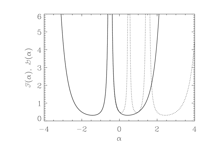
Figure 1: Amplitude of the magnetic power spectrum (solid line) at the end of inflation, as given by the function ${\cal F}(\alpha)$ defined in Eq. (38), in terms of the index $\alpha$ characterizing the shape of the gauge coupling. An almost scale-invariant power spectrum, $\beta\simeq-2$, has been assumed such that $\gamma\equiv\alpha(1+\beta)\simeq-\alpha$. The divergence at $\alpha=-1/2$ signals the transition between the two branches of the spectrum. The amplitude of the electric power spectrum at the end of inflation is also displayed (dotted line). As shown in the following, the amplitude is given by the function ${\cal G}(\alpha)$ defined in Eq. (100).

Finally, the Fourier energy density of the magnetic field (in other words, the energy density stored at a given scale $k$) can be expressed as

$$\frac{{\rm d}}{{\rm d}k}\rho_{{}_{B}}(\eta,k)=\frac{k^{3}}{2\pi^{2}}{\cal F}(\delta)\frac{1}{a^{4}}\left(\frac{k}{aH}\right)^{2\delta}\,,$$ (39)

where, again, $\delta=\gamma$ if $\gamma\leq 1/2$ and $\delta=1-\gamma$ if $\gamma\geq 1/2$.

2.2 The Coupling Function

In the previous section, we have derived the power spectrum of the magnetic field under the assumption that $f\propto a^{\alpha}$. The goal of this section is to obtain the explicit form of $f(\phi)$ for various single field models of inflation.

Let us start with power-law inflation since this is a situation where an exact solution is available. In this case, the inflaton potential is given by

$$V(\phi)=V_{0}\exp\left[-\sqrt{2\epsilon_{1}}\left(\phi-\phi_{0}\right)\right]\,,$$ (40)

where $\epsilon_{1}$ is the first slow-roll parameter and is constant. Here, $\phi$ is dimensionless and denotes the vacuum expectation value measured is units of $M_{G}$. Then, in conformal time, the explicit solution of the Einstein equations reads

$$a(\eta)=\ell_{0}\left|\eta\right|^{1+\beta}\,,\quad\phi(\eta)=\phi_{0}+\sqrt{2\epsilon_{1}}\left(1+\beta\right)\ln|\eta|\,,$$ (41)

with $\beta\leq-2$ and $\epsilon_{1}=(2+\beta)/(1+\beta)$. Therefore, we see that, in order to satisfy our requirement $f\propto a^{\alpha}$, we must choose the coupling function such that

$$f(\phi)\propto\exp\left[\frac{\alpha}{\sqrt{2\epsilon_{1}}}(\phi-\phi_{0})\right]\,.$$ (42)

This is a priori interesting since this is precisely the shape postulated by Ratra in Ref. [30]. We will examine in Sec. 4 whether we can design a well-motivated model which naturally gives this case.

Let us now consider the case of a general potential. In this case, no exact solution is available but the slow-roll approximation can be used. Indeed, combining the two slow-roll equations of motion

$$H^{2}\simeq\frac{1}{3}V(\phi)\,,\quad\frac{{\rm d}\phi}{{\rm d}t}\simeq-\frac{1}{3H}\frac{{\rm d}V}{{\rm d}\phi}\,,$$ (43)

one obtains

$$\frac{{\rm d}a}{a}=-V(\phi)\left(\frac{{\rm d}V}{{\rm d}\phi}\right)^{-1}{\rm d}\phi$$ (44)

The integration of this equation is possible by quadrature. This provides us with the function $a(\phi)$ from which we trivially determine the form of the coupling function. One obtains

$$f(\phi)\propto\exp\left[-\alpha\int^{\phi}\frac{V(\varphi)}{V^{\prime}(\varphi)}{\rm d}\varphi\right]\,.$$ (45)

The above expression gives the form of the coupling function for any slow-roll model in terms of a single quadrature. In the following, we apply this general formula to various slow-roll scenarios. Let us start with the case of large field models, namely

$$V(\phi)=M^{4}\phi^{p}\,,$$ (46)

for which we find the following coupling function

$$f(\phi)\propto\exp\left(-\frac{\alpha}{2p}\phi^{2}\right)\,.$$ (47)

Then, we can also consider the case of small-field and hybrid inflation where the potential can be written as

$$V(\phi)=M^{4}(1\pm\lambda\phi^{p})$$ (48)

where the (upper) plus sign corresponds to the hybrid case ($p=2$ being the theoretically favored value) while the (lower) minus sign gives the small field case, and $\lambda$ is a constant. The corresponding coupling function reads

$$f(\phi)\propto\exp\left[\mp\frac{\alpha\phi^{2-p}}{\lambda p(2-p)}-\frac{\alpha\phi^{2}}{2p}\right]\,.$$ (49)

The case $p=2$ must be treated separately. One obtains

$$f(\phi)\propto\phi^{\mp\alpha/(2\lambda)}\exp\left(-\frac{\alpha\phi^{2}}{4}\right)\,.$$ (50)

The case of small field is particularly interesting. Indeed, in this case, $\phi\ll m_{\scriptscriptstyle{\mathrm{Pl}}}$, and the exponential term can be neglected. As a result, one finds

$$f(\phi)\propto\phi^{\alpha/(2\lambda)}\,.$$ (51)

The question is now to see whether one can find high-energy particle physics models which reproduce the previous phenomenological approach. This will be studied in detail in Sec. 4.

2.3 The Magnetic Field during preheating

In this subsection, we study the behavior of the magnetic field during the preheating stage. Previously, we have determined the shape of the magnetic power spectrum and, in the following, we will evolve it until present time using a simple adiabatic law. However, one must first check that preheating is not going to affect either the amplitude or even the spectral shape of ${\rm d}\rho_{{}_{B}}/{\rm d}k$. During preheating, at least if the potential can be approximated by a parabola, the inflaton field behaves according to

$$\phi(t)\simeq\frac{\sqrt{8}}{\sqrt{3}mt}\sin\left(mt\right)\,.$$ (52)

In the following we work in terms of cosmic time since this is more convenient for our purpose. Then, the Fourier amplitude $A(t,k)$ obeys the equation

$$\ddot{A}(t,k)+\left(3H+2\frac{\dot{f}}{f}\right)\dot{A}(t,k)+\left(\frac{k^{2}}{a^{2}}+H^{2}+2H\frac{\dot{f}}{f}+\frac{\ddot{a}}{a}\right)A(t,k)=0\,.$$ (53)

Let us now consider the new rescaled variable $\aleph(t,k)$ defined by $A(t,k)=\aleph(t,k)a^{-3/2}(t)f^{-1}(t)$. We are led to introduce a new variable, slightly different from the one used before ${\cal A}(\eta,k)$, because we now work in terms of cosmic time rather than in conformal time. Using the above equation, it is straightforward to show that

$$\ddot{\aleph}(t,k)+\left(\frac{k^{2}}{a^{2}}-\frac{\ddot{f}}{f}-H\frac{\dot{f}}{f}+\frac{1}{4}H^{2}-\frac{1}{2}\frac{\ddot{a}}{a}\right)\aleph(t,k)=0\,.$$ (54)

In order to go further, one needs to know the time-behavior of $f(t)$ during preheating which requires the knowledge of the shape of the inflaton potential during this stage of evolution. In the simple approach considered here, this is the case only for chaotic inflation. Indeed, the shape of $V(\phi)$ used in the power-law case (40) or in the small field/hybrid case (48) is only valid during the slow-roll phase. Therefore, let us now concentrate on the case of chaotic inflation. In this case, using Eqs. (47) and (52) the coupling function is given by

$$f(t)\propto\exp\left[-\frac{4\alpha}{3p(mt)^{2}}\sin^{2}\left(mt\right)\right]\,.$$ (55)

From this expression, one can evaluate the time-dependence of the effective frequency in Eq. (54). For the term $\ddot{f}/f$, straightforward calculations lead to

$$\frac{\ddot{f}}{f} = \frac{4\alpha}{3pt^{2}}\left[-\frac{6}{(mt)^{2}}\sin^{2}(mt)+\frac{3}{mt}\sin(2mt)-2\cos(mt)\right]$$ (56)

$$+ \frac{16\alpha^{2}}{9p^{2}m^{2}t^{4}}\left[\frac{4}{(mt)^{2}}\sin^{4}(mt)-\frac{4}{mt}\sin^{3}(mt)+\sin^{2}(2mt)\right]\,,$$

$$= -\frac{8\alpha}{3pt^{2}}\cos(2mt)+{\cal O}\left(\frac{1}{mt^{3}}\right)\,.$$ (57)

As a consequence, Eq. (54) can be approximated as

$$\ddot{\aleph}(t,k)+\left[\frac{k^{2}}{a^{2}}+\frac{1}{4}H^{2}+\frac{8\alpha}{3pt^{2}}\cos(2mt)\right]\aleph(t,k)=0\,,$$ (58)

where we have retained the most and the least rapidly changing terms in the bracket in order to compare with the Mathieu equation, ${\rm d}^{2}\aleph/{\rm d}z^{2}+\left(a_{{}_{\rm M}}-2q_{{}_{\rm M}}\cos 2z\right)=0$. Then, defining $z\equiv mt-\pi/2$, Eq. (58) is rewritten as

$$\frac{{\rm d}^{2}\aleph}{{\rm d}z^{2}}+\left[\frac{k^{2}}{a^{2}m^{2}}+\frac{H^{2}}{4m^{2}}-\frac{8\alpha}{3p(z+\pi/2)^{2}}\cos 2z\right]\aleph=0\,.$$ (59)

So we find

$$a_{{}_{\rm M}}=\frac{k^{2}}{a^{2}m^{2}}+\frac{H^{2}}{4m^{2}}\,,\quad q_{{}_{\rm M}}=\frac{4\alpha}{3p(z+\pi/2)^{2}}\,,$$ (60)

for a time scale much shorter than the Hubble time. Since we are interested in the long wave modes and $H\ll m$, we find $a_{{}_{\rm M}}\ll 1$. Then, the Mathieu equation has instability only for $q_{{}_{\rm M}}\gtrsim 1$. Since both $\alpha$ and $p$ are constants of order unity with their typical values $\alpha=p=2$, we can conclude that the instability continues for less than one period of the field oscillation. The parametric resonance is therefore entirely negligible and we cannot expect any enhancement of the magnetic field during preheating, at least with the coupling function considered in this article.

2.4 The Magnetic Field after Inflation

After inflation and preheating, the Universe is full of charged particles and, therefore, the conductivity $\sigma_{\rm c}$ jumps up to a value much larger than the Hubble parameter almost abruptly. In this case, the model is described by the following action

$$S\left[A_{\mu}\right]=-\int{\rm d}^{4}x\sqrt{-g}\left(\frac{1}{4}g^{\alpha\beta}g^{\mu\nu}F_{\mu\alpha}F_{\nu\beta}-j^{\mu}A_{\mu}\right)\,,$$ (61)

where, now, the function $f=1$ since the inflaton field has decayed and is no longer present. The current $j^{\mu}$ is defined by the formula [43]

$$j_{\mu}=\rho_{\rm e}u_{\mu}+\sigma_{\rm c}E_{\mu}\,.$$ (62)

In this expression, $\rho_{\rm e}$ is the measurable charge density and $\sigma_{\rm c}$ is the scalar conductivity of the medium. The equation of motion now reads

$$-\frac{1}{\sqrt{-g}}\partial_{\mu}\left(\sqrt{-g}g^{\mu\nu}g^{\alpha\beta}F_{\nu\beta}\right)=j^{\alpha}\,,$$ (63)

and the new stress-energy tensor can be expressed as

$$T_{\mu\nu}=-g^{\alpha\beta}F_{\mu\alpha}F_{\beta\nu}-\frac{1}{4}g_{\mu\nu}g^{\alpha\beta}g^{\gamma\delta}F_{\beta\delta}F_{\alpha\gamma}+g_{\mu\nu}j_{\alpha}A^{\alpha}-2j_{\mu}A_{\nu}\,.$$ (64)

Then, the wave equation for the gauge field reads

$$\ddot{A_{i}}(t,{\mbox{\boldmath$x$\unboldmath}})+\left(\frac{\dot{a}}{a}+{\sigma}_{\mathrm{c}}\right)\dot{A_{i}}(t,{\mbox{\boldmath$x$\unboldmath}})-{\partial}^{j}{\partial}_{j}A_{i}(t,{\mbox{\boldmath$x$\unboldmath}})=0\,,$$ (65)

In the large scale limit (hence neglecting the spatial derivatives of the gauge field) and in the large conductivity limit, $\sigma_{\rm c}\gg H$, the solution to the above equation reads

$$A_{i}(t,{\mbox{\boldmath$x$\unboldmath}})=\frac{D_{1\,i}({\mbox{\boldmath$x$\unboldmath}})}{\sigma_{\rm c}}{\rm e}^{-\sigma_{\rm c}t}+D_{2\,i}({\mbox{\boldmath$x$\unboldmath}})\,,$$ (66)

The exponential term will die away very quickly (with a characteristic time $\tau=\sigma_{\rm c}^{-1}\gg 1/H$) and, therefore, one obtains $A_{i}(t,{\mbox{\boldmath$x$\unboldmath}})\simeq D_{2\,i}({\mbox{\boldmath$x$\unboldmath}})$. This implies that $E_{i}=0$ and $B_{i}$ is a constant in time. Let us now evaluate the energy density associated with the previous configuration. It is easy to see that the extra term coming from the current is given by $\rho=\sigma_{\rm c}A^{i}\dot{A}_{i}$ and therefore vanishes. At the end, only the magnetic part remains and reads

$$\rho_{{}_{\rm B}}=\frac{1}{4}\frac{1}{a^{4}}\delta^{ij}\delta^{k\ell}(\partial_{j}D_{2\,\ell}-\partial_{\ell}D_{2\,j})(\partial_{i}D_{2\,k}-\partial_{k}D_{2\,i})\propto\frac{1}{a^{4}}\,.$$ (67)

Therefore, after inflation and until present times, one expects $\rho_{{}_{B}}$ to scale as $1/a^{4}$ (independently of the era considered, ie radiation or matter). As a consequence, one deduces that the present magnetic energy density at a given scale $L$ can be expressed as

$$\rho_{{}_{B}}(z=0,L)=\frac{{\rm d}\rho_{{}_{B}}}{{\rm d}k}\left(z=z_{\rm end},k=\frac{2\pi}{L}\right)\frac{2\pi}{L}\left(\frac{a_{\rm end}}{a_{0}}\right)^{4}\,.$$ (69)

Using the expression of $\rho_{{}_{B}}$ at the end of inflation, one obtains, with the definition $\Omega_{{}_{B}}(k)\equiv\rho_{{}_{B}}(z=0,k)/\rho_{\rm cri}$,

$$\frac{{\rm d}\Omega_{{}_{B}}}{{\rm d}\ln k}=\frac{32}{9}{\cal F}(\delta)\left(\frac{\rho_{\rm cri}}{m_{\scriptscriptstyle{\mathrm{Pl}}}^{4}}\right)\left(\frac{\rho_{\rm cri}}{\rho_{\rm end}}\right)^{\delta}\left(\frac{a_{0}}{a_{\rm end}}\right)^{2\delta}\left(\frac{k}{a_{0}H_{0}}\right)^{2\delta+4}$$ (70)

To go further, one must therefore evaluate the ratio $a_{0}/a_{\rm end}$. Clearly, this ratio depends on all the history of the Universe, in particular, on the process on reheating. It has been shown in Refs. [46, 47] that it can be expressed as

$$\frac{a_{0}}{a_{\rm end}}=\frac{1}{R}\rho_{\rm end}^{1/2}\left(\Omega_{\rm rad}^{0}\right)^{-1/4}\left(3H_{0}^{2}\right)^{-1/4}\,,$$ (71)

where $H_{0}\simeq 2.1h\times 10^{-42}\mbox{GeV}$, $\Omega_{\rm rad}^{0}h^{2}\simeq 4.3\times 10^{-5}$, see Ref. [16], and the parameter $R$, which describes the reheating phase, is given by [46, 47]

$$\ln R \equiv \frac{1-3w_{\rm reh}}{3(1+w_{\rm reh})}\Biggl{[}\ln\left(g_{*}^{1/4}T_{\rm reh}\right)+\frac{1+3w_{\rm reh}}{2(1-3w_{\rm reh})}\ln\rho_{\rm end}$$ (72)

$$-\frac{1}{1-3w_{\rm reh}}\ln\left(\frac{3+3w_{\rm reh}}{5-3w_{\rm reh}}\right)-\ln\frac{30^{1/4}}{\sqrt{\pi}}\Biggr{]}\,.$$

This parameter depends, a priori, on three quantities: the reheating temperature, $T_{\rm reh}$, the equation of state during reheating, $w_{\rm reh}$, and the energy density at the end of slow-roll inflation, $\rho_{\rm end}$. However, if one considers a particular model then the number of free parameters can be reduced. For instance, in the case of large field models where $V(\phi)\propto\phi^{p}$, the equation of state during reheating is known, namely

$$w_{\rm reh}=\frac{p-2}{p+2}\,.$$ (73)

This leads to [46, 47]

$$\ln R = -\frac{p-4}{3p}\Biggl{[}\ln\left(g_{*}^{1/4}T_{\rm reh}\right)-\frac{p-1}{p-4}\ln\rho_{\rm end}$$ (74)

$$+\frac{p+2}{2(p-4)}\ln\left(\frac{3p}{p+8}\right)-\ln\frac{30^{1/4}}{\sqrt{\pi}}\Biggr{]}\,.$$

Moreover, the value of $\rho_{\rm end}$ can also be estimated. Indeed, the end of inflation is defined by the condition

$$\epsilon_{1}=-\frac{\dot{H}}{H^{2}}=\frac{3\dot{\phi}_{\rm end}^{2}/2}{\dot{\phi}_{\rm end}^{2}/2+V(\phi_{\rm end})}=1\,,$$ (75)

which implies that $\dot{\phi}_{\rm end}^{2}=V(\phi_{\rm end})$ or $\rho_{\rm end}=3V(\phi_{\rm end})/2$. Since $\phi_{\rm end}/m_{\scriptscriptstyle{\mathrm{Pl}}}=1/(2\sqrt{\pi})$ for the potential $V(\phi)=m^{2}\phi^{2}/2$, one obtains $\rho_{\rm end}\simeq 3m^{2}m_{\scriptscriptstyle{\mathrm{Pl}}}^{2}/(16\pi)$, the mass $m$ being known, thanks to the COBE/WMAP normalization. Straightforward calculations lead to $\rho_{\rm end}\sim 2160\pi^{2}/(2N_{*}+1)^{2}\times Q_{\rm rms-PS}^{2}/T^{2}\sim 1.03\times 10^{-11}$ with $Q_{\rm rms-PS}\simeq 6\times 10^{-6}$, $T\sim 2.7\mbox{K}$ and assuming that the number of e-folds between Hubble exit during inflation and the end of inflation is given by $N_{*}=50$. We conclude that, in the case of a massive large field model, the parameter $\ln R$ only depends on the reheating temperature.

The situation can be more complicated for other potentials. For small field models, the shape of the potential during the slow-roll phase is different from the shape of the potential during reheating. As a consequence, the equation of state $w_{\rm reh}$ cannot be computed from the parameters describing $V(\phi)$ as it was the case for large field models. It remains a free parameter. In the case of power law inflation and of hybrid inflation, one needs a mechanism of instability in order to stop inflation. Then, even $\rho_{\rm end}$ remains a free parameter since it is linked to the value of the inflaton field where the waterfall behavior starts. Reheating proceeds in a direction perpendicular (in the field space) to the inflationary valley and, therefore, requires the full set ($w_{\rm reh}$, $T_{\rm reh}$, $\rho_{\rm end}$) to be phenomenologically described.

Putting everything together one arrives at the following expression

$$\frac{{\rm d}\Omega_{{}_{B}}}{{\rm d}\ln k} = \frac{{\cal F}(\delta)}{18\pi^{2}}R^{-2\delta}(\Omega_{\rm rad}^{0})^{-\delta/2}\rho_{\rm cri}^{1+\delta/2}\left(\frac{k}{a_{0}H_{0}}\right)^{2\delta+4}\,,$$ (76)

$$\simeq 2.4\times 10^{-7}\left(2.28\times 10^{-58}\right)^{\delta+2}{\cal F}(\delta)R^{-2\delta}h^{2\delta+2}\left(\frac{k}{a_{0}H_{0}}\right)^{2\delta+4}\,.$$ (77)

This equation is one of the most important result of this article. It gives the amplitude, at a given scale, of the magnetic field today in terms of four parameters: $\delta$, $\rho_{\rm end}$, $T_{\rm reh}$ and $w_{\rm reh}$.

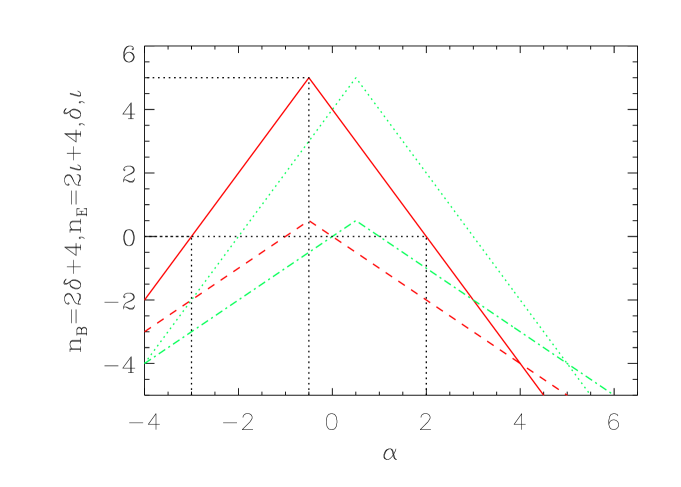
Figure 2: Spectral index $n_{{}_{B}}$ (solid red line) of the magnetic power spectrum as a function of the index $\alpha$, assuming, as before, a background expansion closed to de Sitter, i.e. $\beta\simeq-2$. Scale invariance of the magnetic power spectrum corresponds to the values $\alpha=2$ and $\alpha=-3$. The dashed red line represents the quantity $\delta$ (see the text) as a function of $\alpha$. The corresponding quantities for the electric field are also displayed, namely the spectral index $n_{{}_{E}}$ (green dotted line) and the function $\iota$ (green dotted-dashed line), see the definition of $\iota$ in the text after Eq. (100) and Eq. (101). Scale-invariance of the magnetic power spectrum corresponds to a spectral index of the electric power spectrum given by $n_{{}_{E}}=-2$ for $\alpha=-3$ and $n_{{}_{E}}=2$ for $\alpha=2$. Scale invariance of the electric power spectrum is realized for $\alpha=-2$ or $\alpha=3$.

In Fig. 2, we have represented the spectral index of the magnetic power spectrum, $n_{{}_{B}}\equiv 2\delta+4$ as a function of $\alpha$ as well as the quantity $\delta$ (see the red dashed line). The two branches of the spectrum are easily identified and meet at $\alpha=-1/2$. Scale invariance is obtained for $\alpha=2$ or $\alpha=-3$. For values of $\alpha$ such that $-3<\alpha<2$, we have a positive index, that is to say a blue spectrum while for $\alpha<-3$ and $\alpha>2$, we have a negative index i.e. a red spectrum.

In the next section, we find the constraints put on $\alpha$ by the currently available data on the magnetic power spectrum.

3 Constraining the coupling

3.1 Limits on Cosmological Magnetic Fields

Before comparing the above results with observation we summarize upper limits on cosmological magnetic fields from the following sources (see more detailed explanations in Refs. [3, 48]). The first type of constraints comes from CMB anisotropy measurements. Indeed, homogeneous magnetic fields during the time of decoupling whose scales are larger than the horizon at that time cause the Universe to expand at different rates in different directions. Since anisotropic expansion of this type distorts CMB, measurements of CMB angular power spectrum impose limits on the cosmological magnetic fields. Barrow, Ferreira, and Silk [49] carried out a statistical analysis based on the 4-year COBE data for angular anisotropy and derived the following limit on the primordial magnetic fields that are coherent on scale larger than the present horizon.

$$B_{\mathrm{cosmic}}^{(0)}<5\times 10^{-9}\mathrm{G}\,.$$ (78)

Moreover, in Ref. [50], a limit on primordial small-scale magnetic fields was obtained, also from CMB distortions. The constraint reads

$$B_{\mathrm{cosmic}}^{(0)}<3\times 10^{-8}\mathrm{G}\,,$$ (79)

for coherence lengths from $\sim 400\mathrm{pc}$ and $\sim 0.6\mathrm{Mpc}$.

Another type of constraint comes from Big Bang Nucleosynthesis (BBN) since magnetic fields that existed during the BBN epoch would affect the expansion rate, reaction rates, and electron density. Taking all these effects into account in calculation of the element abundances, and then comparing the results with the observed abundances, one can set limits on the strength of the magnetic fields. The limits on homogeneous magnetic fields on the BBN horizon size $\sim 1.4\times 10^{-4}\mathrm{Mpc}$ are such that

$$B_{\mathrm{cosmic}}^{(0)}<10^{-6}\mathrm{G}\,,$$ (80)

in terms of today’s values [51, 52].

Rotation Measure (RM) observations also provide interesting limits. RM data for high-redshift sources can be used to constrain the large-scale magnetic fields. For example, Vall$\acute{\mathrm{e}}$e [53] tested for an RM dipole in a sample of 309 galaxies and quasars. The galaxies in this sample extended to $z\simeq 3.6$ though most of the objects were at $z\lesssim 2$. Vall$\acute{\mathrm{e}}$e derived an upper limit of $6\times 10^{-10}{\left({n_{e}}_{0}/10^{-7}\mathrm{cm^{-3}}\right)}^{-1}\mathrm{G}$, where ${n_{e}}_{0}$ is the present mean density of thermal electrons, on the strength of uniform component of a cosmological magnetic field (${n_{e}}_{0}<{n_{b}}_{0}=(2.7\pm 0.1)\times 10^{-7}\mathrm{cm^{-3}}$, where ${n_{b}}_{0}$ is the current density of baryons [54]). Let us also notice that Ref. [55] also quotes limits obtained from Faraday measurements, namely

$$B_{\mathrm{cosmic}}^{(0)}<6\times 10^{-9}\mathrm{G}\,,$$ (81)

for scales $\sim 50\mathrm{Mpc}$ and

$$B_{\mathrm{cosmic}}^{(0)}<10^{-8}\mathrm{G}\,,$$ (82)

for coherence lengths corresponding to $\sim\mathrm{G}$.

Finally, one can also take into account a constraint which is of different nature. It is known [3] that the magnetic field on scales $\sim 1\mathrm{Mpc}$ must be

$$B_{\mathrm{cosmic}}^{(0)}>10^{-22}\mathrm{G}\,,$$ (83)

in order to ignite efficiently the dynamo mechanism at the galactic scales, as was also mentioned in Sec. 1. This constraint is clearly different from the above ones since it comes from a theoretical prejudice. However, it is interesting since this leads to a lower limit rather than upper bounds as discussed before.

These limits can be translated directly into limits on $\Omega_{{}_{B}}$. Indeed, the energy density associated with the magnetic field reads $\rho_{{}_{B}}=B^{2}/2$ (with our normalization of the gauge field kinetic term, see also Ref. [16]) and this implies ${\rm d}\Omega_{{}_{B}}/{\rm d}\ln k=4\pi B^{2}/(3H_{0}^{2}m_{\scriptscriptstyle{\mathrm{Pl}}}^{2})$. Since $1\mbox{T}^{2}/2\simeq 1.9\times 10^{-32}\mbox{GeV}^{4}$ and $1\mbox{T}=10^{4}\mbox{G}$, one arrives at

$$h^{2}\frac{{\rm d}\Omega_{{}_{B}}}{{\rm d}\ln k}\simeq 2.425\times 10^{6}\left(\frac{B}{1\mbox{G}}\right)^{2}\,.$$ (84)

All the constraints on the present amplitude of the magnetic field are summarized in Fig. 3.

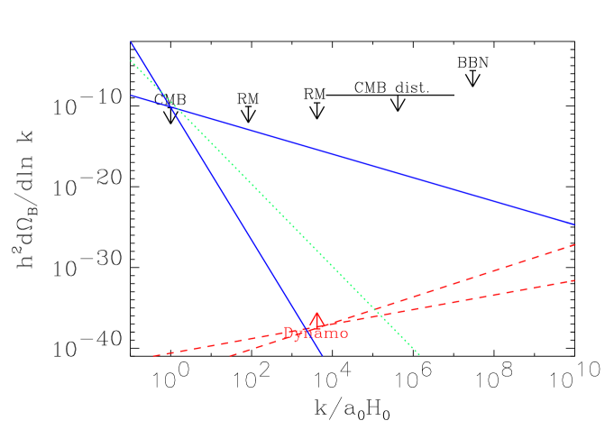
Figure 3: Constraints on the amplitude of the present-day magnetic field at different scales. The bounds come from CMB measurements, Big Bang nucleosynthesis (BBN) and Faraday rotation (RM). The dynamo theoretical constraint is also plotted. The two solid blue lines represent the reddest spectra compatible with the CMB constraint at the Hubble scale in the case of a general model of inflation and in the case of large field models, respectively, while the dotted green line is the reddest spectrum compatible with the CMB constraint and the dynamo limit (valid in the case of a general model). Finally, the two dashed red lines are the bluest spectra (for a general model and for large field, respectively) compatible with the dynamo constraint.

3.2 Constraining the Primordial Spectrum

In this section, our main goal is to constrain the parameter $\gamma$ using the experimental data reviewed in the previous subsection. However, as already mentioned, the amplitude of the theoretical spectrum given by Eq. (76) also depends on three other parameters, namely $w_{\rm reh}$, $T_{\rm reh}$, $\rho_{\rm end}$, that are not known precisely. Therefore, we first need to discuss the constraints existing on the values of those parameters.

Let us start with the limits on the parameters $R$. First of all, there are limits on $\rho_{\rm end}$ since, in order to preserve the success of the Big Bang Nucleosynthesis, one needs $\rho_{\rm end}>\rho_{\rm nuc}\simeq 10^{-85}m_{\scriptscriptstyle{\mathrm{Pl}}}^{4}$. On the other hand, one knows that the energy scale of inflation is constrained from above, namely $H_{\rm inf}/m_{\scriptscriptstyle{\mathrm{Pl}}}<1.3\times 10^{-5}$, see Ref. [46]. As a consequence, one must require that $\rho_{\rm end}<10^{-10}m_{\scriptscriptstyle{\mathrm{Pl}}}^{4}$. Summarizing the constraints, one has

$$-187<\ln\rho_{\rm end}<-20\,.$$ (85)

Let us now consider the equation of state during reheating, $w_{\rm reh}$. Reheating is, by definition, a phase of evolution where the scale factor does not accelerate which means that the strong and dominant energy conditions should be satisfied, that is to say

$$-\frac{1}{3}<w_{\rm reh}<1\,.$$ (86)

Finally, one also gets constraints on $\rho_{\rm reh}=g_{*}\pi^{2}T^{4}_{\rm reh}/30$ from the obvious requirement that reheating must proceed after the end of inflation and before the BBN, that is to say

$$\rho_{\rm nuc}<\rho_{\rm reh}<\rho_{\rm end}\,.$$ (87)

Taking everything into account, one arrives at the following model-independent range of variation

$$\frac{1}{4}\ln\rho_{\rm nuc}<\ln R<-\frac{1}{12}\ln\rho_{\rm nuc}+\frac{1}{3}\ln\rho_{\rm end}\,,$$ (88)

up to negligible factors depending on $w_{\rm reh}$ only. This leads to

$$-47\lesssim\ln R\lesssim 10\,.$$ (89)

In Ref. [46], CMB data have been used to constrain the values of $\ln R$ for large, small, hybrid and running mass inflationary scenarios. Some very weak limits have been obtained in the case of small field models but, essentially, the currently available data are not yet accurate enough and the marginalized probabilities obtained are just cut at the edges of their priors. Therefore, in absence of any other constraints, one must consider the interval given by Eq. (89). This is what is assumed here for power-law inflation even if, strictly speaking, the analysis on $\ln R$ should be redone for this model which was not explicitly considered in Ref. [46]. However, it seems extremely likely that no strong constraints would be obtained with the present-day data. In addition, let us recall that, in order to stop inflation, one must implement a mechanism of tachyonic instability where $\rho_{\rm end}$ is now viewed as a free parameter of the model. In this context, the constraint of Eq. (89) seems to be particularly relevant.

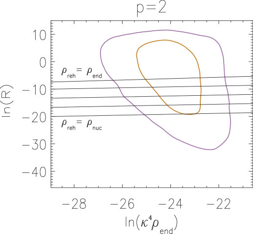
Figure 4: Constraints obtained from the WMAP3 data on the parameter $\ln R$ at $1\sigma$ and $2\sigma$, see Ref. [46]. The solid lines represent the variation of $\ln R$ as a function of the energy density at the end of inflation for various reheating temperatures (or, equivalently, for various energy densities at the end of reheating). No observational constraint on $T_{\rm reh}$ is obtained in the case of large field models.

As already mentioned, the situation is slightly different for the massive large field model, $p=2$. Indeed, in this case, the equation of state during reheating is known $w_{\rm reh}=0$, as well as $\rho_{\rm end}$ (at least approximatively, see above). In this case, one obtains the following constraint $-20\lesssim\ln R\lesssim-6$. In Fig. 4, one has reproduced this range of variation together with the constraints on $\ln R$ obtained by scanning general models of the form, $V(\phi)\propto\phi^{p}$, for more details see Ref. [46]. This plot confirms that the reheating temperature remains a free quantity with the currently available CMB data.

Let us now turn to the constraints on $\alpha$. In the case where the spectral index $n_{{}_{B}}$ is negative (red spectrum), the limiting constraint is the CMB constraint at scales of the order of the horizon today, see Fig. 3. So, one should require

$$\log_{10}\left(h^{2}\frac{{\rm d}\Omega_{{}_{B}}}{{\rm d}\ln k}\right)<\log_{10}\left(h^{2}\frac{{\rm d}\Omega_{{}_{B}}}{{\rm d}\ln k}\Biggl{|}_{{}_{\rm CMB}}\right)\simeq-10.2\,.$$ (90)

According to Fig. 2, $n_{{}_{B}}<0$ means either $\alpha>2$ or $\alpha<-3$. Looking at the dashed red line, one sees that this implies $\delta<0$ in these two regimes and for this reason, one writes $\delta=-|\delta|$. Then, using Eq. (76) and working out Eq. (90), one obtains

$$|\delta|<\frac{122.47+\log_{10}\left(h^{2}{\rm d}\Omega_{{}_{B}}/{\rm d}\ln k|_{{}_{\rm CMB}}\right)-\log_{10}{\cal F}-4\log_{10}\left[k/\left(a_{0}H_{0}\right)\right]}{57.92+0.86\ln R-2\log_{10}\left[k/\left(a_{0}H_{0}\right)\right]}\,,$$

where we have used $h\simeq 0.72$. In fact, this inequality is not as simple as it may seem since ${\cal F}$ is also a function of $\delta$. Therefore, given the functional form of ${\cal F}$, only a numerical calculation could allows us to derive the exact bound on $\delta$. However, the impact of the term $\log_{10}({\cal F})$ is limited and can be neglected in a first approximation. Moreover, since we seek an upper limit, it is clear from the above expression that the smallest value of $\ln R$ should be considered in order to reduce the denominator. According to the considerations presented before, this means $\ln R\sim-47$ in general and $\ln R\sim-26$ for large field models. Then, using $k/(a_{0}H_{0})=1$ and $\log_{10}\left(h^{2}{\rm d}\Omega_{{}_{B}}/{\rm d}\ln k|_{{}_{\rm CMB}}\right)\simeq-10.21$, one arrives at $|\delta|\lesssim 6.1$ and $|\delta|\lesssim 2.72$ for large fields. The corresponding spectra are represented in Fig. 3, see the two solid blue lines. If $\alpha>2$, then $\delta=-\alpha$ and the two bounds respectively correspond to $\alpha<6.1$ and $\alpha<2.72$. On the other hand, if $\alpha<-3$, then $\delta=1+\alpha$. As a consequence, one obtains $\alpha>-7.1$ and $\alpha>-3.72$. However, one notices in Fig. 3 that the spectra with $\alpha=6.1$ and $\alpha=-7.1$ violate the dynamo limit (this is not the case for large field models). Therefore, one should repeat the calculation and require the dynamo limit to be also satisfied. Straightforward calculations indicate that this amounts to $\alpha<4.55$ and $\alpha>-5.55$ (with, this time, $\ln R\sim-39.2$). The corresponding spectrum is represented in Fig. 3 by the dotted green line.

Let us now consider the case where we have a blue spectrum, $n_{{}_{B}}>0$. According to Fig. 3, this means $-3<\alpha<2$. This time the situation could be more complicated because this range of values can correspond to positive or negative values of $\delta$, see the dashed red line in Fig. 2. However, in practice, one remains in the regime where $\delta<0$ as will be checked below and, hence, $\delta=-|\delta|$. For blue spectra, the relevant constraint is the dynamo constraint which reads

$$|\delta|>\frac{78.23-\log_{10}{\cal F}}{50.68+0.86\ln R}\,,$$ (92)

where we have used

$$\log_{10}\left(h^{2}\frac{{\rm d}\Omega_{{}_{B}}}{{\rm d}\ln k}\Biggl{|}_{{}_{\rm Dynamo}}\right)\simeq-37.61\,,$$ (93)

and $\log_{10}[k/(a_{0}H_{0})]\sim 3.62$, the scale at which the dynamo constraint applies. Since we now seek a lower bound on $|\delta|$, one should use the largest value of $\ln R$, that is to say $\ln R\sim 10$ in general and $\ln R\sim-6$ for large field models. This respectively gives $|\delta|>1.19$ and $|\delta|>1.55$. This implies $\alpha>1.19$ and $\alpha>1.55$ in the case where $\alpha>-1/2$ (and, hence, one verifies that, for these values of $\alpha$, $\delta$ is indeed negative, see Fig. 2). In the other case, this means $\delta=1+\alpha<0$ and, therefore, one has $\alpha<-2.19$ and $\alpha<-2.55$. The corresponding spectra are represented in Fig. 3 by the two dashed red lines, the one with the smallest slope being the spectra in the case of large field models.

Summarizing all the results obtained above, one obtains the following general constraints

$$-5.55<\alpha<-2.19\,,\quad 1.19<\alpha<4.55\,,$$ (94)

while, for the case of large field models, one arrives at

$$-3.72<\alpha<-2.55\,,\quad 1.55<\alpha<2.73\,.$$ (95)

This means that, if $\alpha$ is in the above ranges of values, then there exists at least one value of $\ln R$ such that the corresponding spectrum is compatible with the currently available data.

3.3 Consistency and the Back-reaction Problem

We now evaluate the electric field produced in the model under investigation. Our goal in this subsection is to check that the total amount of magnetic and electric energy density produced during inflation is not larger than the background energy density $\sim H_{\rm inf}^{2}m_{\scriptscriptstyle{\mathrm{Pl}}}^{2}$. Otherwise, clearly, the framework used here would not be consistent and would suffer from a serious back-reaction problem. Using the expression of the stress-energy tensor, see Eq. (24), one obtains for the electric time-time component

$$T^{E}{}^{0}{}_{0}=-\frac{1}{2}\frac{f^{2}}{a^{2}}g^{ij}\partial_{0}A_{i}\partial_{0}A_{j}\,,$$ (96)

from which straightforward calculations lead to the following expression for the vacuum energy density

$$\left\langle T^{E}{}^{0}{}_{0}\right\rangle=-\frac{1}{2\pi^{2}}\frac{f^{2}}{a^{4}}\int{\rm d}kk^{2}\left|\left(\frac{{\cal A}}{f}\right)^{\prime}\right|^{2}\,,$$ (97)

or, in terms of electric energy density stored at the scale $k$

$$\frac{{\rm d}}{{\rm d}k}\rho_{{}_{E}}=\frac{f^{2}}{2\pi^{2}}\frac{k^{2}}{a^{4}}\left|\left[\frac{{\cal A}(k,\eta)}{f}\right]^{\prime}\right|^{2}\,.$$ (98)

This equation should be compared to Eq. (29). The solution for the Fourier amplitude of the vector potential has already been obtained previously in terms of Bessel functions. Using Eq. (34) on large scales compared to the Hubble radius, that is to say $k/(aH)=-k\eta\to 0$, one obtains

$${\cal A}^{\prime}-\frac{f^{\prime}}{f}{\cal A} \to \frac{\sqrt{\pi}}{2^{\gamma+3/2}}\frac{{\rm e}^{i\pi\gamma/2-i\pi}}{\Gamma(\gamma+3/2)\cos(\pi\gamma)}k^{1/2}(k\eta)^{\gamma+1}$$ (99)

$$+\frac{\sqrt{\pi}}{2^{-\gamma+1/2}}\frac{{\rm e}^{-i\pi(3+\gamma)/2}}{\Gamma(-\gamma+1/2)\cos\left[-\pi(1+\gamma)\right]}k^{1/2}(k\eta)^{-\gamma}\,,$$

where, as was already done for the magnetic field, the amplitude of the two modes has been written such that the symmetry $\gamma\to-1-\gamma$ is manifest. Clearly, this symmetry is not exactly similar to the one obtained in the magnetic case. Let us now define the dimensionless function ${\cal G}(\iota)$ by the following expression

$${\cal G}(\iota)\equiv\frac{\pi}{2^{2\iota+3}\Gamma^{2}(\iota+3/2)\cos^{2}(\pi\iota)}\,,$$ (100)

with $\iota=\gamma+1$ if $\gamma\leq-1/2$ and $\iota=-\gamma$ if $\gamma\geq-1/2$. This definition is very similar to the definition (38). The functions $\iota(\alpha)$ and ${\cal G}(\alpha)$ are represented in Figs. 2 and 1 respectively. With the help of ${\cal G}(\iota)$, we can write the Fourier energy density of the electric field. One obtains

$$\frac{{\rm d}}{{\rm d}k}\rho_{{}_{E}}(\eta,k)=\frac{k^{3}}{2\pi^{2}}{\cal G}(\iota)\frac{1}{a^{4}}\left(\frac{k}{aH}\right)^{2\iota}\,.$$ (101)

This expression should be compared to the formula expressing the magnetic energy density at a given scale $k$, see Eq. (39).

We are now in a position where one can estimate when a back-reaction problem occurs. Clearly, the model is free of this difficulty when the following condition is satisfied

$$\frac{{\rm d}\rho_{{}_{E}}}{{\rm d}\ln k}\biggl{|}_{\rm inf}+\frac{{\rm d}\rho_{{}_{B}}}{{\rm d}\ln k}\biggl{|}_{\rm inf}<\rho_{\rm inf}\,,$$ (102)

where, in the present context, the subscript “inf” means evaluated at the end of inflation. Indeed, as discussed previously, after the end of inflation, the conductivity jumps and, as a consequence, the gauge field becomes constant and, therefore, the electric field vanishes. Thus, if one checks that, at the end of inflation, the electric field can not cause a back-reaction problem, then we are guaranteed that the complete scenario is consistent. Let us also notice that the previous equation should be satisfied at any scales of astrophysical relevance today. Using the expression of the magnetic and electric energy densities derived before, the above relation amounts to

$$\frac{H_{\rm inf}^{4}}{2\pi^{2}}\Biggl{[}{\cal G}(\iota)\left(\frac{a_{0}H_{0}}{a_{\rm inf}H_{\rm inf}}\right)^{2\iota+4}\left(\frac{k}{a_{0}H_{0}}\right)^{2\iota+4}$$

$$+{\cal F}(\delta)\left(\frac{a_{0}H_{0}}{a_{\rm inf}H_{\rm inf}}\right)^{2\delta+4}\left(\frac{k}{a_{0}H_{0}}\right)^{2\delta+4}\Biggr{]}<\frac{3}{8\pi}H_{\rm inf}^{2}m_{\scriptscriptstyle{\mathrm{Pl}}}^{2}\,.$$ (103)

In the following, for simplicity, we will not distinguish the energy density at the end of inflation from the energy density at which the scales of astrophysical interest today left the Hubble scale. Clearly, this is a good approximation during inflation (almost by definition). Under this assumption, using Eq. (71), one can estimate the ratio $a_{0}H_{0}/(a_{\rm inf}H_{\rm inf})$ which enters the constraint (3.3). One obtains

$$\frac{a_{0}H_{0}}{a_{\rm inf}H_{\rm inf}}\simeq 1.51\times 10^{-29}\frac{h}{R}\,.$$ (104)

Therefore, one sees that the constraint (3.3) is quite difficult to analyze in full generality since, as already discussed, the quantity $R$ depends on three parameters, namely the energy density at the end of inflation, the equation of state parameter during reheating and the reheating temperature, see also Eq. (72). In the following, instead of performing a systematic scanning of the parameter space, we just show that, in the vicinity of the “scale-invariant” values $\alpha=-3$ and $\alpha=2$, there exist consistent models of inflation where the back-reaction problem does not occur. For this purpose, for simplicity, one first assumes instantaneous reheating, $g_{*}T_{\rm reh}^{4}\sim 90H_{\rm end}^{2}m_{\scriptscriptstyle{\mathrm{Pl}}}^{2}/(8\pi^{3})$. Then, the expression of $\ln R$ simplifies considerably and reads

$$\ln R\simeq\frac{1}{4}\ln\rho_{\rm end}\,.$$ (105)

Then it is straightforward to work out the constraint (3.3). For $\alpha=-3$, using Eqs. (104) and (105), one obtains

$$\frac{H_{\rm inf}}{m_{\scriptscriptstyle{\mathrm{Pl}}}}<{\cal O}(1)\times 10^{-20}\left(\frac{k}{a_{0}H_{0}}\right)^{2/3}\,.$$ (106)

Since, in the present situation, the magnetic power spectrum is scale invariant, the above constraint comes almost entirely from the requirement that the electric energy density should be less that the inflationary background energy density. Moreover, for $\alpha=-3$, one has a red electric power spectrum with $n_{{}_{E}}=-2$, see Fig. 2. As a consequence, if the above constraint is satisfied at the Hubble scale, $k/(a_{0}H_{0})\simeq 1$, then it is satisfied at any scales of astrophysical relevance today. Therefore, for the case $\alpha\sim-3$, one finds $H_{\rm inf}/m_{\scriptscriptstyle{\mathrm{Pl}}}\lesssim 10^{-20}$ or $\rho_{\rm inf}\sim 10^{-41}m_{\scriptscriptstyle{\mathrm{Pl}}}^{4}$ (let us recall that $\rho_{\rm nuc}\sim 10^{-85}m_{\scriptscriptstyle{\mathrm{Pl}}}^{4}$).

However, we still have to check that the previous models satisfy the constraints of figure 3. Indeed, we have shown before that, for indices $\alpha$ in the ranges (94), there is always a value of $\ln R$, compatible with the CMB data, such that the model is in agreement with the observations. However, we have not proven that the models are compatible for any values of $\ln R$ (this is clearly not the case) and, hence, since $\ln R$ is now fixed (for instance with $w_{\rm reh}=0$ and $H_{\rm inf}\sim 10^{-20}m_{\scriptscriptstyle{\mathrm{Pl}}}$, one has $\ln R\sim-21.77$) one must verify that there is no problem with the data. In fact, it turns out that these models do not satisfy the dynamo constraint because the magnetic field is too strongly damped after inflation. If we want to solve this problem, one has to consider a different type of reheating era. Clearly, the most favorable situation is when $w_{\rm reh}\sim 1$ since this is the situation where $B$ scales the more slowly given that $-1/3<w_{\rm reh}<1$, namely $B\propto t^{-2/3}$ and when the reheating stage is prolonged as much as possible, that is to say down to a reheating temperature of the order of few MeV’s. In this case avoiding the back-reaction problem requires $H_{\rm inf}<10^{-22}m_{\scriptscriptstyle{\mathrm{Pl}}}$ which leads to $\ln R\sim-16.74$. The corresponding situation is illustrated in Fig. 5. This time, for the previous value of $\ln R$, one can check that the branch $\alpha=-3$ of the spectrum is still compatible with the dynamo constraint. Therefore, at least for this type of reheating period, this branch is still a viable alternative.

Figure 5: Inflationary (solid line), magnetic (dashed line) and electric (dotted line) energy densities at the end of inflation in the case where $\alpha=-3$, $H_{\rm inf}/m_{\scriptscriptstyle{\mathrm{Pl}}}=10^{-22}$ $n_{{}_{B}}=0$ and $n_{{}_{E}}=-2$. This situation corresponds to the limiting case treated in the text where there is no back-reaction problem, the electric energy density being always below the background energy density and where the dynamo constraint is still satisfied.

The case $\alpha\sim 2$ can be worked out in the same manner. Straightforward calculations lead to

$$\frac{H_{\rm inf}}{m_{\scriptscriptstyle{\mathrm{Pl}}}}<{\cal O}(1)\times 10^{58}\left(\frac{k}{a_{0}H_{0}}\right)^{-2}\,.$$ (107)

This time the electric spectral index is positive, $n_{{}_{E}}=2$ and, therefore, the power spectrum is blue. As consequence, one should check that the consistency relation (3.3) is satisfied at small scales, say $k/(a_{0}H_{0})\sim 10^{10}$. As is obvious from the above relation, this is very easily the case.

The fact that back-reaction is always satisfied when $\alpha\sim 2$ while it requires low scale inflation in the case $\alpha\sim-3$ can be easily understood, see also Ref. [39]. Indeed, from Eq. (20), one has $A_{i}(\eta,{\mbox{\boldmath$x$\unboldmath}})\sim\epsilon_{i\lambda}A(\eta,k)\sim{\cal A}(\eta,k)/f(\eta)$, where we have used the fact that the covariant polarization vector contains a factor $a(\eta)$, see Eq. (18). Then, from Eq. (21), one has the two following modes on larges scales ${\cal A}\propto f(\eta)$ and ${\cal A}\propto f(\eta)\int^{\eta}{\rm d}\tau/f^{2}(\tau)$. Clearly, from the above equations, the first mode leads to $A_{i}\sim\mbox{Const.}$ and, therefore, to a vanishing electric field, while the second remains time-dependent and can be responsible for the production of a strong electric field. Indeed, it is easy to see that, in this last case, $A_{i}(\eta,{\mbox{\boldmath$x$\unboldmath}})\propto a^{-1-2\alpha}$, that is to say $A_{i}(\eta,{\mbox{\boldmath$x$\unboldmath}})\propto a^{5}$ for $\alpha\sim-3$ and $A_{i}(\eta,{\mbox{\boldmath$x$\unboldmath}})\propto a^{-5}$ for $\alpha\sim 2$. Therefore, this mode is sub-dominant for $\alpha\sim 2$ but is dominant for the other branch of the spectrum $\alpha\sim-3$. In this case, its strong time-dependence $\propto a^{5}$ produces a strong electric field and this explains why the back-reaction problem can be severe in this situation. This problem can be avoided if the production of the electric field is limited as it happens to be the case if inflation proceeds at low scale.

4 Particle Physics Models

4.1 Power Law Inflation

In this section, we finally turn to the model-building issue. More precisely, the question addressed in this subsection is whether there is a natural high energy model with an exponential inflaton potential and an exponential gauge coupling, as was obtained in Sec. 2.2. We will consider the other models in the next subsections. In order to study this issue, let us consider that the inflaton field is a modulus field $T$ in string theory. Then, its Kähler and super potential are given by

$$K=-p\ln\left(T+T^{\dagger}\right)\,,\quad W=-\frac{M^{3}}{n}T^{n}\,,$$ (108)

the natural choice being $p=3$ (no-scale). Moreover, in string theory, a natural choice is $f(T)=T^{q}$ with the preferred choice $q=1$ [41]. Therefore, at first sight, this does not give the required $f$ function. However, one has to remember that the field $T$ is not canonically normalized because the Kähler potential is non-trivial. The canonical field $\phi$ is given by

$$T={\rm e}^{-\sqrt{2/p}\phi}\,.$$ (109)

As a consequence, one obtains a coupling function with the required exponential shape, namely

$$f(\phi)\propto{\rm e}^{-q\sqrt{2/p}\phi}\,.$$ (110)

Moreover, the F-term potential is also easily computed and one also obtains the required shape, namely an exponential dependence. The explicit expression reads

$$V\left(\phi\right)=\frac{M^{6}(n-3)}{6n}\exp\left[-\left(2n-3\right)\sqrt{\frac{2}{3}}\phi\right]\,.$$ (111)

If we compare the two previous formulas to Eqs. (42) and (40), then one obtains the correct power-law model for the choice

$$n=\frac{3}{2}\left(1+\sqrt{\frac{\epsilon_{1}}{3}}\right)\,,\quad q=-\frac{\alpha}{2}\sqrt{\frac{p}{\epsilon_{1}}}\,.$$ (112)

In particular, we see that the branch $\alpha\sim 2$ leads to a negative power for $q$ while the branch $\alpha\sim-3$ gives $q=3\sqrt{3}/(2\sqrt{\epsilon_{1}})\gg 1$. This is already an indication that it is difficult to reconcile the branch $\alpha\sim 2$ with a sensible model building. In fact, in the present context, even the $\alpha\sim-3$ branch cannot lead to the string inspired favored model with $q=1$. But, the lethal flaw of the above model is that the required value of $n$ is less than $3$ leading to a negative inflaton potential.

The next question is whether the mechanism of assisted inflation [56] could solve this situation. Let us envisage a situation where we have $N$ moduli such that

$$K=-\sum_{i=1}^{N}p_{i}\ln\left(T_{i}+T_{i}^{\dagger}\right)\,,\quad W=-\sum_{i=1}^{N}\frac{M^{3}}{n_{i}}T_{i}^{n_{i}}\,,$$ (113)

the no-scale structure being preserved if $\sum_{i=1}^{N}p_{i}=3$. As before, the field $T_{i}$ are not canonically normalized, the normalized field $\phi_{i}$ being given by

$$T_{i}={\rm e}^{-\sqrt{2/p_{i}}\phi_{i}}\,.$$ (114)

Straightforward manipulations lead to the following potential

$$V = \frac{M^{6}}{2}\exp\left(\sum_{i=1}^{N}\sqrt{2p_{i}}\phi_{i}\right)\Biggl{[}-\sum_{j=1}^{N}\sum_{k=1}^{N}\frac{1}{n_{k}}\exp\Biggl{(}-n_{j}\sqrt{\frac{2}{p_{j}}}\phi_{j}$$ (115)

$$-n_{k}\sqrt{\frac{2}{p_{k}}}\phi_{k}\Biggr{)}+\sum_{j=1}^{N}\frac{1}{p_{j}}\exp\left(-2n_{j}\sqrt{\frac{2}{p_{j}}}\phi_{j}\right)\Biggr{]}$$

If one considers the case of one field (which implies $p=3$), then one can check that Eq. (111) is correctly recovered. Then, let us consider that we have $N$ fields such that $p_{i}=3/N$ and $n_{i}=n$ for any index $i$. Then, the potential becomes

$$V(\phi)=\frac{M^{6}N^{2}(n-3)}{6n}\exp\left[-\left(2n-3N\right)\sqrt{\frac{2N}{3}}\phi\right]\,.$$ (116)

This implies that

$$n=\frac{3N}{2}\left(1+\frac{1}{N^{3/2}}\sqrt{\frac{\epsilon_{1}}{3}}\right)\,.$$ (117)

We see that $N\geq 2$ allows us to have a positive potential and, therefore, represents a meaningful model. Of course, the fact that the power of the superpotential is not an integer is not a nice feature and, for this reason, the model remains unsatisfactory. What about the gauge coupling? In presence of several superfields, the form of $f$ that should be chosen remains unclear. If we postulate that it depends on one superfield only (say the field $\phi_{i}$), then one gets

$$q=-\frac{\alpha}{2}\sqrt{\frac{p_{i}}{\epsilon_{1}}}\,,$$ (118)

In this case, and contrary to the single field case, $q$ is not necessarily very large (as one might think since it scales as the inverse of the slow-roll parameter) because $p_{i}$ can be a small number. In the case envisaged above, this is generically the case because $p_{i}=3/N$ (remember that only the condition $\sum_{i=1}^{N}p_{i}=3$ must be fulfilled in order to preserve the no-scale structure). Moreover, one could also imagine a case where all the coefficients $p_{i}$ are not equal. If one of the $p_{i}$ is relatively small, then it could compensate the inverse of the slow-roll parameter in order to give a number of order one. For the branch $\alpha\sim 2$, $q$ is negative and we are not aware of any well-motivated SUGRA model where this happens. Therefore, the most interesting case seems to use the other branch of the spectrum with $\alpha\sim-3$. Then, one obtains

$$q\sim\frac{|\alpha|}{2}\sqrt{\frac{3}{N\epsilon_{1}}}\,,$$ (119)

with $|\alpha|\sim 3$ and the favored model $q=1$ is obtained for

$$N\sim\frac{3\alpha^{2}}{4}\frac{1+\beta}{2+\beta}\,.$$ (120)

Of course $N$ should be an integer and this can be the case if $\alpha$ is not exactly $-3$. We have seen that this situation is perfectly compatible with the data, see the previous section. Let us give an example for the sake of illustration. We can take $\beta\sim-2.025$ leading the spectral index $n_{\scriptscriptstyle{\mathrm{S}}}=0.95$. Then, the value $\alpha=-3.00135$ gives $N=277$ fields in the model.

A last remark is in order here. We have seen that the branch $\alpha\sim-3$ is a viable solution only if the scale of inflation is low and the reheating stage quite long. Here, we can certainly design a model where this is the case since, in order to stop inflation, one needs to rely on a mechanism of tachyonic instability as in the case of hybrid inflation. In this situation, the energy density at the end of inflation remains a free parameter and can be chosen such that it leads to the correct scale of inflation. Moreover, the details of the reheating will depend of the shape of the potential in the direction perpendicular to the inflationary valley.

4.2 Large Field Inflation

One can generate large-scale magnetic field in large field inflation models if gauge kinetic function has appropriate dependence on the inflaton field given by Eq. (47). As the model of inflation we adopt a chaotic inflation in supergravity based on a shift symmetry $\Phi\longrightarrow\Phi+iC$ where $C$ is a real number. Specifically we adopt a model proposed in Ref. [57] with two chiral superfields $\Phi$ and $X$. In this model by virtue of this symmetry and its soft breaking, the Kähler potential and superpotential are given by

$$K=\frac{1}{2}(\Phi+\Phi^{\ast})^{2}+XX^{\ast}+\cdots\,,\quad W=mX\Phi,$$ (121)

where $m$ is a constant corresponding to the inflaton mass. The scalar Lagrangian possesses standard kinetic terms and is given by

$${\mathcal{L}}_{\mathrm{scalar}}=-\partial_{\mu}\Phi\partial^{\mu}\Phi^{\ast}-\partial_{\mu}X\partial^{\mu}X^{\ast}-V(\Phi,X)\,,$$ (122)

where the potential reads

$$V(\Phi,X) = m^{2}{\rm e}^{K}\Biggl{\{}|\Phi|^{2}\left(1+|X|^{4}\right)$$ (123)

$$+|X|^{2}\left[1-|\Phi|^{2}+\left(\Phi+\Phi^{\ast}\right)^{2}\left(1+|\Phi|^{2}\right)\right]\Biggr{\}}\,.$$

Decomposing the complex scalar field $\Phi$ into two real scalar fields as $\Phi=(\sigma+i\phi)/\sqrt{2}$ and using the fact that only $\phi$ can have a large initial value beyond the Planck scale without any exponential barrier due to the Kähler potential, we find that the Universe evolves as in the chaotic inflation model with a massive scalar field [58], namely

$${\mathcal{L}}_{\mathrm{inflaton}}=-\frac{1}{2}\partial_{\mu}\phi\partial^{\mu}\phi-V(\phi)\,,\quad V(\phi)=\frac{1}{2}m^{2}\phi^{2}\,.$$ (124)

Therefore, as announced, one has obtained the potential (46) with $p=2$. Here, we recall that all models such that $p>3.1$ are now excluded at $95\%$ confidence level by the WMAP3 data, see Ref. [46].

We now consider the vector part of the Lagrangian. Specifically we take the following Lagrangian for the U(1) gauge field

$${\mathcal{L}}_{{}_{\mathrm{EM}}}=-\frac{1}{4}\Re\tilde{f}(\Phi)F_{\mu\nu}F^{\mu\nu}\,,$$ (125)

with

$$\tilde{f}(\Phi)\equiv f_{0}{\rm e}^{\alpha\Phi^{2}}\,,$$ (126)

where $\alpha$ is a constant. Note that the shift symmetry of the system is preserved if $F_{\mu\nu}=0$. As argued above, since $\sigma$ rapidly relaxes to the origin at the onset of inflation, the gauge kinetic function then reduces to

$$\Re\tilde{f}(\Phi)=f_{0}{\rm e}^{-\alpha\phi^{2}/2}\equiv f^{2}(\phi)\,,$$ (127)

and it reproduces the coupling function given by Eq. (47) when $p=2$. However, and contrary to the case of power-law inflation, the choice (126) can no longer be justified from string theory, at least for the simple favored case mentioned before.

4.3 Small Field Inflation

Generation of large-scale magnetic field is also possible in small field inflation models. Here we adopt a model proposed in Ref. [59] which does not require fine tuning of the initial conditions. This model is based on the following Kähler potential and the superpotential

$$K=\frac{1}{2}(\Phi+\Phi^{\ast})^{2}+XX^{\ast}\,,\quad W=v^{2}X\left(1-g\Phi^{2}\right)\,.$$ (128)

Symmetry argument to obtain the above expression has been fully described in Ref. [59] and we do not repeat it here. In this model the real part of the scalar component $\Phi\equiv(\phi+i\chi)/\sqrt{2}$ plays the role of the inflaton for the small field inflation while its imaginary part serves as that for chaotic inflation which occurs beforehand. The quantity $X$ is another chiral superfield introduced to yield an appropriate scalar potential. The scalar part of the Lagrangian then reads

$$\mathcal{L}(\phi,\chi,X)=\frac{1}{2}\partial_{\mu}\phi\partial^{\mu}\phi+\frac{1}{2}\partial_{\mu}\chi\partial^{\mu}\chi+\partial_{\mu}X\partial^{\mu}X^{*}-V(\phi,\chi,X)\,,$$ (129)

with the potential $V(\phi,\chi,X)$ given by the following expression

$$V(\phi,\chi,X) = v^{4}{\rm e}^{|X|^{2}+\phi^{2}}\Biggl{\{}\left[\left(1-\frac{g}{2}\phi^{2}\right)^{2}+g\chi^{2}\left(1+\frac{g}{2}\phi^{2}+\frac{g}{4}\chi^{2}\right)\right]$$ (130)

$$\times\left(1-|X|^{2}+|X|^{4}\right)+|X|^{2}\Biggl{[}2g^{2}\chi^{2}+2(g-1)^{2}\phi^{2}$$

$$+2g\left(g+1\right)\phi^{2}\chi^{2}+2g\left(g-1\right)\phi^{4}+\frac{g^{2}}{2}\phi^{2}\left(\phi^{2}+\chi^{2}\right)^{2}\Biggr{]}\Biggr{\}}\,.$$

Since $\chi$ is free from exponential rise as in the model discussed in the previous subsection it can naturally induce chaotic inflation. Meanwhile $\phi$ and $X$ settle to the origin apart from quantum fluctuations. After chaotic inflation $\phi$ is still close to the origin and then induces new inflation. In this regime with $\chi=|X|=0$ and $|\phi|\ll 1$, the scalar potential reads

$$V(\phi)=v^{4}\left(1-\frac{c}{2}\phi^{2}\right),$$ (131)

with $c\equiv 2(g-1)$. Thus, if $g\gtrsim 1$, $\phi$ rolls down slowly toward the vacuum expectation value $\phi_{0}\equiv\sqrt{2/g}$ and small field inflation takes place. The potential (131) has the same form as (48).

Finally, using Eq. (51), the desired form of the gauge kinetic function is realized if we take

$$\tilde{f}(\Phi)\equiv f_{0}\Phi^{2\alpha/c}\,.$$ (132)

The branch $\alpha\sim 2$ is the one to be used in order to obtain positive $q$. The favored string inspired model $q=1$ is obtained for $c\simeq 4$ or $g\simeq 3$. However, unfortunately, this value is not compatible with the CMB constraints. Indeed, in the case of small field models, the first slow-roll parameter $\epsilon_{1}$ is exponentially small while the second one is given by $\epsilon_{2}=2c$, see Ref. [46]. The CMB constraints on $\epsilon_{2}$ are $-0.07<\epsilon_{2}<0.07$ at $95\%$ CL, see Ref. [46], which implies $-0.035<c<0.035$. This means that $q\gtrsim 57$, a value not compatible with the string inspired value and too large to be considered as natural. However, at the same time, the model makes use of the branch where the back-reaction problem is not severe at all. In this case, the characteristics of the required reheating stage seems easy to satisfy.

5 Conclusion

In this section, we recap our main results and discuss issues that should be studied in future works. In the present paper, we have studied the generation of large-scale magnetic fields in inflationary cosmology, breaking the conformal invariance of the electromagnetic field by introducing a coupling with the inflaton field as it is generic in a supergravity framework. We have determined the form of the coupling necessary in order to produce large-scale magnetic fields with the required strengths on the relevant astrophysical scales. We have shown that the scale-dependent magnetic energy density possess two branches. Among these two branches, one ($\alpha\sim-3$) seems to lead to sensible model building in the case of power-law inflation but only at the expense of having a low energy inflation scale and a long reheating stage. The other branch ($\alpha\sim 2$) is useful in the case of small field models and this case appears to be relevant since this does not require to fine-tune the reheating epoch. However, the model building condition $q\gtrsim 57$ cannot be justified in a string inspired model and seems artificial. Finally, in the context of large field models, we have shown that the required coupling is quite difficult to justify.

Determining exactly all the consistent models in the framework envisaged here is a non-trivial issue because the parameter space is large (at least four-dimensional), in particular when a general reheating stage is considered. Here, we have just proven that consistent models exist. However, it would certainly be interesting to systematically explore the parameter space in order to have a more accurate idea of whether the consistent models are just peculiar or, on the contrary, quite generic. Another interesting avenue for the future is clearly the model building issue. Here, we have noticed that the branch $\alpha\sim 2$ can be used only in the context of small field models. It would be interesting to find other models where this can also been done. We hope that these issues will be addressed in the near future.

References

References

- [1] P. P. Kronberg, Extragalactic magnetic fields, Rept. Prog. Phys. 57 (1994) 325–382.
- [2] D. Grasso and H. R. Rubinstein, Magnetic fields in the early universe, Phys. Rept. 348 (2001) 163–266, [astro-ph/0009061].
- [3] L. M. Widrow, Origin of galactic and extragalactic magnetic fields, Rev. Mod. Phys. 74 (2003) 775–823, [astro-ph/0207240].
- [4] Y. Sofue, M. Fujimoto, and R. Wielebinski, Global structure of magnetic fields in spiral galaxies, Ann. Rev. Astron. Astrophys. 24 (1986) 459–497.
- [5] P. P. Kronberg, J. J. Perry, and E. L. H. Zukowski, Discovery of extended farady rotation compatible with spiral structure in an intervening galaxy at z=0.395- new observations of pks 1229 - 021, Astrophys. J. 387 (1992) 528–535.
- [6] K. T. Kim, P. P. Kronberg, P. E. Dewdney, and T. L. Landecker, The halo and magnetic field of the coma cluster of galaxies, Astrophys. J. 355 (1990) 29–37.
- [7] K. T. Kim, P. P. Kronberg, and P. C. Tribble, Detection of excess rotation measure due to intracluster magnetic fields in clusters of galaxies, Astrophys. J. 379 (1991) 80–88.
- [8] T. E. Clarke, P. P. Kronberg, and H. Bohringer, A new radio-x-ray probe of galaxy cluster magnetic fields, Astrophys. J. 547 (2001) L111–L114.
- [9] E. N. Parker, The generation of magnetic fields in astrophysical bodies. ii. the galactic field, Astrophys. J. 163 (1971) 255–265.
- [10] E. N. Parker, Cosmical Magnetic Field. Clarendon, Oxford, England, 1979.
- [11] Y. B. Zel’dovitch, A. A. Ruzmaikin, and D. D. Sokoloff, Magnetic Fields in Astrophysics. Gordon and Breach, New York, 1983.
- [12] A. H. Guth, The inflationary universe: A possible solution to the horizon and flatness problems, Phys. Rev. D23 (1981) 347–356.
- [13] K. Sato, First order phase transition of a vacuum and expansion of the universe, Mon. Not. Roy. Astron. Soc. 195 (1981) 467–479.
- [14] A. D. Linde, Particle physics and inflationary cosmology, Contemp. Concepts Phys. 5 (2005) 1–362, [hep-th/0503203].
- [15] K. A. Olive, Inflation, Phys. Rept. 190 (1990) 307–403.
- [16] E. Kolb and M. Turner, The Early Universe, vol. 69 of Frontiers in Physics Series. Addison-Wesley Publishing Company, 1990.
- [17] D. H. Lyth and A. Riotto, Particle physics models of inflation and the cosmological density perturbation, Phys. Rept. 314 (1999) 1–146, [hep-ph/9807278].
- [18] J. Martin, Inflation and precision cosmology, Braz. J. Phys. 34 (2004) 1307–1321, [astro-ph/0312492].
- [19] J. Martin, Inflationary cosmological perturbations of quantum- mechanical origin, Lect. Notes Phys. 669 (2005) 199–244, [hep-th/0406011].
- [20] J. Martin, Inflationary perturbations: The cosmological schwinger effect, 0704.3540.
- [21] V. F. Mukhanov and G. V. Chibisov, Quantum fluctuation and ’nonsingular’ universe. (in russian), JETP Lett. 33 (1981) 532–535.
- [22] S. W. Hawking, The development of irregularities in a single bubble inflationary universe, Phys. Lett. B115 (1982) 295.
- [23] A. A. Starobinsky, Dynamics of phase transition in the new inflationary universe scenario and generation of perturbations, Phys. Lett. B117 (1982) 175–178.
- [24] A. H. Guth and S. Y. Pi, Fluctuations in the new inflationary universe, Phys. Rev. Lett. 49 (1982) 1110–1113.
- [25] L. P. Grishchuk, Amplification of gravitational waves in an isotropic universe, Sov. Phys. JETP 40 (1975) 409–415.
- [26] V. A. Rubakov, M. V. Sazhin, and A. V. Veryaskin, Graviton creation in the inflationary universe and the grand unification scale, Phys. Lett. B115 (1982) 189–192.
- [27] L. Parker, Particle creation in expanding universes, Phys. Rev. Lett. 21 (1968) 562–564.
- [28] M. S. Turner and L. M. Widrow, Inflation produced, large scale magnetic fields, Phys. Rev. D37 (1988) 2743.
- [29] B. Ratra, Inflation generated cosmological magnetic field, . CALT-68-1751.
- [30] B. Ratra, Cosmological ’seed’ magnetic field from inflation, Astrophys. J. 391 (1992) L1–L4.
- [31] D. Lemoine and M. Lemoine, Primordial magnetic fields in string cosmology, Phys. Rev. D52 (1995) 1955–1962.
- [32] M. Giovannini, On the variation of the gauge couplings during inflation, Phys. Rev. D64 (2001) 061301, [astro-ph/0104290].
- [33] M. Giovannini, Inflationary magnetogenesis from dynamical gauge couplings, hep-ph/0104214.
- [34] M. Giovannini, Magnetogenesis, variation of gauge couplings and inflation, astro-ph/0212346.
- [35] E. A. Calzetta, A. Kandus, and F. D. Mazzitelli, Primordial magnetic fields induced by cosmological particle creation, Phys. Rev. D57 (1998) 7139–7144, [astro-ph/9707220].
- [36] A. Kandus, E. A. Calzetta, F. D. Mazzitelli, and C. E. M. Wagner, Cosmological magnetic fields from gauge mediated supersymmetry-breaking models, Phys. Lett. B472 (2000) 287, [hep-ph/9908524].
- [37] A.-C. Davis, K. Dimopoulos, T. Prokopec, and O. Tornkvist, Primordial spectrum of gauge fields from inflation, Phys. Lett. B501 (2001) 165–172, [astro-ph/0007214].
- [38] A. Dolgov, Breaking of conformal invariance and electromagnetic field generation in the universe, Phys. Rev. D48 (1993) 2499–2501, [hep-ph/9301280].
- [39] K. Bamba and J. Yokoyama, Large-scale magnetic fields from inflation in dilaton electromagnetism, Phys. Rev. D69 (2004) 043507, [astro-ph/0310824].
- [40] K. Bamba and J. Yokoyama, Large-scale magnetic fields from dilaton inflation in noncommutative spacetime, Phys. Rev. D70 (2004) 083508, [hep-ph/0409237].
- [41] D. Bailin and A. Love, Supersymmetric Gauge Field Theory and String Theory. Graduent Student Series in Physics. Institute of Physics Publishing, Bristol and Philadelphia, 1994.
- [42] E. Cremmer, S. Ferrara, L. Girardello, and A. Van Proeyen, Yang-mills theories with local supersymmetry: Lagrangian, transformation laws and superhiggs effect, Nucl. Phys. B212 (1983) 413.
- [43] J. D. Barrow, R. Maartens, and C. G. Tsagas, Cosmology with inhomogeneous magnetic fields, Phys. Rept. 449 (2007) 131–171, [astro-ph/0611537].
- [44] J. Martin and D. J. Schwarz, The precision of slow-roll predictions for the cmbr anisotropies, Phys. Rev. D62 (2000) 103520, [astro-ph/9911225].
- [45] I. S. Gradshteyn and I. M. Ryzhik, Table of Integrals, Series, and Products. Academic Press, New York and London, 1965.
- [46] J. Martin and C. Ringeval, Inflation after wmap3: Confronting the slow-roll and exact power spectra to cmb data, JCAP 0608 (2006) 009, [astro-ph/0605367].
- [47] L. Lorenz, J. Martin, and C. Ringeval, Brane inflation and the wmap data: a bayesian analysis, 0709.3758.
- [48] T. Kollat, Determination of the primordial field power spectrum by farady rotation correlations, Astrophys. J. 495 (1998) 564.
- [49] J. D. Barrow, P. G. Ferreira, and J. Silk, Constraints on a primordial magnetic field, Phys. Rev. Lett. 78 (1997) 3610–3613, [astro-ph/9701063].
- [50] K. Jedamzik, V. Katalinic, and A. V. Olinto, A limit on primordial small-scale magnetic fields from cmb distortions, Phys. Rev. Lett. 85 (2000) 700–703, [astro-ph/9911100].
- [51] D. Grasso and H. R. Rubinstein, Revisiting nucleosynthesis constraints on primordial magnetic fields, Phys. Lett. B379 (1996) 73–79, [astro-ph/9602055].
- [52] B.-l. Cheng, A. V. Olinto, D. N. Schramm, and J. W. Truran, Constraints on the strength of primordial magnetic fields from big bang nucleosynthesis revisited, Phys. Rev. D54 (1996) 4714–4718, [astro-ph/9606163].
- [53] J. P. Vallee, Detecting the largest magnet - the universe and the clusters of galaxies, Astrophys. J. 360 (1990) 1–6.
- [54] WMAP Collaboration, D. N. Spergel et. al., First year wilkinson microwave anisotropy probe (wmap) observations: Determination of cosmological parameters, Astrophys. J. Suppl. 148 (2003) 175, [astro-ph/0302209].
- [55] P. Blasi, S. Burles, and A. V. Olinto, Cosmological magnetic fields limits in an inhomogeneous universe, Astrophys. J. 514 (1999) L79–L82, [astro-ph/9812487].
- [56] A. R. Liddle, A. Mazumdar, and F. E. Schunck, Assisted inflation, Phys. Rev. D58 (1998) 061301, [astro-ph/9804177].
- [57] M. Kawasaki, M. Yamaguchi, and T. Yanagida, Natural chaotic inflation in supergravity, Phys. Rev. Lett. 85 (2000) 3572–3575, [hep-ph/0004243].
- [58] A. D. Linde, Chaotic inflating universe, JETP Lett. 38 (1983) 176–179.
- [59] M. Yamaguchi and J. Yokoyama, New inflation in supergravity with a chaotic initial condition, Phys. Rev. D63 (2001) 043506, [hep-ph/0007021].