1 Introduction

The distribution of strange quarks and antiquarks is a nontrivial aspect of nucleon structure. Whereas the presence of these non-valence degrees of freedom is not surprising, given that gluons can split into $s\bar{s}$ pairs, their relative abundance compared with $u\bar{u}$ and $d\bar{d}$ pairs reflects the role of quark masses in nonperturbative dynamics. Furthermore, asymmetries in the distribution of $s$ and $\bar{s}$ are not generated by the simple splitting $g\to s\bar{s}$ and hence are footprints of more subtle dynamical mechanisms. Quantities that have received considerable attention in the recent literature are form factors of electroweak currents, which are accessible through parity violation in elastic lepton-nucleon scattering, and the difference between the momentum distributions of strange quarks and antiquarks, which has in particular shown to be relevant for the determination of the weak mixing angle from deep inelastic neutrino-nucleon scattering [1]. In the present work we point out interrelations between different measures of strangeness and connect two of them quantitatively in a particular model.

A number of quantities related to strangeness in the nucleon are matrix elements of local operators. In view of our remarks in the previous paragraph, it is important to note the behavior of these operators under charge conjugation. In particular, the electromagnetic current is $C$ odd and hence sensitive to the difference between contributions from $s$ and $\bar{s}$. In contrast, operators like the axial vector current, the energy-momentum tensor or the scalar current are $C$ even and thus add the contributions from $s$ and $\bar{s}$. Large values of nucleon matrix elements would be more surprising for $C$ odd operators than for $C$ even ones, since for $C$ odd operators they necessitate important effects beyond simple $g\to s\bar{s}$ fluctuations.

The unpolarized parton densities $s(x)$, $\bar{s}(x)$ and their longitudinally polarized counterparts $\Delta s(x)$, $\Delta\bar{s}(x)$ are expectation values of nonlocal operators and give the momentum distribution of strange quarks or antiquarks in a fast moving nucleon. Specific moments of these distributions are associated with local operators of definite $C$ parity, as we will specify shortly.

A suitable framework to discuss relations between various quantities describing nucleon structure is provided by generalized parton distributions. They are matrix elements of the same nonlocal operators that define the usual parton densities, but taken between proton states of different momenta. Throughout this work we consider these distributions at zero skewness $\xi=0$, and for brevity we will not display this variable. For our discussion it is useful to introduce distributions

$$H^{\bar{q}}(x,t) =-H^{q}(-x,t)\,, E^{\bar{q}}(x,t) =-E^{q}(-x,t)\,, \widetilde{H}^{\bar{q}}(x,t) =\widetilde{H}^{q}(-x,t)\,,$$ (1)

where the different signs on the r.h.s. reflect the different behavior of vector and axial vector operators under charge conjugation. $H^{q}(x,t)$, $E^{q}(x,t)$ and $\widetilde{H}^{q}(x,t)$ respectively correspond to $H^{q}(x,\xi=0,t)$, $E^{q}(x,\xi=0,t)$ and $\widetilde{H}^{q}(x,\xi=0,t)$ in the notation of [3, 4]. Taking $t=0$ and $x>0$ we obtain the usual quark and antiquark densities of the proton as

$$H^{q}(x,0) =q(x)\,, H^{\bar{q}}(x,0) =\bar{q}(x)\,, \widetilde{H}^{q}(x,0) =\Delta q(x)\,, \widetilde{H}^{\bar{q}}(x,0) =\Delta\bar{q}(x)\,.\quad$$ (2)

A two-dimensional Fourier transform with respect to $t$ gives the so-called impact parameter densities

$$q(x,b) =\int\frac{d^{2}\boldsymbol{\Delta}}{(2\pi)^{2}}\;e^{-i\boldsymbol{b}\cdot\boldsymbol{\Delta}}\,H^{q}(x,t=-\boldsymbol{\Delta}^{2})\,, \bar{q}(x,b) =\int\frac{d^{2}\boldsymbol{\Delta}}{(2\pi)^{2}}\;e^{-i\boldsymbol{b}\cdot\boldsymbol{\Delta}}\,H^{\bar{q}}(x,t=-\boldsymbol{\Delta}^{2})\,,$$ (3)

which specify the spatial distribution of quarks or antiquarks with longitudinal momentum fraction $x$ in the transverse plane, where the impact parameter $b$ is the transverse distance of the parton from the center of the proton [5]. Impact parameter densities $\Delta q(x,b)$, $\Delta\bar{q}(x,b)$ for longitudinally polarized quarks and antiquarks in a longitudinally polarized proton are obtained from $\widetilde{H}^{q}(x,t)$, $\widetilde{H}^{\bar{q}}(x,t)$ in full analogy to (3). The Fourier transforms of $E^{q}(x,t)$, $E^{\bar{q}}(x,t)$ describe the dependence of the impact parameter distribution of unpolarized quarks or antiquarks on transverse nucleon polarization [5].

The distributions just introduced are connected with the form factors mentioned above by sum rules, i.e. by integrals over the momentum fraction $x$. In particular, the lowest moments

$$F_{1}^{s}(t) =\int_{-1}^{1}dx\,H^{s}(x,t)=\int_{0}^{1}dx\,\bigl{[}H^{s}(x,t)-H^{\bar{s}}(x,t)\bigr{]}\,,$$ (4)

$$F_{2}^{s}(t) =\int_{-1}^{1}dx\,E^{s}(x,t)=\int_{0}^{1}dx\,\bigl{[}E^{s}(x,t)-E^{\bar{s}}(x,t)\bigr{]}$$ (5)

give the strange Dirac and Pauli form factors, which are defined as

$$\langle p(p^{\prime})|\mskip 1.5mu\bar{s}\gamma^{\mu}s\mskip 1.5mu|p(p)\rangle=F_{1}^{s}(t)\,\bar{u}(p^{\prime})\gamma^{\mu}u(p)+F_{2}^{s}(t)\,\bar{u}(p^{\prime})\frac{i\sigma^{\mu\nu}(p^{\prime}-p)_{\nu}}{2m_{p}}u(p)\,,$$ (6)

where $t=(p-p^{\prime})^{2}$ and $m_{p}$ is the proton mass. Their normalization is

$$F_{1}^{s}(0) =0\,, F_{2}^{s}(0) =\mu_{s}\,,$$ (7)

where the first condition reflects that the proton has no net strangeness, whereas the second condition involves the strangeness magnetic moment $\mu_{s}$. Note that the contributions of $F_{1}^{s}$ and $F_{2}^{s}$ to the electromagnetic form factors of proton and neutron appear with a charge factor $e_{s}=-1/3$. The sum rules (4) and (5) involve the difference of quark and antiquark distributions, as it must be for form factors of the current $\bar{s}\gamma^{\mu}s$. Taking the Fourier transform as in (3) we see that

$$\int\frac{d^{2}\boldsymbol{\Delta}}{(2\pi)^{2}}\;e^{-i\boldsymbol{b}\cdot\boldsymbol{\Delta}}\,F_{1}^{s}(t=-\boldsymbol{\Delta}^{2})=\int_{0}^{1}dx\,\bigl{[}s(x,b)-\bar{s}(x,b)\bigr{]}$$ (8)

describes the difference between the transverse spatial distributions of strange quarks and antiquarks, averaged over their momentum fraction $x$. Similarly, the Fourier transform of $F_{2}^{s}$ describes the different dependence of the impact parameter distributions on transverse nucleon polarization.

Further important moments are

$$A^{s}_{2,0}(t) =\int_{-1}^{1}dx\,xH^{s}(x,t)=\int_{0}^{1}dx\,x\bigl{[}H^{s}(x,t)+H^{\bar{s}}(x,t)\bigr{]}\,,$$ (9)

which is a form factor of the energy-momentum tensor for strange quarks, and the strange quark contribution to the axial form factor,

$$F_{A}^{s}(t) =\int_{-1}^{1}dx\,\widetilde{H}^{s}(x,t)=\int_{0}^{1}dx\,\bigl{[}\widetilde{H}^{s}(x,t)+\widetilde{H}^{\bar{s}}(x,t)\bigr{]}\,,$$ (10)

which contributes to elastic lepton-nucleon scattering via $Z$ exchange. Both form factors belong to charge-conjugation even currents and thus sum over quark and antiquark distributions.

Using (2) we can connect the values of form factors at $t=0$ with moments of the usual quark and antiquark densities. In particular, the first condition in (7) is equivalent with $\langle s-\bar{s}\mskip 1.5mu\rangle=0$, where we introduced the shorthand notation

$$\langle f\mskip 1.5mu\rangle=\int_{0}^{1}dx\,f(x)\,.$$ (11)

In contrast, we have nonzero values for

$$A^{s}_{2,0}(0) =\langle x(s+\bar{s})\mskip 1.5mu\rangle\,, F_{A}^{s}(0) =\langle\Delta s+\Delta\bar{s}\mskip 1.5mu\rangle\,,$$ (12)

which respectively give the fractional contributions of strange quarks and antiquarks to the longitudinal momentum and to the spin of the proton. There is no analogous relation for the second condition in (7) since $E^{s}(x,t)$ and $E^{\bar{s}}(x,t)$ do not reduce to any parton density for $t=0$. Let us however mention that their Fourier transforms with respect to $t$ satisfy positivity constraints involving the unpolarized and polarized quark or antiquark densities [6].

In order to obtain a quantitative feeling for the role of strange quarks and antiquarks in the proton, we briefly review in Sect. 2 the current experimental knowledge of the form factors $F_{1}^{s}$ and $F_{2}^{s}$ and of strange parton distributions. In Sect. 3 we mention a number of approaches to calculate the form factors and the momentum asymmetry $s(x)-\bar{s}(x)$ theoretically, which will indicate dynamical mechanisms that can give rise to these $C$ odd quantities. In Sect. 4 we develop a model for $H^{s}(x,t)-H^{\bar{s}}(x,t)$ and use it to connect at a quantitative level the asymmetry $s(x)-\bar{s}(x)$ with the form factor $F_{1}^{s}(t)$. According to (8) we thus connect the asymmetry between strange quark and antiquark distributions in longitudinal momentum with the one in transverse spatial position. Our results are summarized in Sect. 5.

2 Experimental results for strange form factors and parton densities

2.1 Electromagnetic form factors

The strange form factors can be extracted from parity violation in elastic electron scattering on a nucleon [7, 8, 9, 10, 11, 12, 13, 14]. Experiments typically measure a linear combination of the electric and magnetic form factors $G_{E}^{s}$ and $G_{M}^{s}$ at a low value of the momentum transfer. This can of course be converted into a linear combination of $F_{1}^{s}$ and $F_{2}^{s}$, using the relations

$$F_{1}^{s} =\frac{G_{E}^{s}+\tau G_{M}^{s}}{1+\tau}\,, F_{2}^{s} =\frac{G_{M}^{s}-G_{E}^{s}}{1+\tau}\,,$$ (13)

where $\tau=-t/4m_{p}^{2}$. Recent experimental results at low $-t$ are compiled in Table 1. Inspection of the table reveals that only the strange Dirac form factor is fairly well determined, whereas $F_{2}^{s}$ suffers from large uncertainties. It is also evident that the recent HAPPEX data [14] have significantly smaller errors than the other measurements. Unfortunately the two form factor combinations given in [14] are for different values of $t$. The determination of the individual form factors therefore requires an assumption about their $t$ dependence. A simple way to proceed is to ignore the difference in $t$ of the two measurements. From the corresponding two entries in Table 1 one then obtains

$$F_{1}^{s}\bigl{(}t\simeq-0.1\,\operatorname{GeV}^{2}\bigr{)} =0.003(12)\,, F_{2}^{s}\bigl{(}t\simeq-0.1\,\operatorname{GeV}^{2}\bigr{)} =0.05(26)\,.$$ (14)

This result is graphically represented in Fig. 1. The use of all data near $t=-0.1\,\,\operatorname{GeV}^{2}$ in Table 1 does practically not change $F_{1}^{s}$, whereas $F_{2}^{s}$ becomes substantially larger but stays within the error quoted in (14).

Table 1: Data for the strange form factors at low $-t$. Statistical and systematic errors have been added in quadrature. We quote results for $G_{M}^{s}$ or $G_{E}^{s}+\eta\mskip 1.5muG_{M}^{s}$ and the equivalent ones for $F_{1}^{s}+\eta^{\prime}F_{2}^{s}$.

experiment	$-t\,[\,\operatorname{GeV}^{2}]$	$G_{E}^{s},G_{M}^{s}$	$F_{1}^{s},F_{2}^{s}$
SAMPLE [7]	0.100	$G_{M}^{s}=\phantom{-}0.37(34)\phantom{0}$	$F_{1}^{s}+F_{2}^{s}=\phantom{-}0.37(34)\phantom{0}$
A4 [8]	0.230	$G_{E}^{s}+0.225\,G_{M}^{s}=\phantom{-}0.039(34)$	$F_{1}^{s}+0.130\,F_{2}^{s}=\phantom{-}0.032(28)$
HAPPEX [9]	0.477	$G_{E}^{s}+0.392\,G_{M}^{s}=\phantom{-}0.014(22)$	$F_{1}^{s}+0.184\,F_{2}^{s}=\phantom{-}0.010(16)$
A4 [10]	0.108	$G_{E}^{s}+0.106\,G_{M}^{s}=\phantom{-}0.071(36)$	$F_{1}^{s}+0.068\,F_{2}^{s}=\phantom{-}0.064(33)$
HAPPEX [11]	0.091	$G_{E}^{s}=-0.038(43)$	$F_{1}^{s}-0.026\,F_{2}^{s}=-0.038(43)$
HAPPEX [12]	0.099	$G_{E}^{s}+0.080\,G_{M}^{s}=\phantom{-}0.030(28)$	$F_{1}^{s}+0.048\,F_{2}^{s}=\phantom{-}0.028(26)$
HAPPEX [14]	0.077	$G_{E}^{s}=\phantom{-}0.002(16)$	$F_{1}^{s}-0.022\,F_{2}^{s}=\phantom{-}0.002(16)$
HAPPEX [14]	0.109	$G_{E}^{s}+0.090\,G_{M}^{s}=\phantom{-}0.007(13)$	$F_{1}^{s}+0.054\,F_{2}^{s}=\phantom{-}0.006(12)$

An alternative method has been used in [15], where a parameterization of the small $t$ behavior of the strange form factors was fitted to all data below $-t=0.3\,\operatorname{GeV}^{2}$. With the results updated in [16], the authors of this study obtain [17]

$$F_{1}^{s}(t) =-t\times 0.02(11)\,\operatorname{GeV}^{-2}\,, F_{2}^{s}(t) =-0.01(25)\,,$$ (15)

for $-t\leq 0.3\,\operatorname{GeV}^{2}$, which at $-t=0.1\,\operatorname{GeV}^{2}$ is fully compatible with our simple estimate (14). The analysis in [15, 16] includes the data of the G0 Collaboration [13] with their very fine binning in $t$, which we have not listed in Table 1.

We remark that the experimental values quoted here are subject to theoretical uncertainties due to the effects of two-photon and of $\gamma Z$ exchange, which have been discussed in [18, 19, 20] and may not be negligible.

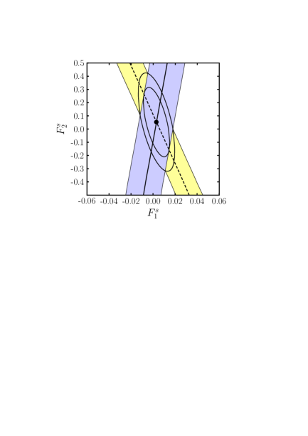
Figure 1: Results from [14] for the strange form factors at $t\simeq-0.1\,\,\operatorname{GeV}^{2}$. The dark (violet) band represents the result for $G_{E}^{s}$, and the light (yellow) band the one for $G_{E}^{s}+0.09\,G_{M}^{s}$. If one neglects the difference of the associated $t$ values one obtains the central value given in (14), which is shown as a bullet. Also shown are the corresponding $1\sigma$ and $2\sigma$ ellipses.

2.2 Unpolarized parton densities

The determination of parton densities (PDFs) from unpolarized hard scattering processes has made significant progress in the recent decade, in particular thanks to data with high precision and a large kinematical reach from HERA and from the Tevatron. The knowledge of strange distributions is much less advanced, because the observables that dominate global fits of parton densities have little sensitivity to $s$ or $\bar{s}$. This holds in particular for inclusive deep inelastic scattering (DIS) in kinematics where photon exchange is dominant. More specific constraints on $s$ and $\bar{s}$ distributions come from fixed-target DIS experiments with $\nu$ and $\bar{\nu}$ beams. Thanks to such measurements, there have recently been dedicated attempts to determine $s(x)$ and $\bar{s}(x)$ without strong assumptions on their relation with the light sea quark distributions $\bar{u}(x)$ and $\bar{d}(x)$.

In Table 2 we give the moments $\langle x(s+\bar{s})\mskip 1.5mu\rangle$ obtained in recent PDF extractions. The study in [21] was dedicated to strangeness and explored a number of fits at NLO in $\alpha_{s}$. The extractions in [22, 23] were performed at NNLO. The table also gives the moment $\langle x(\bar{u}+\bar{d})\mskip 1.5mu\rangle$, whose values range from $6.21\times 10^{-2}$ to $6.79\times 10^{-2}$ and thus show a much smaller spread than for $\langle x(s+\bar{s})\mskip 1.5mu\rangle$. The ratio of $\langle x(s+\bar{s})\mskip 1.5mu\rangle$ and $\langle x(\bar{u}+\bar{d})\mskip 1.5mu\rangle$ is between $0.36$ and $0.72$ and quantifies the suppression of strangeness in the light quark sea. We furthermore show the flavor asymmetry $\langle x(\bar{u}-\bar{d})\mskip 1.5mu\rangle$, which like $\langle x(s-\bar{s})\mskip 1.5mu\rangle$ is not generated by simple $g\to q\bar{q}$ splitting and hence requires more subtle dynamics in order to be nonzero. The ratio of $\langle x(\bar{u}-\bar{d})\mskip 1.5mu\rangle$ and $\langle x(\bar{u}+\bar{d})\mskip 1.5mu\rangle$ varies between $-7\%$ and $-14\%$. The parton densities corresponding to the entries in the table are plotted in Fig. 2. We note that there are no experimental constraints on $\bar{u}(x)-\bar{d}(x)$ at small $x$, so that the large difference between the results of [22] and [21, 23] for this combination of densities is a consequence of the different functional forms assumed in the fits.

	CTEQ6.5S [21]
set	$\phantom{-}0$	$\phantom{-}1$	$\phantom{-}2$	$\phantom{-}3$	$\phantom{-}4$	$-0$	$-1$	$-2$
$\langle x(s+\bar{s})\mskip 1.5mu\rangle$	$\phantom{-}3.35$	$\phantom{-}2.46$	$\phantom{-}4.44$	$\phantom{-}2.45$	$\phantom{-}4.30$	$\phantom{-}3.72$	$\phantom{-}3.48$	$\phantom{-}4.04$
$\langle x(\bar{u}+\bar{d})\mskip 1.5mu\rangle$	$\phantom{-}6.55$	$\phantom{-}6.79$	$\phantom{-}6.21$	$\phantom{-}6.74$	$\phantom{-}6.35$	$\phantom{-}6.54$	$\phantom{-}6.65$	$\phantom{-}6.37$
$\langle x(\bar{u}-\bar{d})\mskip 1.5mu\rangle$	$-0.72$	$-0.75$	$-0.69$	$-0.74$	$-0.69$	$-0.74$	$-0.76$	$-0.45$

Table 2: Results of different PDF fits for the moments $\langle x(s+\bar{s})\mskip 1.5mu\rangle$, $\langle x(\bar{u}+\bar{d})\mskip 1.5mu\rangle$ and $\langle x(\bar{u}-\bar{d})\mskip 1.5mu\rangle$. All numbers are given in units of $10^{-2}$ and refer to the scale $\mu=2\,\operatorname{GeV}$ in the $\overline{\mathrm{MS}}$ scheme.

	Alekhin 06 [22]	MRST 2006 [23]
$\langle x(s+\bar{s})\mskip 1.5mu\rangle$	$\phantom{-}3.40$	$\phantom{-}3.89$
$\langle x(\bar{u}+\bar{d})\mskip 1.5mu\rangle$	$\phantom{-}6.56$	$\phantom{-}6.77$
$\langle x(\bar{u}-\bar{d})\mskip 1.5mu\rangle$	$-0.56$	$-0.92$

\psfrag{xx}[c][c]{\small$x$}\psfrag{tt}[c][c]{\small$x(s+\bar{s})$}\psfrag{bb}[r][c]{\footnotesize CTEQ6.5S$0$}\psfrag{dd}[r][c]{\footnotesize Alekhin 06}\psfrag{hh}[r][c]{\footnotesize MRST 2006}\includegraphics[width=235.61981pt,bb=80 50 385 295]{Cteq6.5-s+sbar.eps}

\psfrag{xx}[c][c]{\small$x$}\psfrag{tt}[c][c]{\small$x(s+\bar{s})$}\psfrag{bb}[r][c]{\footnotesize CTEQ6.5S$0$}\psfrag{dd}[r][c]{\footnotesize Alekhin 06}\psfrag{hh}[r][c]{\footnotesize MRST 2006}\includegraphics[width=235.61981pt,bb=80 50 385 295]{comp-s+sbar.eps}

\psfrag{xx}[c][c]{\small$x$}\psfrag{tt}[c][c]{\small$x(s+\bar{s})$}\psfrag{bb}[r][c]{\footnotesize CTEQ6.5S$0$}\psfrag{dd}[r][c]{\footnotesize Alekhin 06}\psfrag{hh}[r][c]{\footnotesize MRST 2006}\psfrag{tt}[c][c]{\small$x(\bar{u}+\bar{d})$}\includegraphics[width=235.61981pt,bb=80 50 385 295]{Cteq6.5-ubar+dbar.eps}

\psfrag{xx}[c][c]{\small$x$}\psfrag{tt}[c][c]{\small$x(s+\bar{s})$}\psfrag{bb}[r][c]{\footnotesize CTEQ6.5S$0$}\psfrag{dd}[r][c]{\footnotesize Alekhin 06}\psfrag{hh}[r][c]{\footnotesize MRST 2006}\psfrag{tt}[c][c]{\small$x(\bar{u}+\bar{d})$}\includegraphics[width=235.61981pt,bb=80 50 385 295]{comp-ubar+dbar.eps}

\psfrag{xx}[c][c]{\small$x$}\psfrag{tt}[c][c]{\small$x(s+\bar{s})$}\psfrag{bb}[r][c]{\footnotesize CTEQ6.5S$0$}\psfrag{dd}[r][c]{\footnotesize Alekhin 06}\psfrag{hh}[r][c]{\footnotesize MRST 2006}\psfrag{tt}[c][c]{\small$x(\bar{u}+\bar{d})$}\psfrag{tt}[c][c]{\small$x(\bar{u}-\bar{d})$}\includegraphics[width=235.61981pt,bb=80 50 385 295]{Cteq6.5-ubar-dbar.eps}

\psfrag{xx}[c][c]{\small$x$}\psfrag{tt}[c][c]{\small$x(s+\bar{s})$}\psfrag{bb}[r][c]{\footnotesize CTEQ6.5S$0$}\psfrag{dd}[r][c]{\footnotesize Alekhin 06}\psfrag{hh}[r][c]{\footnotesize MRST 2006}\psfrag{tt}[c][c]{\small$x(\bar{u}+\bar{d})$}\psfrag{tt}[c][c]{\small$x(\bar{u}-\bar{d})$}\includegraphics[width=235.61981pt,bb=80 50 385 295]{comp-ubar-dbar.eps}

Figure 2: Different combinations of parton densities at $\mu=2\,\operatorname{GeV}$. Left: comparison of the different sets from CTEQ6.5S [21]. Right: comparison of set 0 from CTEQ6.5S [21] with Alekhin 06 [22] and MRST 2006 [23].

The CTEQ6.5S study [21] also performed fits where $s(x)$ and $\bar{s}(x)$ were allowed to be different. An essential input for constraining this difference are the CCFR and NuTeV data for dimuon production in $\nu$ and $\bar{\nu}$ DIS [24]. The parameterization in [21] was chosen such that $s(x)-\bar{s}(x)$ has precisely one zero crossing. The resulting momentum asymmetry at scale $\mu=2\,\operatorname{GeV}$ was found to be

$$\langle x(s-\bar{s})\mskip 1.5mu\rangle=\begin{cases}\phantom{-}2.0\phantom{0}\times 10^{-3}&\leavevmode\nobreak\ \leavevmode\nobreak\ (\text{set $-0$})\,,\\ -0.94\times 10^{-3}&\leavevmode\nobreak\ \leavevmode\nobreak\ (\text{set $-1$})\,,\\ \phantom{-}2.9\phantom{0}\times 10^{-3}&\leavevmode\nobreak\ \leavevmode\nobreak\ (\text{set $-2$})\,,\end{cases}$$ (16)

where set $-0$ corresponds to the best fit, whereas sets $-1$ and $-2$ were chosen to give the smallest and largest values of $\langle x(s-\bar{s})\mskip 1.5mu\rangle$, respectively. The ratio of $\langle x(s-\bar{s})\mskip 1.5mu\rangle$ and $\langle x(s+\bar{s})\mskip 1.5mu\rangle$ in the three fits has respective values $5.4\%$, $-2.7\%$ and $7.2\%$, which is somewhat smaller in size than the ratio of $\langle x(\bar{u}-\bar{d})\mskip 1.5mu\rangle$ and $\langle x(\bar{u}+\bar{d})\mskip 1.5mu\rangle$ in the non-strange sector. The left panel in Fig. 3 shows the asymmetry $s(x)-\bar{s}(x)$ obtained in these fits. We note that the best fit (set $-0$) is quite similar to preliminary results obtained by the MSTW collaboration [25]. It should be emphasized that a wider range of shapes is obtained if one allows for a variation of the small-$x$ behavior of $s(x)-\bar{s}(x)$, which is not well constrained by data. This is documented in a previous study by CTEQ [26] and shown in the right panel of Fig. 3.

\psfrag{xx}[c][c]{\small$x$}\psfrag{tt}[c][c]{\small$x(s-\bar{s})$}\psfrag{bb}[l][c]{\footnotesize set $-2$}\psfrag{bd}[l][c]{\footnotesize\phantom{set} $-0$}\psfrag{dd}[l][c]{\footnotesize\phantom{set} $-1$}\includegraphics[width=235.61981pt,bb=80 50 385 295]{Cteq6.5-s-sbar.eps}

\psfrag{xx}[c][c]{\small$x$}\psfrag{tt}[c][c]{\small$x(s-\bar{s})$}\psfrag{bb}[l][c]{\footnotesize set $-2$}\psfrag{bd}[l][c]{\footnotesize\phantom{set} $-0$}\psfrag{dd}[l][c]{\footnotesize\phantom{set} $-1$}\psfrag{bb}[l][c]{\footnotesize B$+$}\psfrag{bd}[l][c]{\footnotesize B}\psfrag{dd}[l][c]{\footnotesize B$-$}\psfrag{hh}[l][c]{\footnotesize C}\includegraphics[width=235.61981pt,bb=80 50 385 295]{Cteq6-s-sbar.eps}

Figure 3: The strangeness asymmetry distribution at scale $\mu=2\,\operatorname{GeV}$. The left panel shows the fits of the CTEQ6.5S analysis [21] and the right panel those of CTEQ6 [26]. Sets B and C correspond to different assumptions on the small-$x$ behavior of $s(x)-\bar{s}(x)$, whereas sets $-1$ and B$-$ ($-2$ and B$+$) have been chosen to minimize (maximize) the moment $\langle x(s-\bar{s})\mskip 1.5mu\rangle$.

2.3 Polarized parton densities

The polarization of strange quarks and antiquarks in the proton is not well known at present, for similar reasons as in the case of unpolarized parton densities. Many determinations of polarized PDFs in the literature, such as those in [27, 28, 29], are restricted to the structure functions for inclusive DIS with electron or muon beams, which does not permit a separate determination of strange densities. This is highlighted in the “valence” scenario of [27], which assumes $\Delta\bar{s}(x)=\Delta s(x)=0$ at the starting scale $\mu=0.63\,\operatorname{GeV}$ of evolution. This gives a tiny moment $\langle\Delta s+\Delta\bar{s}\mskip 1.5mu\rangle\approx-4\times 10^{-3}$ at $\mu=1\,\operatorname{GeV}$. The study in [30] additionally fits RHIC data for $\pi^{0}$ production, which has no particular sensitivity to strangeness either. A process that is specifically sensitive to strangeness is semi-inclusive kaon production in DIS, which has been measured by HERMES [31]. The study by de Florian et al. [32] includes these data and gives two sets of fits corresponding to different fragmentation functions. It does not assume flavor SU(3) symmetry in the polarized sea, allowing $\Delta\bar{s}(x)$ to differ from $\Delta\bar{u}(x)$ and $\Delta\bar{d}(x)$. We note that a recent analysis of semi-inclusive hadron production by COMPASS reported evidence that the polarized sea is not flavor symmetric and that $\langle\Delta\bar{u}\mskip 1.5mu\rangle$ and $\langle\Delta\bar{d}\mskip 1.5mu\rangle$ may have opposite sign [34]. All analyses performed so far assume $\Delta\bar{s}(x)=\Delta s(x)$.

In Table 3 we list the values obtained in recent analyses for the first moment $\langle\Delta s+\Delta\bar{s}\mskip 1.5mu\rangle$. Note that $1/2$ times this moment gives the contribution of strange quarks and antiquarks to the total spin $1/2$ of the nucleon. The values from the analyses [27, 28, 29, 30] have been obtained with parameterizations where the polarized sea quark densities are equal, $\Delta\bar{u}(x)=\Delta\bar{d}(x)=\Delta\bar{s}(x)$, so that they should not be regarded as specific determinations of the polarization of the strange sea. Rather, they indicate that the contribution of sea quarks to the nucleon spin is negative and of moderate magnitude. The different results of the study [32] illustrate that a flavor decomposition of this contribution is currently affected with considerable uncertainties. The numbers do not suggest that the strangeness contribution to the nucleon spin is very much suppressed compared with the light flavors $\bar{u}$ and $\bar{d}$, but further data and analyses are clearly necessary to settle this issue. As a further word of caution we remark that an important fraction of the moments in Table 3 comes from the region of small $x$, where the polarized densities are not constrained by data. Quantitative discussions are given in [31, 28].

	GRSV 2000 [27]	BB [28]		LSS 05 [29]		AAC 06 [30]
set	“standard”	3	4	1	2	1	2
$\langle\Delta s+\Delta\bar{s}\mskip 1.5mu\rangle=2\langle\Delta\bar{q}\mskip 1.5mu\rangle$	$-0.126$	$-0.148$	$-0.143$	$-0.122$	$-0.140$	$-0.10$	$-0.12$

Table 3: Lowest moments of polarized parton densities. All analyses shown set $\Delta s(x)=\Delta\bar{s}(x)$, and all except for [32] take $\Delta\bar{u}(x)=\Delta\bar{d}(x)=\Delta\bar{s}(x)$. The corresponding PDFs have been determined at NLO accuracy in the $\overline{\mathrm{MS}}$ scheme and refer to the scale $\mu=1\,\operatorname{GeV}$.

	DNS [32, 33]
set	KRE	KKP
$\langle\Delta s+\Delta\bar{s}\mskip 1.5mu\rangle$	$-0.095$	$-0.090$
$\langle\Delta\bar{u}\mskip 1.5mu\rangle$	$-0.046$	$\phantom{-}0.076$
$\langle\Delta\bar{d}\mskip 1.5mu\rangle$	$-0.048$	$-0.101$

3 Theoretical approaches

3.1 Electromagnetic form factors

The strangeness contributions to the electromagnetic and axial form factors of the nucleon have been studied in a large number of theoretical approaches (with many studies focusing on the strange magnetic moment or the electric charge radius) . Detailed reviews and discussions can be found in [35, 7, 36]. In Table 4 we list a small number of recent results for the strange Dirac form factor at $-t=0.1\,\operatorname{GeV}^{2}$. We find a substantial spread between these results and remark that several of them are outside the range $-0.009\leq F_{1}^{s}\leq 0.015$ obtained from the experimental values (14) and (15).

Table 4: Theoretical results for the strange Dirac form factor at $t_{0}=-0.1\,\operatorname{GeV}^{2}$. The numbers for Refs. [43, 44, 45, 46, 47] have been read off from graphs. The value in the last row has been obtained from $G_{E}^{s}(t_{0})$ in [49] and $G_{M}^{s}(0)$ in [48] using the approximation $G_{M}^{s}(t_{0})\approx G_{M}^{s}(0)$, which was also made in Fig. 2 of [16]. Taking into account that $|G_{M}^{s}(t_{0})|<|G_{M}^{s}(0)|$ would increase the value of $F_{1}^{s}(t_{0})$.

Approach	reference	$F_{1}^{s}\bigl{(}t=-0.1\,\operatorname{GeV}^{2}\bigr{)}$
Perturbative chiral quark model	[43]	$\phantom{-}0.003\phantom{(0)}$
Chiral quark soliton model ($\pi$)	[44]	$\phantom{-}0.063\phantom{(0)}$
Chiral quark soliton model ($K$)	[44]	$\phantom{-}0.028\phantom{(0)}$
Vector meson dominance	[45]	$-0.07\phantom{0(0)}$
Vector meson dominance	[46]	$\phantom{-}0.014\phantom{(0)}$
Lattice	[47]	$\phantom{-}0.015(5)$
Lattice $+$ measured magnetic moments and charge radii	[48, 49]	$\phantom{-}0.000(6)$

The calculation of strange form factors is challenging in many theoretical approaches. A large number of studies are based on the meson cloud picture, where the nucleon fluctuates into a $K$ and a $\Sigma$ or $\Lambda$. The coupling to the strangeness current then proceeds through valence degrees of freedom, namely the $\bar{s}$ in the kaon and the $s$ in the hyperon. Concerns have been raised about the quantitative reliability of such calculations, based on the possible importance of unitarity corrections [37] and of higher-mass states [38, 39] such as $K^{*}$ mesons [39]. There seems to be no consensus about these issues in the literature, see [40, 41] and [36]. We will not quantitatively use the meson cloud picture in the present work, but use it as a qualitative guide in Sect. 4.2. Chiral perturbation theory provides a systematic framework for calculations in terms of hadron degrees of freedom, but its predictive power for strange form factors is limited, as discussed in [42].

Kaons also play an essential role in chiral quark models such as the one in [43], where the nucleon is described in terms of three constituent quarks coupling to the pseudo-Goldstone bosons. In this approach, nonzero strange form factors are due to the splitting of a $u$ or $d$ quark into a kaon and an $s$ quark. The chiral quark soliton model [44] does not rely on the constituent quark picture, containing as degrees of freedom both quarks and antiquarks coupling to pions and kaons.

A different approach is based on dispersion relations, which represent the form factors for spacelike $t$ in terms of an integral over their imaginary parts in the timelike region. The assumption that the dispersion integral is dominated by single vector meson states leads to the vector meson dominance approximation, which underlies many calculations of the strange form factors. A typical procedure is to fix the relevant nucleon-meson coupling constants from the isoscalar electromagnetic form factors of the nucleon and then to predict the form factors of the strangeness current. Such analyses often obtain rather large couplings of the nucleon to the $\omega(782)$ and the $\phi(1020)$, see for instance [45]. These large couplings are in strong conflict with determinations from nucleon-nucleon potential studies [50, 51] or from dispersion relations for forward nucleon-nucleon scattering [52], with SU(6) symmetry [53], and in the case of the $\phi$ with the OZI rule. To understand why fits of nucleon form factors with a small number of vector meson resonances can give large couplings, we consider the simplified case of just two mesons with masses $m_{1}$ and $m_{2}$,

$$\frac{a_{1}}{m_{1}^{2}-t}+\frac{a_{2}}{m_{2}^{2}-t} =\frac{a_{1}(m_{2}^{2}-m_{1}^{2})-(a_{1}+a_{2})(t-m_{1}^{2})}{m_{1}^{2}\mskip 1.5mum_{2}^{2}-(m_{1}^{2}+m_{2}^{2})\,t+t^{2}}\,.$$ (17)

In order to obtain a $1/t^{2}$ behavior of the isoscalar form factor at large $-t$, one must have $a_{1}\approx-a_{2}$ to keep the term with $t$ in the numerator small. At $t=0$ the form factor is then approximately given by $a_{1}(m_{2}^{2}-m_{1}^{2})/(m_{1}^{2}\mskip 1.5mum_{2}^{2})$, and the small mass difference between $\phi(1020)$ and $\omega(782)$ forces the couplings $a_{1}$ and $a_{2}$ to be large. Taking into account higher-mass resonances significantly reduces this trend. As an illustration, we have fitted the isoscalar nucleon form factors to a sum of contributions from $\phi(1020)$, $\omega(782)$ and $\omega(1420)$, with or without an additional contribution from $\omega(1650)$. We require an asymptotic behavior $F_{1}^{p}+F_{1}^{n}\sim 1/t^{2}$ at large $-t$, which provides a linear relation between the different meson couplings in generalization of the simple case we just discussed. With the normalization condition $F_{1}^{p}(0)+F_{1}^{n}(0)=1$ this leaves two free parameters if the $\omega(1650)$ is included and a single parameter if this resonance is omitted. For the meson-nucleon couplings relevant to the Dirac form factors we obtain

$$g_{\phi NN}^{V} =-9.13\,, g_{\omega NN}^{V} =20.6$$ (18)

in the fit without $$\omega(1650) \smash{G^{V}_{NN\phi}} G^{V}_{NN\omega} \omega(1650)$$, where the couplings refer to the ground state mesons and are denoted by and in [51]. Including the , we obtain a good description of the data with

$$g_{\phi NN}^{V} =4.69\,, g_{\omega NN}^{V} =11.9\,,$$ (19)

where $g_{\omega NN}^{V}$ is fixed to a value as small as the data permits, in order to minimize the tension with the still lower values obtained in [50, 52, 53]. Taking both couplings as free fit parameters we find $g_{\phi NN}^{V}=-0.06$ and $g_{\omega NN}^{V}=14.9$. Similar values have been obtained in [54].

This simple exercise suggests to take with great care the corresponding predictions for strange form factors, where contributions from $\phi$ resonances are strongly enhanced compared with those from $\omega$ states. A more realistic treatment requires the inclusion of continuum states, as has for instance been done in [55, 56]. The analysis in [56] found that the inclusion of the $K\bar{K}$ and $\rho\pi$ continua makes the interpretation of a residual $\phi$ resonance contribution ambiguous.

3.2 The strangeness asymmetry $s(x)-\bar{s}(x)$

The meson cloud picture naturally induces an asymmetry in the momentum distribution of strange quarks and antiquarks, which was first observed in [57] and underlies many calculations [58, 59, 60, 61, 62, 63, 64]. In this picture, the densities of $s$ and $\bar{s}$ in the nucleon are given as convolutions of the longitudinal momentum distributions of the kaon or hyperon within the nucleon and the valence distribution of $\bar{s}$ in the kaon or of $s$ in the hyperon. A similar mechanism is realized in chiral quark models [65], where the constituent quarks of the proton can fluctuate into a kaon and a strange quark. There is a significant spread among meson cloud model predictions for the shape of $s(x)-\bar{s}(x)$, including its sign and the number of zero crossings, see e.g. the comparative study in [63]. The inclusion of $K^{*}$ fluctuations in [64] also had a significant effect, changing even the sign of the momentum asymmetry $\langle x(s-\bar{s})\mskip 1.5mu\rangle$ compared to the result with kaon fluctuations alone. We note that the predictions for $s-\bar{s}$ in such models typically have a zero at a value of $x$ much larger than $0.01$ and are thus rather different from the results obtained in the PDF fits [21, 25].

The study [66] pointed out that in perturbative evolution at three-loop accuracy and beyond, graphs with three-gluon exchange in the $t$-channel generate an $s-\bar{s}$ asymmetry. Starting with $s(x)=\bar{s}(x)$ at the low scale $\mu=0.51\,\operatorname{GeV}$, the authors of [66] find that $s(x)-\bar{s}(x)$ for $\mu\geq 2\,\operatorname{GeV}$ is positive at small and negative at intermediate to large $x$, with $\langle x(s-\bar{s})\rangle\approx-5\times 10^{-4}$. This is much smaller than the central fit results in [21, 25], which suggests that this perturbative mechanism plays only a minor role in the generation of the momentum asymmetry.

4 Relating the strange Dirac form factor to $s(x)-\bar{s}(x)$

We now formulate a model ansatz for the $C$ odd part of the generalized parton distribution $H^{s}$ at zero skewness, which will allow us to calculate the Dirac form factor $F_{1}^{s}$ from the phenomenologically extracted asymmetry $s-\bar{s}$ of momentum distributions. Following previous studies of generalized parton distributions in the non-strange sector [68, 5, 69, 70], we assume an exponential $t$ dependence with an $x$ dependent slope and set

$$H^{s}(x,t)-H^{\bar{s}}(x,t)=\bigl{[}s(x)-\bar{s}(x)\bigr{]}\,e^{\mskip 1.5mutf_{s}(x)}\,,$$ (20)

where for the slope we take the simple form

$$f_{s}(x)=\alpha^{\prime}(1-x)\log\frac{1}{x}\,,$$ (21)

which was already proposed in [5]. With (3) it is easy to see that the profile function $f_{s}(x)$ has a simple physical interpretation in terms of the average squared impact parameter

$$\langle b^{2}\rangle_{x} =\frac{\int d^{2}\boldsymbol{b}\;\boldsymbol{b}^{2}\bigl{[}s(x,b)-\bar{s}(x,b)\bigr{]}}{\int d^{2}\boldsymbol{b}\,\bigl{[}s(x,b)-\bar{s}(x,b)\bigr{]}}=4f_{s}(x)$$ (22)

associated with the difference between $s$ and $\bar{s}$ distributions. As shown in [71], a finite average transverse size of parton configurations with $x\to 1$ in the nucleon requires $\langle b^{2}\rangle_{x}$ to vanish at least like $(1-x)^{2}$ in this limit, which is obviously satisfied for the ansatz (21).

In the opposite limit $x\to 0$, we use simple Regge phenomenology as a guide for our parameterization. The form (21) corresponds to the behavior $H^{s}-H^{\bar{s}}\sim x^{-\alpha(t)}$, which arises from the exchange of a single Regge pole with a linear trajectory $\alpha(t)=\alpha(0)+\alpha^{\prime}t$, or from the superposition of several Regge poles with the same value of $\alpha^{\prime}$. This is a generalization to finite $t$ of a small-$x$ behavior $x^{-\alpha}$ for the usual parton densities, which is consistent with phenomenology. The leading Regge trajectory that can contribute to $H^{s}-H^{\bar{s}}$ is the one for the $\phi$ mesons, and assuming a linear form $\alpha_{\phi}(t)=\alpha_{\phi}(0)+\alpha^{\prime}t$ one obtains $\alpha_{\phi}(0)=0.13$ and $\alpha^{\prime}=0.84\,\operatorname{GeV}^{-2}$ from the masses and spins of $\phi(1020)$ and $\phi_{3}(1850)$. This value of $\alpha^{\prime}$ is close to the one for other meson trajectories, such as the ones for the $\rho$ and $\omega$. The $\phi$ trajectory contributes to soft hadronic scattering processes like kaon-nucleon scattering or photoproduction of the $\phi$ meson. It is however neglected in most analyses of these processes (which is justified if the $\phi\mskip 1.5mu$-nucleon coupling is sufficiently small, see our discussion in Sect. 3.1). An exception is the analysis of the total kaon-nucleon cross sections performed by Barger and Olsson [67], who found an intercept $\alpha_{\phi}(0)=0.33\pm 0.06$ of similar size as the result obtained from the hadronic spectrum. We emphasize that in our approach we do not need an explicit value for the $\phi\mskip 1.5mu$-nucleon coupling, since the normalization in (20) is fixed by the difference $s-\bar{s}$ of parton distributions.

We note that the CTEQ6.5S densities at $\mu=2\,\operatorname{GeV}$ are well approximated by

$$x(s-\bar{s})\approx ax^{0.28}$$ (23)

in the region $10^{-5}<x<10^{-4}$, with $a=-0.031,+0.023,-0.044$ for the respective sets $-0,-1,-2$. This corresponds to $\alpha(0)=0.72$, which is quite far from the values we estimate for the $\phi$ trajectory. There are however no experimental constraints for the behavior of $s-\bar{s}$ at very small $x$, and a value of $\alpha(0)$ between $0.1$ and $0.4$ is within the range for which a good description of all relevant data has been obtained in the CTEQ study [26].

Using an ansatz as in (20) for the valence combinations $H^{u}-H^{\bar{u}}$ and $H^{d}-H^{\bar{d}}$, we obtained in [69] a good description of the electromagnetic Dirac form factors of proton and neutron. Given the wealth of data in this case, we chose in that study more complicated forms than (21) for the profile functions $f_{u}(x)$ and $f_{d}(x)$. We find that for $10^{-4}<x<0.1$ they are both very well approximated by the form (21) with $\alpha^{\prime}=1\,\operatorname{GeV}^{-2}$, which remains close to $f_{u}(x)$ for $x>0.1$. Given the fast decrease of $s(x)-\bar{s}(x)$ with $x$, the small-$x$ region turns out to be most important for our calculation of $F_{1}^{s}$.

We take the ansatz (20) with the CTEQ6.5S densities [21] at $\mu=2\,\operatorname{GeV}$ as input, where the chosen scale is to be considered as a compromise between a small value appropriate for arguments based on hadronic Regge phenomenology and a large value where the densities are sufficiently constrained by experimental data. In the left panel of Fig. 4 we show the values of $F_{1}^{s}(t)$ obtained with the best fit (set $-0$) and with the alternative fits (sets $-1$ and $-2$). The central curves are for $\alpha^{\prime}=1\,\operatorname{GeV}^{-2}$ in (21), and the bands correspond to $\alpha^{\prime}$ between $0.85\,\operatorname{GeV}^{-2}$ and $1.15\,\operatorname{GeV}^{-2}$. We regard this variation as an estimate of the parametric uncertainty within our model, with the lower value corresponding to the estimate of the $\phi$ trajectory from the meson masses. In the following we refer to the result with $\alpha^{\prime}=1\,\operatorname{GeV}^{-2}$ and CTEQ6.5S set $-0$ as our default prediction.

\psfrag{xx}[c][c]{\small$-t\;[\,\operatorname{GeV}^{2}]$}\psfrag{tt}[c][c]{\small$F_{1}^{s}(t)$}\psfrag{bb}[r][c]{\footnotesize$-0.5\,F_{1}^{n}(t)$}\includegraphics[width=235.61981pt,bb=80 50 385 295]{F1s-Cteq6.5.eps}

\psfrag{xx}[c][c]{\small$-t\;[\,\operatorname{GeV}^{2}]$}\psfrag{tt}[c][c]{\small$F_{1}^{s}(t)$}\psfrag{bb}[r][c]{\footnotesize$-0.5\,F_{1}^{n}(t)$}\includegraphics[width=235.61981pt,bb=80 50 385 295]{F1s-Cteq6.eps}

Figure 4: The strange Dirac form factor obtained from the sum rule (4) with the model ansatz in (20) and (21). Central curves are for $\alpha^{\prime}=1\,\operatorname{GeV}^{-2}$ and bands for $0.85\,\operatorname{GeV}^{-2}<\alpha^{\prime}<1.15\,\operatorname{GeV}^{-2}$. The corresponding parton densities are (from top to bottom): CTEQ6.5S sets $-2$, $-0$, $-1$ in the left panel and CTEQ6 sets B$+$, B, C, B$-$ in the right panel. The data point is our estimate (14) of $F_{1}^{s}$, and the dotted curve corresponds to the parameterization of $F_{1}^{n}$ discussed in the text.

If instead of taking (21) we set $f_{s}(x)$ equal to the profile functions $f_{u}(x)$ or $f_{d}(s)$ obtained in [69], the form factor lies within the bands in the figure, except in the region where $|F_{1}^{s}(t)|$ has its maximum. In that region, the difference of $F_{1}^{s}(t)$ obtained with the different profile functions just mentioned is at most $5\%$. As a further alternative, we have made the ansatz (20) at scale $\mu=1.3\,\operatorname{GeV}$, which is the starting scale of the CTEQ parameterizations. Taking the profile function (21) with $\alpha^{\prime}=1\,\operatorname{GeV}^{-2}$, we again obtain values within the bands of Fig. 4, except for deviations of up to 5% around the maximum of $|F_{1}^{s}(t)|$. Clearly, the largest spread in predictions for $F_{1}^{s}(t)$ within our model is due to the different parton densities used as input. To further explore this, we have taken the parameterizations from the CTEQ6 study [26] at $\mu=2\,\operatorname{GeV}$, which provides a wider range of shapes as we have seen in Fig. 3. The resulting curves for $F_{1}^{s}(t)$ are shown in the right panel of Fig. 4. We recall that sets $-1$ and $-2$ in [21] and sets B$-$ and B$+$ in [26] were chosen to minimize or maximize the moment $\langle x(s-\bar{s})\mskip 1.5mu\rangle$. They are hence not preferred, although consistent with the data fitted in [21, 26].

\psfrag{xx}[c][c]{\small$-t\;[\,\operatorname{GeV}^{2}]$}\psfrag{tt}[c][c]{}\psfrag{bb}[r][c]{\footnotesize$F_{1}^{n}(t)$}\psfrag{dd}[r][c]{\footnotesize$-4.5\,F_{1}^{s}(3.5\,t)$}\includegraphics[width=235.61981pt,bb=80 50 385 295]{F1n.eps}

Figure 5: Data for the neutron Dirac form factor and fit from [69]. The dotted line corresponds to our default prediction for $F_{1}^{s}$, obtained with $\alpha^{\prime}=1\,\operatorname{GeV}^{2}$ and CTEQ6.5S set $-0$. The curve is rescaled such that its minimum coincides with the one of $F_{1}^{n}$.

We see that in all cases the form factor $F_{1}^{s}(t)$ is quite small and fully compatible with the estimates (14) and (15) extracted from experiment. We remark that for most of our curves, a linear behavior $F_{1}^{s}(t)\propto t$ as in (15) is not a good approximation for $-t$ much above $0.1\,\operatorname{GeV}^{2}$.

It is instructive to compare our results with another small nucleon form factor, namely the Dirac form factor $F_{1}^{n}(t)$ of the neutron. Figure 5 shows data together with the default fit from [69], which we already mentioned in connection with the profile functions $f_{u}(x)$ and $f_{d}(x)$. The same parameterization multiplied by $-0.5$ is shown as a dotted curve in Fig. 4. We recall at this point that

$$F_{1}^{n}(t)=\tfrac{2}{3}F_{1}^{d}(t)-\tfrac{1}{3}F_{1}^{u}(t)-\tfrac{1}{3}F_{1}^{s}(t)\,,$$ (24)

where the labels on the r.h.s. indicate the quark flavor contributions to the Dirac form factor $F_{1}^{p}$ of the proton. The fit in [69] neglected the strange contribution in $F_{1}^{n}$ and in $F_{1}^{p}$. We see in Fig. 4 that our estimates for $F_{1}^{s}$ are at most half as large in magnitude as $F_{1}^{n}$ for $-t=0.2\,\operatorname{GeV}^{2}$, so that at that point $-\frac{1}{3}F_{1}^{s}$ contributes at most $1/6$ to the neutron form factor. For higher $-t$ we find that $F_{1}^{s}(t)$ decreases faster than $F_{1}^{n}(t)$, which we will explain shortly. Only at small $t$ do we find a stronger influence of the strangeness contribution. If our estimate is correct, this is of relevance for the flavor analysis of the Dirac radius of the neutron, which in more familiar terms can be expressed through the electric radius and a contribution from the magnetic moment,

$$\langle r^{2}\rangle_{1}^{n} \;=\;6\,\frac{d}{dt}F_{1}^{n}(t)\biggl{|}_{t=0}\;=\;6\,\frac{d}{dt}G_{E}^{n}(t)\biggl{|}_{t=0}-\frac{3\mu_{n}}{2m_{n}^{2}}\;\approx\;\langle r^{2}\rangle_{E}^{n}+0.127\,\operatorname{fm}^{2}\,.$$ (25)

Concerning the proton form factor, we find that the values of $F_{1}^{s}(t)$ shown in Fig. 4 amount to at most $3\%$ of $F_{1}^{p}(t)$ at any $t$.

4.1 The shape of $F_{1}^{s}(t)$

Let us now discuss the general features of $F_{1}^{s}(t)$ that emerge with our model ansatz, where we have

$$F_{1}^{s}(t) =\int_{0}^{1}dx\,\bigl{[}s(x)-\bar{s}(x)\bigr{]}\,e^{\mskip 1.5mutf_{s}(x)}\,,$$ (26)

$$\frac{d}{dt}\mskip 1.5muF_{1}^{s}(t) =\int_{0}^{1}dx\,\bigl{[}s(x)-\bar{s}(x)\bigr{]}\mskip 1.5muf_{s}(x)\,e^{\mskip 1.5mutf_{s}(x)}\,.$$ (27)

For the neutron form factor the situation is slightly more complicated even if we neglect the strangeness contribution, since the fit in [69] required different profile functions for $u$ and $d$ quarks. Since their difference is only moderate, the discussion of $F_{1}^{n}(t)$ is however quite similar.

With $f_{s}(x)$ being a decreasing function, the factor $e^{\mskip 1.5mutf_{s}(x)}$ increasingly suppresses small $x$ values in the integral (26) when $-t$ becomes larger. For increasing $-t$ the form factor $F_{1}^{s}$ is therefore connected with $s-\bar{s}$ at increasing values of $x$. With the profile function (21) we obtain the Drell-Yan relation $p={\textstyle\frac{1}{2}}(1+\beta)$ between the powers describing the asymptotic power laws $F_{1}^{s}\sim(-t)^{-p}$ for $t\to-\infty$ and $s-\bar{s}\sim(1-x)^{\beta}$ for $x\to 1$ [71, 69]. The difference $s-\bar{s}$ of sea quark distributions falls off faster with $x$ than the valence distributions $u-\bar{u}$ and $d-\bar{d}$, which are relevant for $F_{1}^{n}$, so that one generally expects $|F_{1}^{s}(t)|$ to decrease faster than $|F_{1}^{n}(t)|$ with $-t$. As Figs. 4 and 5 show, this is indeed the case in our model.

In Fig. 6 we show the integrands of $F_{1}^{s}$ and $dF_{1}^{s}/dt$ in (26) and (27). The integrands are multiplied with $x$ in the plots, so that with the logarithmic scale for $x$ we obtain the form factor or its derivative as the area under the corresponding curve. For $t=0$ the integrand of $F_{1}^{s}$ is $s(x)-\bar{s}(x)$, which gives a zero integral because of quantum number constraints. The integrand for the derivative $dF_{1}^{s}/dt$ has an extra factor $f_{s}(x)$, which enhances small $x$ values relative to larger ones. At $t=0$ one therefore has $dF_{1}^{s}/dt<0$ at $t=0$ if $s-\bar{s}$ is negative at small $x$ and positive at large $x$. This is the case for the CTEQ fits [21, 26] except for sets $-1$ and B$-$. As $-t$ increases, the factor $e^{\mskip 1.5mutf_{s}(x)}$ suppresses small $x$ values in (27), and for sufficiently large $-t$ the derivative $dF_{1}^{s}/dt$ has the opposite sign than at $t=0$. For some $t$ one hence obtains a maximum or minimum of $F_{1}^{s}(t)$. The value of $-t$ where this happens is larger for parameterizations of $s-\bar{s}$ which have the zero crossing at larger $x$, as one can check by comparing Figs. 3 and 4.

\psfrag{xx}[c][c]{\small$x$}\psfrag{tt}[c][c]{\small$x\mskip 1.5mu(H^{s}-H^{\bar{s}})$}\psfrag{bb}[l][c]{\footnotesize$t=0$}\psfrag{dd}[l][c]{\footnotesize$\phantom{t}=-0.2\,\operatorname{GeV}^{2}$}\psfrag{hh}[l][c]{\footnotesize$\phantom{t}=-0.5\,\operatorname{GeV}^{2}$}\includegraphics[width=230.80661pt,bb=80 50 385 295]{int-F1s.eps}

\psfrag{xx}[c][c]{\small$x$}\psfrag{tt}[c][c]{\small$x\mskip 1.5mu(H^{s}-H^{\bar{s}})$}\psfrag{bb}[l][c]{\footnotesize$t=0$}\psfrag{dd}[l][c]{\footnotesize$\phantom{t}=-0.2\,\operatorname{GeV}^{2}$}\psfrag{hh}[l][c]{\footnotesize$\phantom{t}=-0.5\,\operatorname{GeV}^{2}$}\psfrag{tt}[c][c]{\small$x\mskip 1.5mu\frac{d}{dt}(H^{s}-H^{\bar{s}})$}\includegraphics[width=230.80661pt,bb=80 50 385 295]{int-dF1s-dt.eps}

\psfrag{xx}[c][c]{\small$x$}\psfrag{tt}[c][c]{\small$x\mskip 1.5mu(H^{s}-H^{\bar{s}})$}\psfrag{bb}[l][c]{\footnotesize$t=0$}\psfrag{dd}[l][c]{\footnotesize$\phantom{t}=-0.2\,\operatorname{GeV}^{2}$}\psfrag{hh}[l][c]{\footnotesize$\phantom{t}=-0.5\,\operatorname{GeV}^{2}$}\psfrag{tt}[c][c]{\small$x\mskip 1.5mu\frac{d}{dt}(H^{s}-H^{\bar{s}})$}\psfrag{tt}[c][c]{\small$\frac{2}{3}x\mskip 1.5mu(H^{d}-H^{\bar{d}}\mskip 1.5mu)-\frac{1}{3}x\mskip 1.5mu(H^{u}-H^{\bar{u}})$}\psfrag{dd}[l][c]{\footnotesize$\phantom{t}=-0.7\,\operatorname{GeV}^{2}$}\psfrag{hh}[l][c]{\footnotesize$\phantom{t}=-1.4\,\operatorname{GeV}^{2}$}\includegraphics[width=230.80661pt,bb=80 50 385 295]{int-F1n.eps}

\psfrag{xx}[c][c]{\small$x$}\psfrag{tt}[c][c]{\small$x\mskip 1.5mu(H^{s}-H^{\bar{s}})$}\psfrag{bb}[l][c]{\footnotesize$t=0$}\psfrag{dd}[l][c]{\footnotesize$\phantom{t}=-0.2\,\operatorname{GeV}^{2}$}\psfrag{hh}[l][c]{\footnotesize$\phantom{t}=-0.5\,\operatorname{GeV}^{2}$}\psfrag{tt}[c][c]{\small$x\mskip 1.5mu\frac{d}{dt}(H^{s}-H^{\bar{s}})$}\psfrag{tt}[c][c]{\small$\frac{2}{3}x\mskip 1.5mu(H^{d}-H^{\bar{d}}\mskip 1.5mu)-\frac{1}{3}x\mskip 1.5mu(H^{u}-H^{\bar{u}})$}\psfrag{dd}[l][c]{\footnotesize$\phantom{t}=-0.7\,\operatorname{GeV}^{2}$}\psfrag{hh}[l][c]{\footnotesize$\phantom{t}=-1.4\,\operatorname{GeV}^{2}$}\psfrag{tt}[c][c]{\small$\frac{2}{3}x\mskip 1.5mu\frac{d}{dt}(H^{d}-H^{\bar{d}}\mskip 1.5mu)-\frac{1}{3}x\mskip 1.5mu\frac{d}{dt}(H^{u}-H^{\bar{u}})$}\includegraphics[width=230.80661pt,bb=80 50 385 295]{int-dF1n-dt.eps}

Figure 6: Upper plots: the scaled integrands of $F_{1}^{s}(t)$ and $dF_{1}^{s}(t)/dt$ in (26) and (27), obtained with our default prediction. Lower plots: the corresponding scaled integrands for $F_{1}^{n}(t)$ and $dF_{1}^{n}(t)/dt$, obtained with the default fit in [69]. The values of $t$ in the right panels are as for the corresponding curves on the left.

Figure 6 also shows the integrands for $F_{1}^{n}$ and $dF_{1}^{n}/dt$ for the default fit in [69]. The discussion for the sign of the derivative $dF_{1}^{n}/dt$ and the presence of a minimum of $F_{1}^{n}(t)$ proceeds in analogy to the case of the strangeness form factor. Since the zero crossing of $\frac{2}{3}(d-\bar{d})-\frac{1}{3}(u-\bar{u})$ occurs at much larger $x$ than the one of $s-\bar{s}$ in the CTEQ6.5S parameterizations, whereas the respective profile functions are similar, $|F_{1}^{n}(t)|$ assumes its maximum at significantly larger $-t$ than $|F_{1}^{s}(t)|$.

Let us at this point mention the PDFs extracted in [72]. In contrast to the analyses by CTEQ [21, 26] and MSTW [25], the strangeness asymmetry $x(s-\bar{s})$ in [72] has a zero at $0.4\raisebox{-3.0pt}{$\,\stackrel{{\scriptstyle\textstyle<}}{{\scriptstyle\sim}}$\,}x\raisebox{-3.0pt}{$\,\stackrel{{\scriptstyle\textstyle<}}{{\scriptstyle\sim}}$\,}0.5$ and a maximum at $x\sim 0.7$. Taking this distribution with the same profile functions $f_{s}(x)$ explored above, we obtain a form factor $F_{1}^{s}(t)$ with a very flat maximum $F_{1}^{s}\sim 0.0025$ for $1\,\operatorname{GeV}^{2}\raisebox{-3.0pt}{$\,\stackrel{{\scriptstyle\textstyle<}}{{\scriptstyle\sim}}$\,}-t\;\raisebox{-3.0pt}{$\,\stackrel{{\scriptstyle\textstyle<}}{{\scriptstyle\sim}}$\,}\;2\,\operatorname{GeV}^{2}$ and a slow decrease with $-t$. In this case, the bulk of the form factor integral (26) comes from very large $x$, where we deem our model for the profile function $f_{s}(x)$ associated with sea quarks very insecure. Since the study [72] used inclusive cross sections for $\nu$ and $\bar{\nu}$ DIS but no dimuon production data to constrain $s-\bar{s}$, we do not regard such a scenario as strongly motivated. This example illustrates however that within our model framework, strong changes in $s-\bar{s}$ result in qualitatively different forms of $F_{1}^{s}(t)$, which may eventually be ruled out by data.

The relations between the $x$ dependence of $s-\bar{s}$ and the $t$ dependence of $F_{1}^{s}(t)$ discussed in this subsection follow from the general features of our ansatz in (20) and (21) and will also hold for more complicated forms. The neutron form factor $F_{1}^{n}(t)$ and the combination $\frac{2}{3}(d-\bar{d})-\frac{1}{3}(u-\bar{u})$ of valence distributions, which are both much better known than their strangeness counterparts, provide an example where these relations are indeed seen and corroborate our prediction for the behavior of $F_{1}^{s}(t)$ with a given form of $s(x)-\bar{s}(x)$.

4.2 A modified ansatz

Our ansatz in (20) is special in that it assumes a $t$ dependence in the form of a global factor multiplying $s(x)-\bar{s}(x)$. It implies that the difference $s(x,b)-\bar{s}(x,b)$ of impact parameter densities has a Gaussian shape in $b$ and in particular does not change sign for given $x$. One may wonder whether this ansatz is too restrictive. The physical picture of meson cloud models for instance suggests that the typical transverse position of $s$ is smaller than for $\bar{s}$, since the $\bar{s}$ originates from a kaon, which due to its smaller mass tends to be at larger distances than the hyperon containing the $s$. If this effect is strong enough, one may have a node of $s(x,b)-\bar{s}(x,b)$ in $b$.

It is however important to realize that at $\mu=2\,\operatorname{GeV}$, where we formulate our model, the individual distributions of $s$ and $\bar{s}$ are not valence-like as they would be in a model valid at low resolution scale. For sets $-0$, $-1$ and $-2$ of the CTEQ6.5S parameterization at $\mu=2\,\operatorname{GeV}$ we find

$$x(s+\bar{s})\approx 0.2\,x^{-0.2}$$ (28)

in the region $10^{-5}<x<10^{-4}$, which is to be compared with (23). For $x<10^{-2}$ the ratio $(s-\bar{s})/(s+\bar{s})$ does not exceed $1\%$ in absolute size. It is natural to assume that the bulk of $s$ and $\bar{s}$ in that region is generated through gluon splitting $g\to s\bar{s}$ as described by perturbative evolution. This mechanism does not introduce an asymmetry in the transverse distribution of $s$ and $\bar{s}$. When introducing a more general ansatz for $H^{s}-H^{\bar{s}}$ than (20) we should hence make sure that the strong cancellation between $s$ and $\bar{s}$ at small $x$ takes place not only in the forward limit but also at nonzero $t$. With this in mind, we explore a variant of (20), given by

$$H^{s}(x,t)-H^{\bar{s}}(x,t)=s(x)\,e^{\mskip 1.5mutf_{s}(x)}-\bar{s}(x)\,e^{\mskip 1.5mut\bar{f}_{s}(x)}$$ (29)

with

$$f_{s}(x) =\alpha^{\prime}(1-x)\log\frac{1}{x}+A\mskip 1.5mux(1-x)^{2}\,,$$

$$\bar{f}_{s}(x) =\alpha^{\prime}(1-x)\log\frac{1}{x}+\bar{A}\mskip 1.5mux(1-x)^{2}\,,$$ (30)

where the prefactor $x$ in front of $A$ and $\bar{A}$ guarantees the cancellation just discussed, as long as $-tA$ and $-t\bar{A}$ are not too large. In the following we take values $2\,\operatorname{GeV}^{-2}$ and $4\,\operatorname{GeV}^{-2}$ for either $A$ or $\bar{A}$. With $\alpha^{\prime}=1\,\operatorname{GeV}^{-2}$ this respectively corresponds to a change of $f_{s}(x)$ or $\bar{f}_{s}(x)$ by a factor $1.2$ and $1.4$ at $x=0.2$, which one may view as a typical momentum fraction for $s$ and $\bar{s}$ in a model at low scale, where nonperturbative effects could generate an asymmetric distribution in impact parameter. In the left panel of Fig. 7 we show the corresponding impact parameter densities $s(x,b)-\bar{s}(x,b)$ and see that they indeed have nodes in $b$ when $A$ or $\bar{A}$ is equal to $4\,\operatorname{GeV}^{-2}$.

\psfrag{xx}[c][c]{\small$b\,[\,\operatorname{fm}]$}\psfrag{tt}[c][c]{\small$2\pi b\bigl{[}s(x,b)-\bar{s}(x,b)\bigr{]}$ \leavevmode\nobreak\ in\leavevmode\nobreak\ fm${}^{-1}$}\psfrag{bb}[r][c]{\footnotesize$A=0\quad\bar{A}=4$}\psfrag{dd}[r][c]{\footnotesize$\phantom{A}=0\quad\phantom{A}=0$}\psfrag{hh}[r][c]{\footnotesize$\phantom{A}=4\quad\phantom{A}=0$}\includegraphics[width=235.61981pt,bb=80 50 385 295]{impact-alt.eps}

\psfrag{xx}[c][c]{\small$b\,[\,\operatorname{fm}]$}\psfrag{tt}[c][c]{\small$2\pi b\bigl{[}s(x,b)-\bar{s}(x,b)\bigr{]}$ \leavevmode\nobreak\ in\leavevmode\nobreak\ fm${}^{-1}$}\psfrag{bb}[r][c]{\footnotesize$A=0\quad\bar{A}=4$}\psfrag{dd}[r][c]{\footnotesize$\phantom{A}=0\quad\phantom{A}=0$}\psfrag{hh}[r][c]{\footnotesize$\phantom{A}=4\quad\phantom{A}=0$}\psfrag{xx}[c][c]{\small$x$}\psfrag{tt}[c][c]{\small$x\mskip 1.5mu(H^{s}-H^{\bar{s}})$}\psfrag{bb}[l][c]{\footnotesize$A=0\quad\bar{A}=4$}\psfrag{dd}[l][c]{\footnotesize$\phantom{A}=0\quad\phantom{A}=0$}\psfrag{hh}[l][c]{\footnotesize$\phantom{A}=4\quad\phantom{A}=0$}\includegraphics[width=235.61981pt,bb=80 50 385 295]{int-alt.eps}

Figure 7: Left: the difference in the impact parameter distributions for strange quarks and antiquarks at $x=0.2$. The distributions are multiplied with $2\pi b$, so that the area under each curve gives $s(x)-\bar{s}(x)$. Right: the integrand (26) of the strange Dirac form factor at $-t=0.5\,\operatorname{GeV}^{2}$. The curves are for the ansatz in (29) and (4.2) with $\alpha^{\prime}=1\,\operatorname{GeV}^{-2}$ and different values of $A$ and $\bar{A}$ (given in units of $\,\operatorname{GeV}^{-2}$). For the parton densities we take CTEQ6.5S set $-0$ at $\mu=2\,\operatorname{GeV}$.

\psfrag{xx}[c][c]{\small$-t\;[\,\operatorname{GeV}^{2}]$}\psfrag{tt}[c][c]{\small$F_{1}^{s}(t)$}\psfrag{bb}[r][c]{\footnotesize$A=0\quad\bar{A}=4$}\psfrag{bd}[r][c]{\footnotesize$\phantom{A}=0\quad\phantom{A}=2$}\psfrag{dd}[r][c]{\footnotesize$\phantom{A}=0\quad\phantom{A}=0$}\psfrag{dh}[r][c]{\footnotesize$\phantom{A}=2\quad\phantom{A}=0$}\psfrag{hh}[r][c]{\footnotesize$\phantom{A}=4\quad\phantom{A}=0$}\includegraphics[width=235.61981pt,bb=80 50 385 295]{F1s-alt.eps}

Figure 8: The strange form factor obtained with the ansatz specified in Fig. 7. The curve for $A=\bar{A}=0$ corresponds to our default prediction in the previous subsections.

The form factors obtained with this ansatz are shown in Fig. 8. For $\bar{A}>0$, where $\bar{s}$ is concentrated at larger impact parameters than $s$, we find that $F_{1}^{s}$ is increased in size but not much changed in shape compared with our default prediction with $A=\bar{A}=0$. In contrast, we find that for sufficiently large $A>0$ the form factor $F_{1}^{s}$ changes sign at some finite $-t$. We can understand this at the level of the form factor integrand: for $f_{s}(x)>\bar{f}_{s}(x)$ the exponential factors in (29) give a stronger suppression in the first term, so that at large enough $x$ and $-t$ one can have $H^{s}(x,t)<H^{s}(x,t)$ despite $s(x)>\bar{s}(x)$. This is illustrated in the right panel of Fig. 7.

As discussed above, the meson cloud picture suggests that $s$ has smaller rather than larger typical impact parameters than $\bar{s}$, so that we do not see a particular physics motivation for our examples with $A>0$. However, they show that certain nontrivial correlations between the $x$ and $b$ dependence of the $s$ and $\bar{s}$ distributions can have quite drastic effects on $F_{1}^{s}(t)$, which may be observable in experiments with sufficient sensitivity and kinematic coverage.

4.3 Other form factors

With our model (20) for $H^{s}-H^{\bar{s}}$ we can also evaluate the Mellin moment $A_{3,0}^{s}(t)=\int_{-1}^{1}dx\,x^{2}H^{s}(x,t)$, which is a form factor of an operator with two covariant derivatives between the strange quark field and its conjugate. The factor $x^{2}$ strongly suppresses small $x$ values, and with the CTEQ parameterizations for $s-\bar{s}$ the integral is dominated by an $x$ region where the integrand has a definite sign. As a consequence $|A_{3,0}^{s}(t)|$ decreases monotonically with $-t$. Its value at $t=0$ is tiny, ranging from $-10^{-4}$ to $4\times 10^{-4}$ for the CTEQ6 and CTEQ6.5S parameterizations at $\mu=2\,\operatorname{GeV}$. Exceptions are the values $-6\times 10^{-4}$ and $10^{-3}$ for CTEQ6B$-$ and CTEQ6B$+$, respectively.

We do not attempt here to model the strangeness contributions to the energy-momentum and axial form factors, $A_{2,0}^{s}(t)$ and $F_{A}^{s}(t)$, which according to (9) and (10) are respectively related to $s+\bar{s}$ and $\Delta s+\Delta\bar{s}$. These distributions mix with gluons under evolution, which invalidates simple ansätze based on Regge trajectories for their small-$x$ behavior. This also holds at finite $t$ [73]. Since even the $t$ dependence of $H^{u}+H^{\bar{u}}$ and $H^{d}+H^{\bar{d}}$ is barely constrained at present, we see no clear guidance for how to model profile functions of $H^{s}+H^{\bar{s}}$ and $\widetilde{H}^{s}+\widetilde{H}^{\bar{s}}$. We expect however that these distributions have no zeroes in $x$, which certainly holds for their values at $t=0$ according to current PDF parameterizations. We therefore predict the corresponding form factors to decrease monotonically in absolute size, with values at $t=0$ given by the moments in Tables 2 and 3.

5 Summary

We have discussed several measures of strangeness in the nucleon. Strange quarks and antiquarks are not particularly rare in the proton: their contribution $\langle x(s+\bar{s})\mskip 1.5mu\rangle$ to the nucleon momentum is only suppressed by about a half compared with the one from light flavor antiquarks, $\langle x(\bar{u}+\bar{d})\mskip 1.5mu\rangle$. Their contribution $\langle\Delta s+\Delta\bar{s}\mskip 1.5mu\rangle$ to the spin of the proton is not well determined at present, but there are no indications that it is very much suppressed compared with $\langle\Delta\bar{u}+\Delta\bar{d}\mskip 1.5mu\rangle$.

More subtle quantities are asymmetries between strange quarks and antiquarks, most notably the asymmetry between the parton densities $s(x)$ and $\bar{s}(x)$, and the strange Dirac and Pauli form factors $F_{1}^{s}(t)$ and $F_{2}^{s}(t)$. A two dimensional Fourier transform of $F_{1}^{s}(t)$ yields the difference of spatial distributions for $s$ and $\bar{s}$ in the transverse plane, whereas $s(x)-\bar{s}(x)$ gives the difference of their distribution in longitudinal momentum. The two asymmetries are connected via generalized parton distributions at zero skewness, for which we have made a model ansatz in order to explore this connection quantitatively. Using as an input different sets of $s-\bar{s}$ distributions extracted by the CTEQ Collaboration, we find values of $F_{1}^{s}\bigl{(}t\simeq-0.1\,\operatorname{GeV}^{2}\bigr{)}$ between $-0.006$ and $0.012$, in good agreement with current experimental constraints. Many theoretical analyses of the electromagnetic nucleon form factors neglect the strangeness contributions. With our estimates this is at most a $3\%$ effect for $F_{1}^{p}(t)$. However, $|F_{1}^{s}(t)|$ might amount to as much as $1/6$ of $F_{1}^{n}(t)$ at $-t=0.2\,\operatorname{GeV}^{2}$. For higher $-t$ the relative contribution quickly decreases, whereas for lower $-t$ it may even be larger.

The general features of our model ansatz for generalized parton distributions lead to correlations between the $x$ dependence of $s-\bar{s}$ and the shape of $F_{1}^{s}(t)$. The best fits in the PDF extractions [21, 25, 26] yield forms where $s-\bar{s}$ is negative for small $x$ and positive for large $x$. With our ansatz, this gives a negative derivative $dF_{1}^{s}(t)/dt$ at $t=0$ and a maximum of the form factor at some value of $-t$. With a zero crossing of $s-\bar{s}$ at $x$ between $10^{-2}$ and $10^{-1}$, we find this maximum at $-t$ between $0.2\,\operatorname{GeV}^{2}$ and $0.4\,\operatorname{GeV}^{2}$. Analogous correlations are seen to hold between the combination $\frac{2}{3}(d-\bar{d})-\frac{1}{3}(u-\bar{u})$ of valence quark distributions and the neutron form factor $F_{1}^{n}(t)$, which we take as support for our predictions. Finally, a rapid decrease of $s-\bar{s}$ with $x$ reflects itself in a faster decrease of $F_{1}^{s}(t)$ compared with $F_{1}^{n}(t)$ for large $-t$. It will be interesting to confront these predictions with future data from parity violating electron-nucleon scattering.

References

- [1] S. Davidson, S. Forte, P. Gambino, N. Rius and A. Strumia, JHEP 0202 (2002) 037 [hep-ph/0112302].
- [2] M. E. Sainio, N Newslett. 16 (2002) 138 [hep-ph/0110413].
- [3] M. Diehl, Phys. Rept. 388 (2003) 41 [hep-ph/0307382].
- [4] A. V. Belitsky and A. V. Radyushkin, Phys. Rept. 418 (2005) 1 [hep-ph/0504030].
- [5] M. Burkardt, Int. J. Mod. Phys. A 18 (2003) 173 [hep-ph/0207047].
- [6] M. Burkardt, Phys. Lett. B 582 (2004) 151 [hep-ph/0309116].
- [7] D. T. Spayde et al. [SAMPLE Collaboration], Phys. Lett. B 583 (2004) 79 [nucl-ex/0312016].
- [8] F. E. Maas et al. [A4 Collaboration], Phys. Rev. Lett. 93 (2004) 022002 [nucl-ex/0401019].
- [9] K. A. Aniol et al. [HAPPEX Collaboration], Phys. Rev. C 69 (2004) 065501 [nucl-ex/0402004].
- [10] F. E. Maas et al. [A4 Collaboration], Phys. Rev. Lett. 94 (2005) 152001 [nucl-ex/0412030].
- [11] K. A. Aniol et al. [HAPPEX Collaboration], Phys. Rev. Lett. 96 (2006) 022003 [nucl-ex/0506010].
- [12] K. A. Aniol et al. [HAPPEX Collaboration], Phys. Lett. B 635 (2006) 275 [nucl-ex/0506011].
- [13] D. S. Armstrong et al. [G0 Collaboration], Phys. Rev. Lett. 95 (2005) 092001 [nucl-ex/0506021].
- [14] A. Acha et al. [HAPPEX collaboration], Phys. Rev. Lett. 98 (2007) 032301 [nucl-ex/0609002].
- [15] R. D. Young, J. Roche, R. D. Carlini and A. W. Thomas, Phys. Rev. Lett. 97 (2006) 102002 [nucl-ex/0604010].
- [16] R. D. Young, R. D. Carlini, A. W. Thomas and J. Roche, Phys. Rev. Lett. 99 (2007) 122003, arXiv:0704.2618 [hep-ph].
- [17] A. W. Thomas and R. D. Young, private communication.
- [18] A. V. Afanasev and C. E. Carlson, Phys. Rev. Lett. 94 (2005) 212301 [hep-ph/0502128].
- [19] H. Q. Zhou, C. W. Kao and S. N. Yang, Phys. Rev. Lett. 99 (2007) 262001, arXiv:0708.4297 [hep-ph].
- [20] J. A. Tjon and W. Melnitchouk, arXiv:0711.0143 [nucl-th].
- [21] H. L. Lai, P. Nadolsky, J. Pumplin, D. Stump, W. K. Tung and C. P. Yuan, JHEP 0704 (2007) 089 [hep-ph/0702268].
- [22] S. Alekhin, K. Melnikov and F. Petriello, Phys. Rev. D 74 (2006) 054033 [hep-ph/0606237].
- [23] A. D. Martin, W. J. Stirling, R. S. Thorne and G. Watt, Phys. Lett. B 652 (2007) 292 [arXiv:0706.0459 [hep-ph]].
- [24] M. Goncharov et al. [NuTeV Collaboration], Phys. Rev. D 64 (2001) 112006 [hep-ex/0102049].
- [25] R. Thorne, An update of the parton distributions for the LHC, DESY Colloquium, October 2007, http://indico.cern.ch/conferenceDisplay.py?confId=20453
- [26] F. Olness et al., Eur. Phys. J. C 40 (2005) 145 [hep-ph/0312323].
- [27] M. Glück, E. Reya, M. Stratmann and W. Vogelsang, Phys. Rev. D 63 (2001) 094005 [hep-ph/0011215].
- [28] J. Blümlein and H. Böttcher, Nucl. Phys. B 636 (2002) 225 [hep-ph/0203155].
- [29] E. Leader, A. V. Sidorov and D. B. Stamenov, Phys. Rev. D 73 (2006) 034023 [hep-ph/0512114].
- [30] M. Hirai, S. Kumano and N. Saito, Phys. Rev. D 74 (2006) 014015 [hep-ph/0603213].
- [31] A. Airapetian et al. [HERMES Collaboration], Phys. Rev. D 71 (2005) 012003 [hep-ex/0407032].
- [32] D. de Florian, G. A. Navarro and R. Sassot, Phys. Rev. D 71 (2005) 094018 [hep-ph/0504155].
- [33] R. Sassot, private communication.
- [34] M. Alekseev et al. [COMPASS Collaboration], arXiv:0707.4077 [hep-ex].
- [35] D. H. Beck and B. R. Holstein, Int. J. Mod. Phys. E 10 (2001) 1 [hep-ph/0102053].
- [36] M. J. Ramsey-Musolf, Eur. Phys. J. A 24S2 (2005) 197 [nucl-th/0501023].
- [37] M. J. Musolf, H. W. Hammer and D. Drechsel, Phys. Rev. D 55 (1997) 2741, Erratum ibid. D 62 (2000) 079901 [hep-ph/9610402].
- [38] P. Geiger and N. Isgur, Phys. Rev. D 55 (1997) 299 [hep-ph/9610445].
- [39] L. L. Barz et al., Nucl. Phys. A 640 (1998) 259 [hep-ph/9803221].
- [40] W. Melnitchouk and M. Malheiro, Phys. Lett. B 451 (1999) 224 [hep-ph/9901321].
- [41] H. Forkel, F. S. Navarra and M. Nielsen, Phys. Rev. C 61 (2000) 055206 [hep-ph/9904496].
- [42] B. Kubis, Eur. Phys. J. A 24S2 (2005) 97 [nucl-th/0504004].
- [43] V. E. Lyubovitskij, P. Wang, T. Gutsche and A. Faessler, Phys. Rev. C 66 (2002) 055204 [hep-ph/0207225].
- [44] A. Silva, H. C. Kim and K. Goeke, Phys. Rev. D 65 (2001) 014016, Erratum ibid. D 66 (2002) 039902 [hep-ph/0107185].
- [45] H. W. Hammer, U. G. Meissner and D. Drechsel, Phys. Lett. B 367 (1996) 323 [hep-ph/9509393].
- [46] S. Dubnička and A. Z. Dubničková, hep-ph/0608342.
- [47] R. Lewis, W. Wilcox and R. M. Woloshyn, Phys. Rev. D 67 (2003) 013003 [hep-ph/0210064].
- [48] D. B. Leinweber et al., Phys. Rev. Lett. 94 (2005) 212001 [hep-lat/0406002].
- [49] D. B. Leinweber et al., Phys. Rev. Lett. 97 (2006) 022001 [hep-lat/0601025].
- [50] M. M. Nagels, T. A. Rijken and J. J. De Swart, in: Few Body Systems and Nuclear Forces I, Procs. Graz 1978, Lecture Notes in Physics, Vol. 82, Springer 1978, pp. 17–18.
- [51] O. Dumbrajs et al., Nucl. Phys. B 216 (1983) 277.
- [52] W. Grein and P. Kroll, Nucl. Phys. A 338 (1980) 332.
- [53] M. M. Nagels, T. A. Rijken and J. J. De Swart, Annals Phys. 79 (1973) 338.
- [54] S. Dubnička, A. Z. Dubničková and P. Weisenpacher, J. Phys. G 29 (2003) 405 [hep-ph/0208051].
- [55] H. W. Hammer and M. J. Ramsey-Musolf, Phys. Rev. C 60 (1999) 045204, Erratum ibid. C 62 (2000) 049902 [hep-ph/9903367].
- [56] M. A. Belushkin, H. W. Hammer and U. G. Meissner, Phys. Rev. C 75 (2007) 035202 [hep-ph/0608337].
- [57] A. I. Signal and A. W. Thomas, Phys. Lett. B 191 (1987) 205.
- [58] H. Holtmann, A. Szczurek and J. Speth, Nucl. Phys. A 596 (1996) 631 [hep-ph/9601388].
- [59] H. R. Christiansen and J. Magnin, Phys. Lett. B 445 (1998) 8 [hep-ph/9801283].
- [60] C. Avila, I. Monroy, J. C. Sanabria and J. Magnin, arXiv:0710.4110 [hep-ph].
- [61] S. J. Brodsky and B. Q. Ma, Phys. Lett. B 381 (1996) 317 [hep-ph/9604393].
- [62] Y. Ding and B. Q. Ma, Phys. Lett. B 590 (2004) 216 [hep-ph/0405178].
- [63] F. G. Cao and A. I. Signal, Phys. Rev. D 60 (1999) 074021 [hep-ph/9907297].
- [64] F. G. Cao and A. I. Signal, Phys. Lett. B 559 (2003) 229 [hep-ph/0302206].
- [65] Y. Ding, R. G. Xu and B. Q. Ma, Phys. Lett. B 607 (2005) 101 [hep-ph/0408292].
- [66] S. Catani, D. de Florian, G. Rodrigo and W. Vogelsang, Phys. Rev. Lett. 93 (2004) 152003 [hep-ph/0404240].
- [67] V. D. Barger and M. G. Olsson, Phys. Rev. 146 (1966) 1080.
- [68] K. Goeke, M. V. Polyakov and M. Vanderhaeghen, Prog. Part. Nucl. Phys. 47 (2001) 401 [hep-ph/0106012].
- [69] M. Diehl, T. Feldmann, R. Jakob and P. Kroll, Eur. Phys. J. C 39 (2005) 1 [hep-ph/0408173].
- [70] M. Guidal, M. V. Polyakov, A. V. Radyushkin and M. Vanderhaeghen, Phys. Rev. D 72 (2005) 054013 [hep-ph/0410251].
- [71] M. Burkardt, Phys. Lett. B 595 (2004) 245 [hep-ph/0401159].
- [72] V. Barone, C. Pascaud and F. Zomer, Eur. Phys. J. C 12 (2000) 243 [hep-ph/9907512].
- [73] M. Diehl and W. Kugler, Phys. Lett. B 660 (2008) 202 [arXiv:0711.2184 [hep-ph]].