Reconstruction of scalar potentials in two-field cosmological models

Abstract

We study the procedure of the reconstruction of phantom-scalar field potentials in two-field cosmological models. It is shown that while in the one-field case the chosen cosmological evolution defines uniquely the form of the scalar potential, in the two-field case one has an infinite number of possibilities. The classification of a large class of possible potentials is presented and the dependence of cosmological dynamics on the choice of initial conditions is investigated qualitatively and numerically for two particular models.

Keywords: phantom dark energy, scalar fields

1 Introduction

The discovery of cosmic acceleration [1] has stimulated the construction of a class of dark energy models [2, 3, 4] describing this effect. Notice that the cosmological models based on scalar fields were considered long before the observational discovery of cosmic acceleration [5]. The dark energy should possess a negative pressure such that the relation between pressure and energy density $w$ is less than $-1/3$. The present day value of the parameter $w$ is close to $-1$ (cosmological constant) but some observations indicate that the value of this parameter slightly less than $-1$ provides the best fit. The corresponding dark energy has been named phantom dark energy [6]. According to some authors, the analysis of observations permits the existence of the moment when the universe changes the value of the parameter $w$ from $w>-1$ to $w<-1$ [7, 8]. This transition is called “the crossing of the phantom divide line”. The most recent investigations have shown that the phantom divide line crossing is still not excluded by the data [9].

It is easy to see, that the standard minimally coupled scalar field cannot give rise to the phantom dark energy, because in this model the absolute value of energy density is always greater than that of pressure, i.e. $|w|<1$. A possible way out of this situation is the consideration of the scalar field models with the negative kinetic term. Thus, the important problem arising in connection with the phantom energy is the crossing of the phantom divide line. The general belief is that while this crossing is not admissible in simple minimally coupled models its explanation requires more complicated models such as “multifield” ones or models with non-minimal coupling between scalar field and gravity (see e.g. [10]).

In preceding papers some of us [11, 12] described the phenomenon of the change of sign of the kinetic term of the scalar field implied by the Einstein equations. It was shown that such a change is possible only when the potential of the scalar field possesses some cusps and, moreover, for some very special initial conditions on the time derivatives and values of the considered scalar field approaching to the phantom divide line. At the same time, two-field models including one standard scalar field and a phantom field can describe the phenomenon of the (de)-phantomization under very general conditions and using rather simple potentials [13, 14]. In the present paper we would like to attract attention to a drastic difference between two- and one-field models.

The reconstruction procedure of the scalar field potential models is well-known [15, 16, 17, 18, 19, 20, 21, 22]. We recapitulate it briefly. The cosmological evolution in a flat Friedmann model with the metric

$$ds^{2}=dt^{2}-a^{2}(t)dl^{2}$$ (1)

can be given by the time evolution of the Hubble parameter $h(t)\equiv\frac{\dot{a}}{a}$, which satisfies the Friedmann equation

$$h^{2}=\varepsilon,$$ (2)

where $\varepsilon$ is the energy density and a convenient normalization of the Newton constant is chosen. Differentiating equation (2) and using the energy conservation equation

$$\dot{\varepsilon}=-3h(\varepsilon+p),$$ (3)

where $p$ is the pressure, one comes to

$$\dot{h}=-\frac{3}{2}(\varepsilon+p).$$ (4)

If the matter is represented by a spatially homogeneous minimally coupled scalar field, then the energy density and the pressure are given by the formulae

$$\varepsilon=\frac{1}{2}\dot{\phi}^{2}+V(\phi),$$ (5)

$$p=\frac{1}{2}\dot{\phi}^{2}-V(\phi),$$ (6)

where $V(\phi)$ is a scalar field potential. Combining equations (2), (4), (5), (6) we have

$$V=\frac{\dot{h}}{3}+h^{2},$$ (7)

and

$$\dot{\phi}^{2}=-\frac{2}{3}\dot{h}.$$ (8)

Equation (7) represents the potential as a function of time $t$. Integrating equation (8) one can find the scalar field as a function of time. Inverting this dependence we can obtain the time parameter as a function of $\phi$ and substituting the corresponding formula into equation (7) one arrives to the uniquely reconstructed potential $V(\phi)$. It is necessary to stress that this potential reproduces a given cosmological evolution only for some special choice of initial conditions on the scalar field and its time derivative [17, 11]. Below we shall show that in the case of two scalar fields one has an enormous freedom in the choice of the two-field potential providing the same cosmological evolution. This freedom is connected with the fact that the kinetic term has now two contributions. In order to examine the problem of phantom divide line crossing we shall be interested here in the case of one standard scalar field and one phantom field $\xi$ , whose kinetic term has a negative sign. In this case the total energy density and pressure will be given by

$$\varepsilon=\frac{1}{2}\dot{\phi}^{2}-\frac{1}{2}\dot{\xi}^{2}+V(\phi,\xi),$$ (9)

$$p=\frac{1}{2}\dot{\phi}^{2}-\frac{1}{2}\dot{\xi}^{2}-V(\phi,\xi).$$ (10)

The relation (7) expressing the potential as a function of $t$ does not change in form, but instead of equation (8) we have

$$\dot{\phi}^{2}-\dot{\xi}^{2}=-\frac{2}{3}\dot{h}.$$ (11)

Now, one has rather a wide freedom in the choice of the time dependence of one of two fields. After that the time dependence of the second field can be found from equation (11). However, the freedom is not yet exhausted. Indeed, having two representations for the time parameter $t$ as a function of $\phi$ or $\xi$, one can construct an infinite number of potentials $V(\phi,\xi)$ using the formula (7) and some rather loose consistency conditions. It is rather difficult to characterize all the family of possible two-field potentials, reproducing given cosmological evolution $h(t)$. In the present paper, we describe some general principles of construction of such potentials, then we consider some concrete examples.

2 The system of equations for two-field cosmological model

The system of equations, which we study contains (7) and (11) and two Klein-Gordon equations

$$\ddot{\phi}+3h\dot{\phi}+\frac{\partial V(\phi,\xi)}{\partial\phi}=0,$$ (12)

$$\ddot{\xi}+3h\dot{\xi}-\frac{\partial V(\phi,\xi)}{\partial\xi}=0.$$ (13)

From equations (12) and (13) we can find the partial derivatives $\frac{\partial V(\phi,\xi)}{\partial\phi}$ and $\frac{\partial V(\phi,\xi)}{\partial\xi}$ as functions of time $t$. The consistency relation

$$\dot{V}=\frac{\partial V(\phi,\xi)}{\partial\phi}(t)\dot{\phi}+\frac{\partial V(\phi,\xi)}{\partial\xi}(t)\dot{\xi}$$ (14)

is respected.

Before starting the construction of potentials for particular cosmological evolutions, it it useful to consider some mathematical aspects of the problem of reconstruction of a function of two variables in general terms.

2.1 Reconstruction of the function of two variables, which in turn depends on a third parameter

Let us consider the function of two variables $F(x,y)$ defined on a curve, parameterized by $t$. Suppose that we know the function $F(t)$ and its partial derivatives as functions of $t$:

$$F(x(t),y(t))=F(t),$$ (15)

$$\frac{\partial F(x(t),y(t))}{\partial x}=\frac{\partial F}{\partial x}(t),$$ (16)

$$\frac{\partial F(x(t),y(t))}{\partial y}=\frac{\partial F}{\partial y}(t).$$ (17)

These three functions should satisfy the consistency relation

$$\dot{F}(t)=\frac{\partial F}{\partial x}(t)\dot{x}+\frac{\partial F}{\partial y}(t)\dot{y}.$$ (18)

As a simple example we can consider the curve

$$x(t)=t,\ \ y(t)=t^{2},$$ (19)

while

$$F(t)=t^{2},$$ (20)

$$\frac{\partial F}{\partial x}=t^{2},$$ (21)

$$\frac{\partial F}{\partial y}=t,$$ (22)

and equation (18) is satisfied.

Thus, we would like to reconstruct the function $F(x,y)$ having explicit expressions in right-hand side of equations (15)– (17). This reconstruction is not unique. We shall begin the reconstruction process taking such simple ansatzes as

$$F_{1}(x,y)=G_{1}(x)+H_{1}(y),$$ (23)

$$F_{2}(x,y)=G_{2}(x)H_{2}(y),$$ (24)

$$F_{3}(x,y)=(G_{3}(x)+H_{3}(y))^{\alpha}.$$ (25)

The assumption (23) immediately implies

$$\frac{\partial F_{1}}{\partial x}=\frac{\partial G_{1}}{\partial x},$$ (26)

$$\frac{\partial F_{1}}{\partial y}=\frac{\partial H_{1}}{\partial y}.$$ (27)

Therefrom one obtains

$$G_{1}(x)=\int^{x}\frac{\partial F_{1}}{\partial x^{\prime}}(t(x^{\prime}))dx^{\prime},$$ (28)

$$H_{1}(y)=\int^{y}\frac{\partial H_{1}}{\partial y^{\prime}}(t(y^{\prime}))dy^{\prime}.$$ (29)

Hence

$$F_{1}(x,y)=\int^{x}\frac{\partial F_{1}}{\partial x^{\prime}}(t(x^{\prime}))dx^{\prime}+\int^{y}\frac{\partial H_{1}}{\partial y^{\prime}}(t(y^{\prime}))dy^{\prime}.$$ (30)

For an example given by equations (19)–(22) the function $F_{1}(x,y)$ is

$$F_{1}(x,y)=\int^{x}t^{2}(x^{\prime})dx^{\prime}+\int^{y}t(y^{\prime})dy^{\prime}=\int^{x}x^{\prime 2}dx^{\prime}\pm\int^{y}\sqrt{y^{\prime}}dy^{\prime}.$$ (31)

Explicitly

$$F_{1}(x,y)=\cases{\frac{1}{3}\left(x^{3}+2y^{3/2}\right),&x>0,\\ \frac{1}{3}\left(x^{3}-2y^{3/2}\right),&x<0.}$$ (32)

Similar reasonings give for the assumptions (24),and (25) correspondingly

$$F_{2}(x,y)=\exp\left\{\int\left(\frac{1}{F}\frac{\partial F}{\partial x}\right)(t(x))dx+\int\left(\frac{1}{F}\frac{\partial F}{\partial y}\right)(t(y))dy\right\},$$ (33)

$$F_{3}(x,y)=\left\{\int\frac{dx}{\alpha}\left(F^{\frac{1}{\alpha}-1}\frac{\partial F}{\partial x}\right)(t(x))+\int\frac{dy}{\alpha}\left(F^{\frac{1}{\alpha}-1}\frac{\partial F}{\partial y}\right)(t(y))\right\}^{\alpha}.$$ (34)

For our simple example (19)–(22) the functions $F_{2}(x,y)$ and $F_{3}(x,y)$ have the form

$$F_{2}(x,y)=xy,$$ (35)

$$F_{3}(x,y)=\cases{\left[\frac{1}{3}\left(x^{3/\alpha}+2y^{3/2\alpha}\right)\right]^{\alpha},&x>0,\\ \left[\frac{1}{3}\left(x^{3/\alpha}(-)^{3/\alpha}2y^{3/2\alpha}\right)\right]^{\alpha},&x<0.}$$ (36)

Thus, we have seen that the same input of “time” functions (20)–(22) on the curve (19) produces quite different functions of variables $x$ and $y$.

Naturally, one can introduce many other assumptions for reconstruction of $F(x,y)$. For example, one can consider linear combinations of $x$ and $y$ as functions of the parameter $t$ and decompose the presumed function $F$ as a sum or a product of the functions of these new variables.

Now we present a way of constructing the whole family of solutions starting from a given one. Let us suppose that we have a function $F_{0}(x,y)$ satisfying all the necessary conditions. Let us take an arbitrary function

$$f(x,y)=f\left(\frac{t(x)}{t(y)}\right),$$ (37)

which depends only on the ratio $t(x)/t(y)$. We require also

$$f(1)=1,\ \ f^{\prime}(1)=0,$$ (38)

i.e. the function reduces to unity and its derivative vanishes on the curve $(x(t),y(t))$. Then it is obvious that the function

$$F(x,y)=F_{0}(x,y)f\left(\frac{t(x)}{t(y)}\right)$$ (39)

is also a solution. This permits us to generate a whole family of solutions, depending on a choice of the function $f$. Moreover, one can construct other solutions, adding to the function $F(x,y)$ a term proportional to $(t(x)-t(y))^{2}$.

2.2 Cosmological applications, an evolution “Bang to Rip”

To show how this procedure works in cosmology, we consider a relatively simple cosmological evolution, which nevertheless is of particular interest, because it describes the phantom divide line crossing. Let us suppose that the Hubble variable for this evolution behaves as

$$h(t)=\frac{A}{t(t_{R}-t)},$$ (40)

where $A$ is a positive constant. At the beginning of the cosmological evolution, when $t\rightarrow 0$ the universe is born from the standard Big Bang type cosmological singularity, because $h(t)\sim 1/t$. Then, when $t\rightarrow t_{R}$, the universe is superaccelerated, approaching the Big Rip singularity $h(t)\sim 1/(t_{R}-t)$. Substituting the function (40) and its time derivative into equations. (11) and (7) we come to

$$\dot{\phi}^{2}-\dot{\xi}^{2}=-\frac{2A(2t-t_{R})}{3t^{2}(t_{R}-t)^{2}},$$ (41)

$$V(t)=\frac{A(2t-t_{R}+3A)}{3t^{2}(t_{R}-t)^{2}}.$$ (42)

For convenience we choose also the parameter $A$ as

$$A=\frac{t_{R}}{3},$$ (43)

Then,

$$h(t)=\frac{t_{R}}{3t(t_{R}-t)},$$ (44)

and

$$V(t)=\frac{2t_{R}}{9t(t_{R}-t)^{2}}.$$ (45)

Let us consider now a special choice of functions $\phi(t)$ and $\xi(t)$ used already in [13],

$$\phi(t)=-\frac{4}{3}{\rm arctanh}\sqrt{\frac{t_{R}-t}{t_{R}}},$$ (46)

$$\xi(t)=\frac{\sqrt{2}}{3}\ln\frac{t}{t_{R}-t}.$$ (47)

The derivatives of the potential with respect to the fields $\phi$ and $\xi$ could be found from the Klein-Gordon equations (12) and (13):

$$\frac{\partial V}{\partial\xi}=\ddot{\xi}+3h\dot{\xi}=\frac{\sqrt{2}}{3}\frac{2t_{R}}{t(t_{R}-t)^{2}},$$ (48)

$$\frac{\partial V}{\partial\phi}=-\ddot{\phi}-3h\dot{\phi}=-\frac{\sqrt{t_{R}}}{t(t_{R}-t)^{3/2}}.$$ (49)

We can obtain also the time parameter as a function of $\phi$ or $\xi$:

$$t(\phi)=\frac{t_{R}}{\cosh^{2}(-3\phi/4)},$$ (50)

$$t(\xi)=\frac{t_{R}}{\exp(-3\xi/\sqrt{2})+1}.$$ (51)

Now we can make a hypothesis about the structure of the potential $V(\xi,\phi)$:

$$V_{2}(\xi,\phi)=G(\xi)H(\phi).$$ (52)

Applying the technique described in the subsection A, we can get $G(\xi)$:

$$\ln G(\xi)=\int\left(\frac{1}{V}\frac{\partial V}{\partial\xi}\right)(t(\xi))d\xi$$

$$=\int\frac{9t(\xi)(t(\xi)-t_{R})^{2}}{2t_{R}}\frac{\sqrt{2}}{3}\frac{2t_{R}}{t(\xi)(t_{R}-t(\xi))^{2}}d\xi=3\sqrt{2}\xi,$$ (53)

and

$$G(\xi)=\exp(3\sqrt{2}\xi).$$ (54)

To find $H(\phi)$ one can use the analogous direct integration, but we prefer to implement a formula

$$H(\phi)=\frac{V(t(\phi)}{G(\xi(t(\phi)))},$$ (55)

which gives

$$H(\phi(t))=\frac{2t_{R}}{9t^{3}},$$ (56)

and hence,

$$H(\phi)=\frac{2}{9t_{R}^{2}}\cosh^{6}(-3\phi/4).$$ (57)

Finally,

$$V_{2}(\xi,\phi)=\frac{2}{9t_{R}^{2}}\cosh^{6}(-3\phi/4)\exp(3\sqrt{2}\xi).$$ (58)

Here we have reproduced the potential studied in [13].

Making the choice

$$V_{1}(\xi,\phi)=G(\xi)+H(\phi),$$ (59)

we derive

$$V_{1}(\xi,\phi)=\frac{2}{3t_{R}^{2}}\left[-\frac{1}{3}e^{-3\xi/\sqrt{2}}+3\sqrt{2}\xi+2e^{3\xi/\sqrt{2}}+\frac{1}{3}e^{6\xi/\sqrt{2}}\right.$$

$$\left.+\frac{\sinh^{4}(-3\phi/4)+\sinh^{2}(-3\phi/4)-1}{\sinh^{2}(-3\phi/4)}+\ln\sinh^{4}(-3\phi/4)\right].$$ (60)

Now, we can make another choice of the field functions $\phi(t)$ and $\xi(t)$, satisfying the condition (41):

$$\phi(t)=\frac{\sqrt{2}}{3}\ln\frac{t}{t_{R}-t},$$ (61)

$$\xi(t)=\frac{4}{3}{\rm arctanh}\sqrt{\frac{t}{t_{R}}}.$$ (62)

The time parameter $t$ is a function of fields is

$$t(\phi)=\frac{t_{R}}{\exp(-3\phi/\sqrt{2})+1},$$ (63)

$$t(\xi)=\frac{t_{R}}{\tanh^{2}(3\xi/4)}.$$ (64)

Looking for the potential as a sum of functions of two fields as in equation (59) after lengthy but straightforward calculations we come to the following potential:

$$V_{1}(\xi,\phi)= \frac{2}{3t_{R}^{2}}\left[1+\frac{2}{3}\sinh^{4}(3\xi/4)+3\sinh^{2}(3\xi/4)-\frac{1}{3\sinh^{2}(3\xi/4)}\right.$$ (65)

$$+2\ln\sinh^{2}(3\xi/4)+\frac{2}{3}\exp(-3\phi/\sqrt{2})-3\sqrt{2}\phi$$

$$\left.-2\exp(3\phi/\sqrt{2})-\frac{1}{3}\exp(\phi/\sqrt{2})\right].$$

Similarly for the potential designed as a product of functions of two fields (52) we obtain

$$V_{2}(\xi,\phi)=\frac{2}{9t_{R}^{2}}\sinh^{2}(3\xi/4)\cosh^{2}(3\xi/4)\exp(-3\sqrt{2}\phi).$$ (66)

One can make also other choices of functions $\phi(t)$ and $\xi(t)$ generating other potentials, but we shall not do it here (see [23]), concentrating instead on the qualitative and numerical analysis of two toy cosmological models described by potentials (65) and (58).

3 Analysis of cosmological models

It is well known [24] that for the qualitative analysis of the system of cosmological equations it is convenient to present it as a dynamical system, i.e. a system of first-order differential equations. Introducing the new variables $x$ and $y$ we can write

$$\left\{\begin{array}[]{ll}\dot{\phi}&=x,\\ \dot{\xi}&=y,\\ \dot{x}&=-3{\rm sign}(h)x\sqrt{\frac{x^{2}}{2}-\frac{y^{2}}{2}+V(\xi,\phi)}-\frac{\partial V}{\partial\phi},\\ \dot{y}&=-3{\rm sign}(h)y\sqrt{\frac{x^{2}}{2}-\frac{y^{2}}{2}+V(\xi,\phi)}-\frac{\partial V}{\partial\xi}.\par\end{array}\right.$$ (67)

Notice that the reflection

$$x\rightarrow-x,$$

$$y\rightarrow-y,$$

$$t\rightarrow-t$$ (68)

transforms the system into one describing the cosmological evolution with the opposite sign of the Hubble parameter. The stationary points of the system (67) are given by

$$x=0,\ y=0,\ \frac{\partial V}{\partial\phi}=0,\ \frac{\partial V}{\partial\xi}=0.$$ (69)

3.1 Model I

In this subsection we shall analyze the cosmological model with two fields - standard scalar and phantom, described by the potential (65). For this potential the system of equations (67) reads

$$\left\{\begin{array}[]{ll}\dot{\phi}=&x,\\ \dot{\xi}=&y,\\ \dot{x}=&-3{\rm sign}(h)x\sqrt{\frac{x^{2}}{2}-\frac{y^{2}}{2}+\frac{2}{9t_{R}^{2}}\sinh^{2}(3\xi/4)\cosh^{6}(3\xi/4)e^{-3\sqrt{2}\phi}}\\ &+\frac{2\sqrt{2}}{3t_{R}^{2}}\sinh^{2}(3\xi/4)\cosh^{6}(3\xi/4)e^{-3\sqrt{2}\phi},\\ \dot{y}=&-3{\rm sign}(h)y\sqrt{\frac{x^{2}}{2}-\frac{y^{2}}{2}+\frac{2}{9t_{R}^{2}}\sinh^{2}(3\xi/4)\cosh^{6}(3\xi/4)e^{-3\sqrt{2}\phi}}\\ &+\frac{\sinh(3\xi/4)\cosh^{5}(3\xi/4)}{3t_{R}^{2}}\left[\frac{1}{3}\cosh^{2}(3\xi/4)+\sinh^{2}(3\xi/4)\right]e^{-3\sqrt{2}\phi}.\end{array}\right.$$ (70)

It is easy to see that there are stationary points

$$\phi=\phi_{0},\ \xi=0,\ x=0,\ y=0,$$ (71)

where $\phi_{0}$ is arbitrary. For these points the potential and hence the Hubble variable vanish. Thus, we have a static cosmological solution. We should study the behavior of our system in the neighborhood of the point (71) in linear approximation:

$$\left\{\begin{array}[]{ll}\dot{\phi}=&x,\\ \dot{\xi}=&y,\\ \dot{x}=&0\\ \dot{y}=&+\frac{\xi}{4t_{R}^{2}}e^{-3\sqrt{2}\phi_{0}}.\end{array}\right.$$ (72)

One sees that the dynamics of $\phi$ in this approximation is frozen and hence we can focus on the study of the dynamics of the variables $\xi,y$. The eigenvalues of the corresponding subsystem of two equations are

$$\lambda_{1,2}=\mp\frac{e^{-3\phi_{0}/\sqrt{2}}}{2t_{R}}.$$ (73)

These eigenvalues are real and have opposite signs, so one has a saddle point in the plane $(\xi,y)$ and this means that the points (71) are unstable.

One can make another qualitative observation. Freezing the dynamics of $\xi$ independently of $\phi$, namely choosing $y=0,\xi=0$, which implies also $\dot{y}=\ddot{\xi}=0$, one has the following equation of motion for $\phi$:

$$\ddot{\phi}+3h\phi=0.$$ (74)

Equation (74) is nothing but the Klein-Gordon equation for a massless scalar field on the Friedmann background, whose solution is

$$\phi(t)=\frac{\sqrt{2}}{3}\ln t,$$ (75)

and which gives a Hubble variable

$$h(t)=\frac{1}{3t}.$$ (76)

This is an evolution of the flat Friedmann universe, filled with stiff matter with the equation of state $p=\varepsilon$. It describes a universe, born from the Big Bang singularity and infinitely expanding. Naturally, for the opposite sign of the Hubble parameter, one has the contracting universe ending in the Big Crunch cosmological singularity.

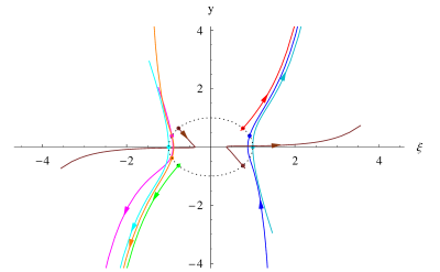
Figure 1: An example of section of the 4D phase space obtained with numerical calculations. We can see a series of trajectories corresponding to different choices of the initial conditions. Every initial condition in the graphic is chosen on the dashed “ellipse” centered in the origin and is emphasized by a colored dot. A “saddle point-like” structure of the set of the trajectories clearly emerges.

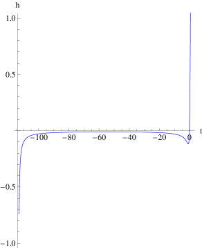
Figure 2: Typical behavior of the Hubble parameter for the model I trajectories. The presence of two stationary points (namely a maximum followed by a minimum) indicates the double crossing of the phantom divide line. Both the initial and final singularities are characterized by a Big Rip behavior, the first is a contraction and the second is an expansion.

Now, we describe some results of numerical calculations to have an idea about the structure of the set of possible cosmological evolutions coexisting in the model under consideration. We have carried out two kinds of simulations. First, we have considered neighborhood of the plane $y,\xi$ with the initial conditions on the field $\phi$ such that $\phi(0)=0,\dot{\phi}(0)=0$ (see Figure 1). The initial conditions for the phantom field were chosen in such a way that the sum of absolute values of the kinetic and potential energies were fixed. Then, running the time back and forward we have seen that the absolute majority of the cosmological evolutions began at the singularity of the “anti-Big Rip” type (Figure 2). Namely, the initial cosmological singularity were characterized by an infinite value of the cosmological radius and an infinite negative value of its time derivative (and also of the Hubble variable). Then the universe squeezes, being dominated by the phantom scalar field $\xi$. At some moment the universe passes the phantom divide line and the universe continues squeezing but with $\dot{h}<0$. Then it achieves the minimal value of the cosmological radius and an expansion begins. At some moment the universe undergoes the second phantom divide line crossing and its expansion becomes super-accelerated culminating in an encounter with a Big Rip singularity. Apparently this scenario is very different from the standard cosmological scenario and with its phantom version Bang-to-Rip, which has played a role of an input in the construction of our potentials. The second procedure, which we have used is the consideration of trajectories close to our initial trajectory of the Bang-to-Rip type. The numerical analysis shows that this trajectory is unstable and the neighboring trajectories again have anti-Big Rip - double crossing of the phantom line - Big Rip behavior described above. However, it is necessary to emphasize that a small subset of the trajectories of the Bang-to-Rip type exist, being not in the vicinity of our initial trajectory.

3.2 Model II

In this subsection we shall study the cosmological model with the potential (58). Now the system of equations (67) looks like

$$\left\{\begin{array}[]{ll}\dot{\phi}=&x,\\ \dot{\xi}=&y,\\ \dot{x}=&-3{\rm sign}(h)x\sqrt{\frac{x^{2}}{2}-\frac{y^{2}}{2}+\frac{2}{9t_{R}^{2}}\cosh^{6}(3\phi/4)\exp\{3\sqrt{2}\xi\}}\\ &-\frac{1}{t_{R}^{2}}\cosh^{5}(3\phi/4)\sinh(3\phi/4)e^{3\sqrt{2}\xi},\\ \dot{y}=&-3{\rm sign}(h)y\sqrt{\frac{x^{2}}{2}-\frac{y^{2}}{2}+\frac{2}{9t_{R}^{2}}\cosh^{6}(3\phi/4)\exp\{3\sqrt{2}\xi\}}\\ &+\frac{2\sqrt{2}}{3t_{R}^{2}}\cosh^{6}(3\phi/4)e^{3\sqrt{2}\xi}.\par\end{array}\right.$$ (77)

Notice that the potential (58) has an additional reflection symmetry

$$V_{2}(\xi,\phi)=V_{2}(\xi,-\phi).$$ (78)

This provides the symmetry with respect to the origin in the plane $(\phi,x)$. The system (77) has no stationary points. However, there is an interesting point

$$\phi=0,\ x=0,$$ (79)

which freezes the dynamics of $\phi$ and hence, permits to consider independently the dynamics of $\xi$ and $y$, described by the subsystem

$$\left\{\begin{array}[]{ll}\dot{\xi}=&y,\\ \dot{y}=&-3{\rm sign}(h)y\sqrt{-\frac{y^{2}}{2}+\frac{2}{9t_{R}^{2}}e^{3\sqrt{2}\xi}}+\frac{2\sqrt{2}}{3t_{R}^{2}}e^{3\sqrt{2}\xi}.\end{array}\right.$$ (80)

Apparently, the evolution of the universe is driven now by the phantom field and is subject to superacceleration.

In this case the qualitative analysis of the differential equations for $\xi$ and $y$, confirmed by the numerical simulations gives a predictable result: being determined by the only phantom scalar field the cosmological evolution is characterized by the growing positive value of $h$. Namely, the universe begins its evolution from the anti-Big Rip singularity ($h=-\infty$) then $h$ is growing passing at some moment of time the value $h=0$ (the point of minimal contraction of the cosmological radius $a(t)$) and then expands ending its evolution in the Big Rip cosmological singularity ($h=+\infty$).

Another numerical simulation can be done by fixing initial conditions for the phantom field as $\xi(0)=0,y(0)=0$ (see Figure 3). Choosing various values of the initial conditions for the scalar field $\phi(0),x(0)$ around the point of freezing $\phi=0,x=0$ we found two types of cosmological trajectories:
1. The trajectories starting from the anti-Big Rip singularity and ending in the Big Rip after the double crossing of the phantom divide line. These trajectories are similar to those discussed in the preceding subsection for the model I.
2. The evolutions of the type Bang-to-Rip.

Then we have carried out the numerical simulations of cosmological evolutions, choosing the initial conditions around the point of the phantomization point with the coordinates

$$\phi(0)=0,$$

$$x(0)=\frac{\sqrt{2}}{3},$$

$$\xi(0)=\frac{4}{3}{\rm arctanh}\frac{1}{\sqrt{2}},$$

$$y(0)=\frac{\sqrt{2}}{3}.$$ (81)

This analysis shows that in contrast to the model I, here the standard phantomization trajectory is stable and the trajectories of the type Bang-to-Rip are not exceptional, though less probable then those of the type anti-Big Rip to Big Rip.

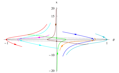
Figure 3: An example of section of the 4D phase space for the model II obtained with numerical calculations. We can see a family of different trajectories corresponding to different choices of the initial conditions. Every initial condition in the graphic is chosen on the dashed “ellipse”. The origin represents the point of freezing.

4 Conclusion

We have considered the problem of reconstruction of the potential in a theory with two scalar fields (one standard and one phantom) starting with a given cosmological evolution. It is known ( see e.g. [15, 16, 17]) that in the case of the only scalar field this potential is determined uniquely as well as the initial conditions for the scalar field, reproducing the given cosmological evolution. Changing the initial conditions, one can find a variety of cosmological evolutions, sometimes qualitatively different from the “input” one (see e.g. [17]). In the case of two fields the procedure of reconstruction becomes much more involved. As we have shown here, there is a huge variety of different potentials reproducing the given cosmological evolution (a very simple one in the case, which we have explicitly studied here). Every potential entails different cosmological evolutions, depending on the initial conditions.

It is interesting that the existence of different dynamics of scalar fields corresponding to the same evolution of the Hubble parameter $h(t)$ can imply some observable consequences connected with the possible interactions of the scalar fields with other fields. Indeed, in this case, the time dependence of the scalar fields considered above can directly affect physically observable quantities. We are going to consider this topic elsewhere [25].

References

References

- [1] Riess A et al. 1998 Astron. J. 116 1009; Perlmutter S J et al. 1999 Astroph. J. 517, 565.
- [2] Sahni V and Starobinsky A A 2000 Int. J. Mod. Phys. D 9 373; Padmananbhan T 2003 Phys. Rep. 380 235; Peebles P J E and Ratra B 2003 Rev. Mod. Phys. 75 559; Sahni V 2002 Class. Quantum Grav. 19 3435; Copeland E J, Sami M and Tsujikawa S 2006 Int. J. Mod. Phys. D 15 1753; Sahni V and Starobinsky A A 2006 Int. J. Mod. Phys. D 15 2105.
- [3] Caldwell R R, Dave R and Steinhardt P J 1998 Phys. Rev. Lett. 80 1582; Frieman J A, Waga I 1998 Phys. Rev. D 57 4642.
- [4] Armendariz-Picon C, Damour T and Mukhanov V 1999 Phys. Lett. B 458 209; Armendariz-Picon C, Mukhanov V and Steinhardt P J 2000 Phys. Rev. Lett. 85 4438; Armendariz-Picon C, Mukhanov V, Steinhardt P J 2001 Phys. Rev. D 63 103510; Chiba T, Okabe T, Yamaguchi M 2000 Phys. Rev. D 62 023511; Kamenshchik A, Moschella U and Pasquier V 2001 Phys. Lett. B 511 265; Bilic N, Tupper G B, and Violeer R 2002 Phys. Lett. B 535 17; Fabris J C, Gonsalves V B and de Souza P E 2002 Gen. Rel. Grav. 34 53; Bento M C, Bertolami O and Sen A A 2002 Phys. Rev. D 66 043507; Gorini V, Kamenshchik A and Moschella U 2003 Phys. Rev. D 67 063509; Sen A 2002 JHEP 0204 048; Gibbons G W 2002 Phys. Lett. B 537 1; Fairbairn M and Tytgat M H G 2002 Phys. Lett. B 546 1; Mukohyama S 2002 Phys. Rev. D 66 024009; Padmanabhan T and Choudhury T R 2002 Phys. Rev. D 66 081301(R); Sami M, Chingangbam P and Qureshi T 2002 Phys. Rev. D 66 043530; Felder G N, Kofman L and Starobinsky A A 2002 JHEP 0209 026; Frolov A, Kofman L and Starobinsky A 2002 Phys. Lett. B 545 8; Padmanabhan T 2002 Phys. Rev. D 66 021301(R); Feinstein A 2002 Phys. Rev. D 66 063511; Abramo L W and Finelli F 2003 Phys. Lett. B 575 165; Bagla J S, Jassal H K and Padmanabhan T 2003 Phys. Rev. D 67 063504; Gibbons G 2003 Class. Quant. Grav. 20 S321; Causse M B A rolling tachyon field for both dark energy and dark halos of galaxies Preprint astro-ph/0312206; Paul B C and Sami M 2004 Phys. Rev. D 70 027301; Sen A 2005 Phys. Scripta T 117 70; Garousi M R, Sami M and Tsujikawa S 2004 Phys. Rev. D 70 043536; Calcagni G 2004 Phys. Rev. D 69 103508; Aguirregabiria J M and Lazkoz R 2004 Mod. Phys. Lett. A 19 927; Aguirregabiria J M and Lazkoz R 2004 Phys. Rev. D 69 123502; Herrera R, Pavon D and Zimdahl W 2004 Gen. Rel. Grav. 36 2161; Barnaby N 2004 JHEP 0407 025; Allemandi G, Borowiec A and Francaviglia M 2004 Phys. Rev. D 70 043524; Zimdahl W Interacting Dark Energy and Cosmological Equations of State Preprint gr-qc/0505056; Allemandi G, Borowiec A, Francaviglia M and Odintsov S D 2005 Phys. Rev. D 72 063505.
- [5] Cooper F and Venturi G 1981 Phys. Rev. D 24 3338; Ratra B and Peebles P J E 1988 Phys. Rev. D 37 3406; Peebles P J E and Ratra B 1988 Astrophys. J. Lett. 325 L17; Wetterich C 1988 Nucl. Phys. B 302 668.
- [6] Caldwell R R 2002 Phys. Lett. B 545 23; Gonzalez-Diaz P F Phys. Lett. B 586 1; Singh P, Sami M and Dadhich N Phys. Rev. D 68 023522; Nojiri S and Odintsov S D Phys. Lett. B 562 147; Capozziello S, Nojiri S and Odintsov S D Phys. Lett. B 632 597; Johri V B 2004 Phys. Rev. D 70 041303(R); Onemli V K and Woodard R P 2000 Class. Quant. Grav. 19 4607; Hannestad S and Mortsell E 2002 Phys. Rev. D 66 063508; Carroll S M, Hoffman M and Trodden M Phys. Rev. D 68 023509; Frampton P H Stability Issues for Dark Energy Preprint hep-th/0302007; Elizalde E, Nojiri S and Odintsov S D Phys. Rev. D 70 043539; Gonzalez-Diaz P F and Siguenza C L 2004 Nucl. Phys. B 697 363; Gibbons G W Phantom Matter and the Cosmological Constant Preprint hep-th/0302199; McInnes B What If ? Preprint astro-ph/0210321; Chimento L P and Lazkoz R 2003 Phys. Rev. Lett. 91 211301; Dabrowski M P, Stachowiak T and Szydlowski M 2003 Phys. Rev. D 68 103519; Singh P, Sami M and Dadhich N 2003 Phys. Rev. D 68 023522; Gonzalez-Diaz P F 2004 Phys. Rev. D 69 063522; Onemli V K and Woodard R P 2004 Phys. Rev. D 70 107301; Sami M and Toporensky A 2004 Mod. Phys. Lett. A 19 1509; Stefancic H 2004 Eur. Phys. J. C 36 523; Stefancic H 2004 Phys. Lett. B 586 5; Brunier T, Onemli V K and Woodard R P 2005 Class. Quantum Grav. 22 59; Santos J and Alcaniz J S 2005 Phys. Lett. B 619 11; Carvalho F C and Saa A 2004 Phys. Rev. D 70 087302; Melchiorri A, Mersini L, Odman C J and Trodden M 2003 Phys. Rev. D 68 043509; Cline J M, Jeon S and Moore J D 2004 Phys. Rev. D 70 043543; Guo Z K, Piao Y S, Zhang X M and Zhang Y Z 2005 Phys. Lett. B 608 177; Feng B, Wang X L and Zhang X M 2005 Phys. Lett. B 607 35; Aref’eva I Y, Koshelev A S and Vernov S Y Exactly Solvable SFT Inspired Phantom Model to be published in Theor. Math. Phys. Preprint astro-ph/0412619; Zhang X F, Li H, Piao Y S and Zhang X M Two-field Models of Dark Energy with Equation of State Across -1 Preprint astro-ph/0501652; Calcagni G 2005 Phys. Rev. D 71 023511; Li M, Feng B and Zhang X 2005 JCAP 0512 002; Babichev E, Dokuchaev V and Eroshenko Yu 2005 Class. Quant. Grav. 22 143; Anisimov A, Babichev E and Vikman A 2005 JCAP 0506 006; Nojiri S, Odintsov S D and Tsujikawa S 2005 Phys. Rev. D 71 063004; Gumjudpai B, Naskar T, Sami M and Tsujikawa S 2005 JCAP 0506 007; Sami M, Toporensky A, Tretjakov P V and Tsujikawa S 2005 Phys. Lett. B 619 193; Nojiri S and Odintsov S D 2006 Gen. Relativ. Grav. 38 1285; Brevik I 2006 Gen. Relativ. Grav. 38 1317.
- [7] Alam U, Sahni V, Saini T D and Starobinsky A A 2004 Mon. Not. Roy. Astron. Soc. 354 275; Padmanabhan T and Choudhury T R 2003 Mon. Not. Roy. Astron. Soc. 344 823; Choudhury T R and Padmanabhan T 2005 Astron.Astrophys. 429 807; Wang Y and Mukherjee P 2004 Astrophys. J. 606 654; Huterer D and Cooray A 2005 Phys. Rev. D 71 023506; Daly R A and Djorgovski S G 2003 Astrophys. J. 597 9; Alcaniz J S 2004 Phys. Rev. D 69 083521; Lima J A S, Cunha J V and Alcaniz J S 2003 Phys. Rev. D 68 023510; Alam U, Sahni V and Starobinsky A A 2004 JCAP 0406 008; Wang Y and Freese K 2006 Phys. Lett. B 632449; Upadhye A, Ishak M and Steinhardt P J 2005 Phys. Rev. D 72 063501; Dicus D A and Repko W W 2004 Phys. Rev. D 70 083527; Espana-Bonet C and Ruiz-Lapuente P Dark Energy as an Inverse Problem Preprint hep-ph/0503210; Wei Y H The power-law expansion universe and dark energy evolution Preprint astro-ph/0405368; Jassal H K, Bagla J S, and Padmanabhan T 2005 Mon. Not. Roy. Astron. Soc. Letters 356 L11; Nesseris S and Perivolaropoulos L 2004 Phys. Rev. D 70 043531; Lazkoz R, Nesseris S and Perivolaropoulos L 2005 JCAP 0511 010; Jassal H K, Bagla J S and Padmanabhan T 2005 Phys. Rev. D 72 103503; Feng B, Li M, Piao Y S and Zhang X 2006 Phys. Lett. B 634 101-105; Xia J Q, Feng B and Zhang X M 2005 Mod. Phys. Lett. A 20 2409.
- [8] Cabre A, Gaztanaga E, Manera M, Fosalba P and Castander F 2006 Mon. Not. Roy. Astron. Soc. Lett. 372 L23-L27.
- [9] Barger V, Gao Y and Marfatia D 2007 Phys. Lett. B 648 127; Gong A and Wang A 2007 Phys. Rev. D 75 0435520; Alam U, Sahni V and Starobinsky A A 2007 JCAP 0702 011; Nesseris S and Perivolaropoulos L 2007 JCAP 0702 025; Zhao G B, Xia J Q, Li H et al. Probing for dynamics of dark energy and curvature of universe with latest cosmological observations Preprint astro-ph/0612728; Serra P, Heavens A and Melchiorri A 2007 MNRAS 379 1,169; Davis T M, Mortsell E, Sollerman J et al. Scrutinizing Exotic Cosmological Models Using ESSENCE Supernova Data Combined with Other Cosmological Probes Preprint astro-ph/0701510; Wright E L Constraints on Dark Energy from Supernovae, Gamma Ray Bursts, Acoustic Oscillations, Nucleosynthesis and Large Scale Structure and the Hubble constant Preprint astro-ph/0701584; Wang Y and Mukherjee P Observational Constraints on Dark Energy and Cosmic Curvature Preprint astro-ph/0703780.
- [10] Boisseau B, Esposito-Farese G, Polarski D and Starobinsky A A 2000 Phys. Rev. Lett. 85 2236; Esposito-Farese G and Polarski D 2001 Phys. Rev. D 63 063504; Vikman A 2005 Phys. Rev. D 71 023515; Perivolaropoulos L 2005 Phys. Rev. D 71 063503; McInnes B 2005 Nucl. Phys. B 718 55; Aref’eva I Ya, Koshelev A S and Vernov S Yu 2005 Phys. Rev. D 72 064017; Perivolaroupoulos L 2005 JCAP 0510 001; Caldwell R R and Doran M 2005 Phys. Rev. D 72 043527; Sahni V and Shtanov Yu 2003 JCAP 0311 014; Sahni V and Wang L 2000 Phys. Rev. D 62 103517; Wei H, Cai R G and Zeng D F 2005 Class. Quant. Grav. 22 3189; Wei H, Cai R G 2005 Phys. Rev. D 72 123507; Wei H, Cai R G 2006 Phys. Lett. B 634 9; Cai R G and Wang A 2005 JCAP 0503 002; Gannouji R, Polarski D, Ranquet A and Starobinsky A A 2006 JCAP 0609 016.
- [11] Andrianov A A, Cannata F and Kamenshchik A Y 2005 Phys. Rev. D 72 043531.
- [12] Cannata F and Kamenshchik A Yu Networks of cosmological histories, crossing of the phantom divide line and potentials with cusps (to appear in Int. J. Mod. Phys. D) Preprint gr-qc/0603129.
- [13] Andrianov A A, Cannata F and Kamenshchik A Yu 2006 Int. J. Mod. Phys. D 15 1299; Andrianov A A, Cannata F and Kamenshchik A Yu 2006 J. Phys. A 39 9975.
- [14] Feng B, Wang X and Zhang X 2005 Phys. Lett. B 607 35; Guo Z K, Piao Y S, Zhang X and Zhang Y Z 2005 Phys. Lett. B 608 177; Hu W 2005 Phys. Rev. D 71 047301; Perivolaropoulos L 2005 Phys. Rev. D 71 063503; Caldwell R R and Doran M 2005 Phys. Rev. D 72 043527.
- [15] Starobinsky A A 1998 JETP Lett. 68 757.
- [16] Burd A B and Barrow J D 1988 Nucl. Phys. B 308 929; Barrow J D 1990 Phys. Lett. B 235 40.
- [17] Gorini V, Kamenshchik A, Moschella U and Pasquier V 2004 Phys. Rev. D 69 123512.
- [18] Zhuravlev V M, Chervon S V and Shchigolev V K 1998 JETP 87 223; Chervon S V and Zhuravlev V M The cosmological model with an analytic exit from inflation Preprint gr-qc/9907051; Yurov A V Phantom scalar fields result in inflation rather than Big Rip Preprint astro-ph/0305019; Yurov A V and Vereshchagin S D 2004 Theor. Math. Phys. 139 787.
- [19] Guo Z K, Ohta N and Zhang Y Z 2007 Mod. Phys. Lett. A 22 883; Guo Z K, Ohta N and Zhang Y Z 2005 Phys. Rev. D 72 023504.
- [20] Zhuk A 1996 Class. Quant. Grav. 13 2163.
- [21] Szydlowski M and Czaja W 2004 Phys. Rev. D 69 083507; Szydlowski M and Czaja W 2004 Phys. Rev. D 69 083518; Szydlowski M 2005 Int. J. Mod. Phys. A 20 2443; Szydlowski M, Hrycyna O and Krawiec A 2007 JCAP 0706 010.
- [22] Vernov S Yu Construction of Exact Solutions in Two-Fields Models and the Crossing of the Cosmological Constant Barrier Preprint astro-ph/0612487.
- [23] Regoli D 2007 Mg. Thesis University of Bologna (in Italian).
- [24] Belinsky V A, Khalatnikov I M, Grishchuk L P and Zeldovich Ya B 1985 Sov. Phys. JETP 62 195; Belinsky V A, Khalatnikov I M, Grishchuk L P and Zeldovich Ya B 1985 Phys. Lett. B 155 232.
- [25] Andrianov A A, Cannata F, Kamenshchik A Yu and Regoli D, work in progress.