Transverse-momentum-dependent parton distribution function in soft-collinear effective theory

Abstract

Transverse-momentum-dependent parton distribution functions are analyzed in semi-inclusive deep inelastic scattering at low transverse momentum using soft-collinear effective theory. The transverse-momentum-dependent parton distribution functions are defined on the lightcone without distorting the lightcone path nor adding additional soft Wilson lines. In this approach, the comparison between the integrated and unintegrated parton distribution functions becomes transparent. The procedure of computing radiative corrections in dimensional regularization is explained in detail, and the divergence, which is a product of infrared and ultraviolet divergence, is cancelled. The renormalization group equation for the transverse-momentum-dependent parton distribution functions is derived. It depends only on the relevant physical quantities and exhibits a nontrivial scaling behavior because the longitudinal momentum fraction and the transverse momentum are coupled in the renormalization group equation.

I Introduction

High-energy scattering cross sections are usually expressed in a factorized form, in which the hard scattering kernel and the parton distribution functions (and the fragmentation functions if semi-inclusive or exclusive scattering is considered) are convoluted. The factorization property reflects the idea of separating long-distance and short-distance physics in high-energy scattering. The hard scattering occurs independent of the details about how energetic partons are produced or how final-state particles hadronize, and vice versa. Theoretically the factorization implies that each factorized part can be treated separately. The hard scattering kernel can be computed using perturbative QCD. Parton distribution functions describe the nonperturbative nature of partons to have a certain fraction of longitudinal momentum inside an incoming hadron, hence not computable in perturbation theory. But their evolution with respect to the factorization scale $\mu$ can be computed. The factorization property is the basis to study many high energy processes.

In inclusive high-energy processes, only integrated parton distribution functions (i.e., parton distribution functions integrated over the transverse momentum) are needed to be convoluted with the hard scattering kernel. The integrated parton distribution functions can be well defined in a gauge-invariant way as the matrix elements of the relevant operators and their evolutions are described by the renormalization group equation. If we consider semi-inclusive or exclusive processes, that is, if one or more final-state particles are tagged, more detailed information on the scattering such as the transverse momentum dependence or spin correlations can be probed, but it is more complicated than inclusive processes. In this case, the scattering cross section is convoluted with one more nonperturbative fragmentation function, which contains the information on the hadronization effect. However, since the transverse-momentum-dependent (TMD) parton distribution function (PDF) was proposed Collins:1981uk ; Collins:1981uw , its definition and, accordingly, its radiative corrections are known to cause severe problems Collins:2003fm . These problems are related to the failure of showing the cancellation of divergences between real gluon emission and virtual gluon exchange in certain calculational schemes once the TMD PDF is defined. The issues can be categorized into the definition of the TMD PDF, the choice of gauge (axial or covariant), and the regularization schemes though they are intertwined with each other. In this paper, the aspect of the transverse momentum dependence in semi-inclusive deep inelastic scattering (SIDIS) is considered and the spin correlation is not treated. TMD PDF has attracted a lot of attention since its effect can be detected in experiments.

The problem can be described as follows Collins:2003fm : The TMD (or unintegrated) quark distribution function $f(x,{\bf k}_{\perp})$ at one loop is written as

$$f^{(1)}(x,{\bf k}_{\perp})=P_{1R}(x,{\bf k}_{\perp})-\delta(1-x)\delta({\bf k}_{\perp})\int dx^{\prime}d^{2}{\bf k}_{\perp}^{\prime}P_{1R}(x^{\prime},{\bf k}_{\perp}^{\prime}),$$ (1)

where $x$ is the lightcone momentum fraction and ${\bf k}_{\perp}$ is the transverse momentum. The quantity $P_{1R}$ is the real gluon emission amplitude at order $\alpha_{s}$, schematically given by

$$P_{1R}(x,{\bf k}_{\perp})\sim\alpha_{s}\Bigl{[}\frac{1}{1-x}\frac{1}{{\bf k}_{\perp}^{2}+\Delta^{2}}+\mathrm{regular\ as}\ x\rightarrow 1\Bigr{]},$$ (2)

where $\Delta^{2}$ involves the infrared regulator such as small quark and gluon masses, and the second term in Eq. (1) corresponds to the virtual gluon emission. It is argued that for any ${\bf k}_{\perp}$, there is an endpoint singularity as $x\rightarrow 1$, and there is no cancellation between the real gluon emission and the virtual gluon contribution. If the calculation is performed in light-cone gauge, the divergence arises from the $1/k_{+}$ singularity in the gluon propagator.

There have been several approaches to solving this problem. First, Collins and Soper Collins:1981uk proposed a non-gauge-invariant definition for the TMD PDF, and chose the axial gauge $n\cdot A=0$, but with a non-lightlike gauge fixing vector $n^{\mu}$. As a result, a rapidity parameter $\zeta=(p\cdot n)^{2}/n^{2}$ ($n^{2}\neq 0$) was introduced and an additional evolution equation of the PDF on this parameter was developed requiring that physical quantities like scattering cross sections are independent of this scale. But the computation off the lightcone is complicated, and the factorization property and the relation to the integrated PDF are not clear in this approach Ji:2004wu . Collins and Hautmann Collins:1999dz suggested to put Wilson lines on the lightcone and redefine the TMD PDF by adding additional soft Wilson lines to remove the divergence. They used method of regions to determine which kinematic regions yield divergences, and found subtraction terms to remove the divergence. From the explicit one-loop computation, they found additional soft Wilson lines slightly off the lightcone to be inserted in the gauge invariant definition of the TMD PDF. Cherednikov and Stefanis Cherednikov:2007tw redefined the TMD PDF by inserting a transverse gauge link which provides an additional soft counterterm. This additional term has the effect of cancelling the unwanted divergence related to the cusped contour. All the approaches try to define TMD or unintegrated PDF in a gauge-invariant way, and put some additional Wilson lines off the lightcone (taking the limit to the lightcone, if possible) in order to remove the problematic singularity mentioned above with the extra Wilson lines.

Soft-collinear effective theory (SCET) Bauer:2000ew ; Bauer:2000yr ; Bauer:2001yt is the theoretical framework which is appropriate for describing energetic particles. SCET has been applied successfully in $B$ decays and in other high-energy processes Bauer:2002nz such as deep inelastic scattering Manohar:2003vb ; Chay:2005rz ; Becher:2006mr ; Chen:2006vd ; Idilbi:2007ff . It can be also applied to SIDIS to describe the TMD PDF. The factorization property of SIDIS cross sections can be proved in a transparent way since the decoupling of collinear and soft degrees of freedom can be made manifest in the formulation of SCET. The TMD PDF can be defined in a gauge-invariant way putting all the Wilson lines on the lightcone without introducing extra Wilson lines off the lightcone. The computational technique developed in SCET offers an improved regularization method to show that the problem of the divergence is solved. The divergence appearing in Eqs. (1) and (2) is the mixture of ultraviolet and infrared divergences, which should not be present for physical quantities. In order to show the cancellation of the divergence using dimensional regularization, care must be taken to extract $\delta(1-x)$ in Eq. (1). In this paper, the cancellation of the mixed divergence is explicitly presented. In Section II, kinematics relevant to SIDIS is briefly considered and the current operators in SCET for SIDIS are introduced. In Section III, the TMD PDF and TMD soft Wilson lines are defined in terms of the matrix elements of the relevant operators. And the factorization of the hadronic tensor as a convolution of the fragmentation function and the TMD PDF is established. The TMD PDF itself is a convolution of the matrix elements for the collinear operator and the soft Wilson line. And the relation between the TMD and integrated PDF is explained. In Section IV, the radiative corrections for the TMD collinear operator and the TMD soft Wilson lines are computed at one loop. In Sec. V, the renormalization group equations for the TMD collinear operator, the TMD soft Wilson line, hence for the TMD PDF are presented. In Section VI, a conclusion is given.

II Kinematics

In order to discuss TMD PDF, a reference frame should be selected first to define what transverse momentum is referred to. In SIDIS such as $e+p\rightarrow e+h+X$, where $h$ is an energetic tagged final-state hadron and $X$ denotes all the remaining final states, the reference frame is chosen such that the spatial components of the momentum transfer $q^{\mu}$ from the leptonic system and the proton momentum $P^{\mu}$ lie in the $z$ axis. In this frame, the momenta $q^{\mu}$ and $P^{\mu}$ can be written as

$$q^{\mu} = (\overline{n}\cdot q,{\bf q}_{\perp},n\cdot q)=(Q,{\bf 0}_{T},-Q),$$

$$P^{\mu} = P_{\bar{n}}^{\mu}=(\overline{n}\cdot P,{\bf P}_{\perp},n\cdot P)\sim(\Lambda^{2}/Q,{\bf 0}_{T},Q),$$ (3)

where $q^{2}=-Q^{2}$, and $\Lambda$ is a typical hadronic scale. The lightlike vectors $n^{\mu}$ and $\overline{n}^{\mu}$ satisfy $n^{2}=\overline{n}^{2}=0$, and $n\cdot\overline{n}=2$. We can set $n^{\mu}=(1,0,0,1)$ and $\overline{n}^{\mu}=(1,0,0,-1)$, and the proton moves in the $\overline{n}$ ($-z$) direction with this choice. Note that an individual parton inside a proton can have nonzero transverse momentum of order $\Lambda$ due to the fluctuation inside a proton, though the proton has no transverse momentum. We will consider the case in which the transverse momentum of the final-state particle is of order $\Lambda$. Of course, the outgoing hadron can have transverse momentum much larger than $\Lambda$. But in this case, we know from the momentum conservation that there should be other final-state particles with large transverse momenta such that the final transverse momenta add up to be of order $\Lambda$. Technically, as will be seen later, if the final hadron has a large transverse momentum, it is extracted as a label momentum. Then the large transverse momentum and the transverse momentum of order $\Lambda$ are treated separately. Due to momentum conservation in each subspace of the transverse momenta, the final result can be derived in a similar way as in the case in which the final-state hadron is in the $n$ direction with small transverse momentum of order $\Lambda$. For this reason, we consider the final-state hadron with $n$-collinear momentum $P_{n}$ and small transverse momentum from now on for simplicity, noting that the case with large transverse momentum can be treated in a straightforward way.

At the hadronic level, we can define the invariants in terms of $Q$, $P_{\bar{n}}$ and the outgoing hadron momentum $P_{n}$ as

$$x_{H}=\frac{Q^{2}}{2P_{\bar{n}}\cdot q}=\frac{Q}{n\cdot P_{\bar{n}}},\ \ z_{H}=\frac{P_{\bar{n}}\cdot P_{n}}{P_{\bar{n}}\cdot q}=\frac{\overline{n}\cdot P_{n}}{Q}.$$ (4)

Defining the momentum fractions $\xi$ and $\xi^{\prime}$ of the partons to hadrons as $n\cdot p_{\bar{n}}=\xi n\cdot P_{\bar{n}}$ and $\xi^{\prime}\overline{n}\cdot p_{n}=\overline{n}\cdot P_{n}$, the corresponding partonic invariants are given by

$$x=\frac{x_{H}}{\xi}=\frac{Q}{n\cdot p_{\bar{n}}},\ \ z=\frac{z_{H}}{\xi^{\prime}}=\frac{\overline{n}\cdot p_{n}}{Q},$$ (5)

where the momenta of the incoming and outgoing partons are in the $\overline{n}^{\mu}$, $n^{\mu}$ directions respectively such that

$$p_{\bar{n}}^{\mu} = (\overline{n}\cdot p_{\bar{n}},{\bf p}_{\bar{n}\perp},n\cdot p_{\bar{n}})\sim\Bigl{(}\displaystyle\frac{x\Lambda^{2}}{Q},\Lambda,\frac{Q}{x}\Bigr{)},$$

$$p_{n}^{\mu} = (\overline{n}\cdot p_{n},{\bf p}_{n\perp},n\cdot p_{n})\sim\Bigl{(}\displaystyle zQ,\Lambda,\frac{\Lambda^{2}}{zQ}\Bigr{)}.$$ (6)

The scale $Q$ sets the large scale in the system, and there is a hierarchy of scales in the momentum components such that

$$p_{\bar{n}}^{\mu}\sim Q(\lambda^{2},\lambda,1),\ \ p_{n}^{\mu}\sim Q(1,\lambda,\lambda^{2}),$$ (7)

where $\lambda\sim\Lambda/Q$, and SCET describes the dynamics of these particles. With this choice of the reference frame, the incoming partons and the outgoing parton can have transverse momenta of order $\Lambda$ with respect to the axis on which the incoming proton and the photon lie.

The electroproduction in SIDIS is mediated by the electromagnetic current operator of the form $\overline{\psi}\gamma^{\mu}\psi$. The corresponding electromagnetic current operator in SCET is given by

$$j_{\mu}(x) = C(Q,\mu)e^{i(\overline{n}\cdot p_{n}n\cdot x/2-n\cdot p_{\bar{n}}\overline{n}\cdot x/2)}\overline{\chi}_{n}Y_{n}^{\dagger}\gamma_{\perp\mu}Y_{\bar{n}}\chi_{\bar{n}}(x),$$

$$j^{\dagger}_{\mu}(x) = C(Q,\mu)e^{-i(\overline{n}\cdot p_{n}n\cdot x/2-n\cdot p_{\bar{n}}\overline{n}\cdot x/2)}\overline{\chi}_{\bar{n}}\tilde{Y}^{\dagger}_{\bar{n}}\gamma_{\perp\mu}Y_{n}\chi_{n}(x),$$ (8)

where $C(Q,\mu)$ is the Wilson coefficient obtained by matching the current operator in the full theory onto SCET Manohar:2003vb

$$C(Q,\mu)=1+\frac{\alpha_{s}C_{F}}{4\pi}\Bigl{(}-\ln^{2}\frac{Q^{2}}{\mu^{2}}+3\ln\frac{Q^{2}}{\mu^{2}}-8+\frac{\pi^{2}}{6}\Bigr{)}.$$ (9)

A collinear fermion field in the $n$ direction can be obtained from the full theory as

$$\xi_{n}(x)=\sum_{\tilde{p}}e^{-i\tilde{p}\cdot x}\frac{\hbox{$/$}\kern-5.50117pt\hbox{$n$}\hbox{$/$}\kern-5.0pt\hbox{$\overline{n}$}}{4}\psi(x),$$ (10)

where $\tilde{p}^{\mu}=\overline{n}\cdot pn^{\mu}/2$ is the large label momentum. The field $\chi_{n}$, which is defined as $\chi_{n}=W_{n}^{\dagger}\xi_{n}$, is introduced to simplify notation, and $W_{n}$ is the collinear Wilson line given by

$$W_{n}=\sum_{\mathrm{perm}}\exp\Bigl{[}-g\frac{1}{\overline{n}\cdot\mathcal{P}}n\cdot A_{n}\Bigr{]},$$ (11)

where $\overline{n}\cdot\mathcal{P}$ is the operator extracting the label momentum. For $\overline{n}$ collinear particles, the corresponding quantities are obtained by switching $n$ and $\overline{n}$.

The collinear fields can be redefined to decouple from the soft fields as Bauer:2001yt

$$\xi_{n}(x)\rightarrow Y_{n}\xi_{n},\ A_{n}^{\mu}\rightarrow Y_{n}A_{n}^{\mu}Y_{n}^{\dagger}$$

$$\xi_{\bar{n}}(x)\rightarrow Y_{\bar{n}}\xi_{\bar{n}},\ A_{\bar{n}}^{\mu}\rightarrow Y_{\bar{n}}A_{\bar{n}}^{\mu}Y_{\bar{n}}^{\dagger},$$ (12)

where $Y_{n}$ and $Y_{\bar{n}}$ are soft Wilson lines. The form and the analytic structure of the soft Wilson lines can be determined from the direction of the underlying collinear particles, and depend on whether the collinear particle is a particle or an antiparticle Chay:2004zn . And the basic building blocks for the soft Wilson lines are given as

$$Y_{n}(x)=P\exp\Bigl{[}ig\int_{-\infty}^{x}dsn\cdot A_{s}(ns)\Bigr{]},\ \tilde{Y}_{n}(x)=\overline{P}\exp\Bigl{[}-ig\int_{x}^{\infty}dsn\cdot A_{s}(ns)\Bigr{]},$$ (13)

and their hermitian conjugates, where $P$ and $\overline{P}$ denote path and anti-path ordering respectively. In Eq. (II), the soft Wilson lines are chosen appropriate for deep inelastic scattering, as explained in detail in Ref. Chay:2004zn . The prescription of the soft Wilson lines is shown in Fig. 1 (a), which is equal to Fig. 1 (b) since the overlapping Wilson lines are cancelled.

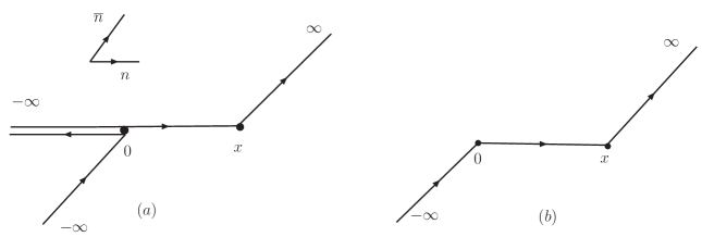
Figure 1: The prescription for the soft Wilson lines in deep inelastic scattering. (a) In the current $j_{\mu}^{\dagger}(x)$, $\xi_{n}$ from $-\infty$ to $x$, and $\xi_{\bar{n}}$ from $x$ to $\infty$. In $j_{\nu}(0)$, $\xi_{\bar{n}}$ from $-\infty$ to 0, and $\xi_{n}$ from 0 to $-\infty$. See Eq. (14). (b) The net soft Wilson line after the cancellation.

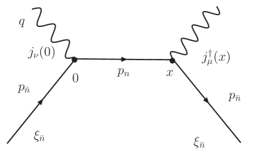
Figure 2: Feynman diagram for forward Compton scattering amplitude in deep inelastic scattering. The scattering cross section is proportional to the discontinuity of the intermediate states by the optical theorem.

There exist other equivalent prescriptions for the soft Wilson lines, but the procedure of calculating anomalous dimensions should also be prescribed. The above prescription is for the forward Compton scattering amplitude in deep inelastic scattering. (See Fig. 2.) This prescription is simple in the sense that the same Feynman rules can be used anywhere in Feynman diagrams, and it makes the calculation of the anomalous dimension straightforward. Note that the choice of the directions for the underlying collinear particles such as forward scattering amplitude applies only to the prescription for the soft Wilson lines, not to the actual processes. In other prescriptions, the same result can be reached, but by a different procedure. For example, if soft Wilson lines are prescribed with a matrix element squared for a scattering cross section instead of the time-ordered product for the forward scattering amplitude, different Feynman rules should be applied across the cut to produce the desired result Collins:1981uk , or the cusp angle in computing the anomalous dimension should be inverted in the complex conjugate part at the final step Korchemsky:1992xv .

III TMD parton distribution functions and soft Wilson lines

Consider the hadronic tensor, which is defined as

$$W_{\mu\nu}=\sum_{X}\int d^{4}xe^{iq\cdot x}\langle P|j_{\mu}^{\dagger}(x)|Xh\rangle\langle Xh|j_{\nu}(0)|P\rangle,$$ (14)

where the sum is over all the final states $X$ except the tagged hadron $h$. The SIDIS cross section is proportional to the hadronic tensor $W_{\mu\nu}$. It can be written in terms of the SCET current operators. The exponential factors extracting the label momenta all cancel due to momentum conservation requiring $x=z=1$ (or $\xi=x_{H}$, $\xi^{\prime}=z_{H}$), and it becomes

$$W_{\mu\nu} = C^{2}(Q)\int d^{4}x\sum_{X}\langle P_{\bar{n}}|\overline{\chi}_{\bar{n}}\tilde{Y}^{\dagger}_{\bar{n}}\gamma_{\perp\mu}Y_{n}\chi_{n}(x)|Xh\rangle\langle Xh|\overline{\chi}_{n}Y_{n}^{\dagger}\gamma_{\perp\nu}Y_{\bar{n}}\chi_{\bar{n}}(0)|P_{\bar{n}}\rangle$$ (15)

$$= C^{2}(Q)\int d^{4}x\sum_{X}\langle P_{\bar{n}}|\Bigl{(}\overline{\chi}_{\bar{n}}\gamma_{\perp\mu}\frac{\hbox{$/$}\kern-5.50117pt\hbox{$n$}}{2}\Bigr{)}_{i}^{a}\Bigl{(}\tilde{Y}^{\dagger}_{\bar{n}}Y_{n}\Bigr{)}^{ab}\Bigl{(}\frac{\hbox{$/$}\kern-5.0pt\hbox{$\overline{n}$}}{2}\chi_{n}\Bigr{)}_{i}^{b}(x)|Xh\rangle\langle Xh|\Bigl{(}\overline{\chi}_{n}\Bigr{)}_{k}^{c}$$

$$\times\Bigl{(}Y_{n}^{\dagger}Y_{\bar{n}}\Bigr{)}^{cd}\Bigl{(}\gamma_{\perp\nu}\chi_{\bar{n}}\Bigr{)}_{k}^{d}(0)|P_{\bar{n}}\rangle$$

where the color indices ($a$, $b$, $c$, $d$) and the Dirac indices ($i$, $j$, $k$) are explicitly shown in the last expression. The state $|P_{\bar{n}}\rangle$ denotes the proton state in SCET, which consists of $\overline{n}$-collinear partons.

Since there are no $\overline{n}$-collinear particles in the final state, the fragmentation function $D(z_{H},n\cdot r,r_{\perp})$ is defined as the average of the following matrix element over color and Dirac indices such that

$$\frac{1}{2N}\mathrm{Tr}\sum_{X}\langle 0|\Bigl{(}\frac{\hbox{$/$}\kern-5.0pt\hbox{$\overline{n}$}}{2}\chi_{n}(x)\Bigr{)}_{i}^{b}|Xh\rangle\langle Xh|\Bigl{(}\overline{\chi}_{n}(0)\Bigr{)}^{c}_{k}|0\rangle=\delta^{bc}\delta_{ik}\int\frac{d^{4}r}{(2\pi)^{4}}e^{-ir\cdot x}D(z_{H},n\cdot r,r_{\perp}),$$ (16)

where $D(z_{H},n\cdot r,r_{\perp})$ depends only on $n\cdot r$ and $r_{\perp}$ and the label momentum is given by $\overline{n}\cdot p_{n}=\overline{n}\cdot P_{n}/z_{H}$. The definition of the fragmentation function also holds when the final-state hadron $h$ has large transverse momentum after summing over all the final-state particles, though the partonic variables $x$ and $z$ can have values less than 1, and appropriate adjustments should be made accordingly. Note that, as in inclusive deep inelastic scattering, when the contribution of the final-state particles is all summed over, there is no dependence on the transverse momentum and it becomes the jet function $J_{P}(n\cdot r)$ Chay:2005rz , which depends only on $n\cdot r$. Therefore the transverse-momentum dependence in the fragmentation function, and subsequently in the PDF appears only when we specify at least one final-state particle with nonzero transverse momentum. From now on, the subscript in $z_{H}$ (and $x_{H}$) is dropped for simplicity with the understanding that the momentum fractions refer to the hadronic variables.

Using the fragmentation function, the hadronic tensor $W_{\mu\nu}=-g^{\perp}_{\mu\nu}W$ can be written, by integrating over $\overline{n}\cdot r$, as

$$W = \int d\omega C^{2}(\omega)\int\frac{d\overline{n}\cdot xd^{2}x_{\perp}}{2(2\pi)^{3}}\int dn\cdot rd^{2}r_{\perp}e^{-i(n\cdot r\overline{n}\cdot x/2+r_{\perp}\cdot x_{\perp})}D(z,n\cdot r,r_{\perp})$$ (17)

$$\times \langle P_{\bar{n}}|\overline{\chi}_{\bar{n}}(\overline{n}\cdot x,x_{\perp})\delta(\omega-\mathcal{P}_{+})\frac{\hbox{$/$}\kern-5.50117pt\hbox{$n$}}{2}\chi_{\bar{n}}(0)|P_{\bar{n}}\rangle\frac{1}{N}\langle 0|\mathrm{tr}\,\tilde{Y}^{\dagger}_{\bar{n}}Y_{n}(\overline{n}\cdot x,x_{\perp})Y_{n}^{\dagger}Y_{\bar{n}}(0)|0\rangle,$$

where the soft Wilson lines are extracted from the $\overline{n}$ states, since they are decoupled from the collinear part, and the color projection is taken. In Eq. (17), the delta function $\delta(\omega-\mathcal{P}_{+})$ is inserted explicitly with $\mathcal{P}_{+}=n\cdot\mathcal{P}+n\cdot\mathcal{P}^{\dagger}$ since the Wilson coefficient is actually an operator $C(n\cdot\mathcal{P},n\cdot\mathcal{P}^{\dagger})$. By expanding the operators with respect to $x_{\perp}$ and $\overline{n}\cdot x$, we obtain

$$\overline{\chi}_{\bar{n}}(0,x_{\perp})\frac{\hbox{$/$}\kern-5.50117pt\hbox{$n$}}{2}\delta(\omega-\mathcal{P}_{+})\chi_{\bar{n}}(0) = \int d^{2}k_{\perp}e^{-ik_{\perp}\cdot x_{\perp}}\overline{\chi}_{\bar{n}}\frac{\hbox{$/$}\kern-5.50117pt\hbox{$n$}}{2}\delta(\omega-\mathcal{P}_{+})\delta^{(2)}(k_{\perp}+i\partial_{\perp})\chi_{\bar{n}}(0),$$

$$\frac{1}{N}\mathrm{tr}\,\tilde{Y}^{\dagger}_{\bar{n}}Y_{n}(\overline{n}\cdot x,x_{\perp})Y_{n}^{\dagger}Y_{\bar{n}}(0) = \int d\eta d^{2}s_{\perp}e^{-i(\eta\overline{n}\cdot x/2+s_{\perp}\cdot x_{\perp})}$$ (18)

$$\times \frac{1}{N}\mathrm{tr}\,\tilde{Y}^{\dagger}_{\bar{n}}Y_{n}\delta(\eta+n\cdot i\partial)\delta^{(2)}(s_{\perp}+i\partial_{\perp})Y_{n}^{\dagger}Y_{\bar{n}}(0).$$

Note that the dependence of $\overline{\chi}_{n}$ on $\overline{n}\cdot x$ is dropped since the label momentum is already extracted, and the remaining momentum can be neglected. Then $W$ is written as

$$W = \int d\omega C^{2}(\omega)\int\frac{d\overline{n}\cdot xd^{2}x_{\perp}}{2(2\pi)^{3}}\int dn\cdot rd^{2}r_{\perp}\int d^{2}k_{\perp}\int d\eta d^{2}s_{\perp}$$ (19)

$$\times e^{-i(n\cdot r\overline{n}\cdot x/2+r_{\perp}\cdot x_{\perp})}e^{-ik_{\perp}\cdot x_{\perp}}e^{-i(\eta\overline{n}\cdot x/2+s_{\perp}\cdot x_{\perp})}D(z,n\cdot r,r_{\perp})\langle P_{\bar{n}}|\mathcal{O}_{c}(\omega,k_{\perp})|P_{\bar{n}}\rangle K(\eta,s_{\perp})$$

$$= \int d\omega C^{2}(\omega)\int dn\cdot rd^{2}r_{\perp}\int d^{2}k_{\perp}\int d\eta d^{2}s_{\perp}\delta(\eta+n\cdot r)\delta^{(2)}(r_{\perp}+k_{\perp}+s_{\perp})$$

$$\times D(z,n\cdot r,r_{\perp})\langle P_{\bar{n}}|\mathcal{O}_{c}(\omega,k_{\perp})|P_{\bar{n}}\rangle K(\eta,s_{\perp}),$$

where the TMD collinear operator $\mathcal{O}_{c}(\omega,k_{\perp})$ and the TMD soft Wilson line $S(\eta,s_{\perp})$ are defined as

$$\mathcal{O}_{c}(\omega,k_{\perp}) = \overline{\chi}_{\bar{n}}\frac{\hbox{$/$}\kern-5.50117pt\hbox{$n$}}{2}\delta(\omega-\mathcal{P}_{+})\delta^{(2)}(k_{\perp}+i\partial_{\perp})\chi_{\bar{n}},$$

$$S(\eta,s_{\perp}) = \frac{1}{N}\mathrm{tr}\,\tilde{Y}_{\bar{n}}^{\dagger}Y_{n}\delta(\eta+n\cdot i\partial)\delta^{(2)}(s_{\perp}+i\partial_{\perp})Y_{n}^{\dagger}Y_{\bar{n}},$$ (20)

and $K(\eta,s_{\perp})=\langle 0|S(\eta,s_{\perp})|0\rangle$.

Note that the collinear particles and the soft Wilson line are not on the light cone $x^{\mu}=n^{\mu}(\overline{n}\cdot x)/2$ in Eq. (17), but are slightly off the light cone in the transverse direction $x_{\perp}$. It is the expression with which all the approaches on TMD PDF agree, but the treatment of the TMD PDF and soft Wilson lines takes different paths from this point. Previously, these quantities were manipulated at this stage since it would presumably cause a serious problem by putting the particles on the lightcone. Here all the particles are on the light cone, as in Eq. (19), and this is the starting point in this approach. It will be shown later that the radiative computations can be performed after putting all the collinear particles on the lightcone. That is, all the collinear particles are on the lightcone, so are the collinear and soft Wilson lines by expanding about the lightcone. As a result, Eq. (III) is used for the TMD collinear operator, and the TMD soft Wilson line.

The hadronic tensor can be expressed in terms of the TMD PDF. To define TMD PDF in SCET, let us recall the definition in the full theory, which is given as

$$f(y,p_{\perp})=\int\frac{d\overline{n}\cdot xd^{2}x_{\perp}}{2(2\pi)^{3}}e^{-i(yn\cdot P\overline{n}\cdot x/2+p_{\perp}\cdot x_{\perp})}\langle P|\overline{\psi}(\overline{n}\cdot x,x_{\perp})W[(\overline{n}\cdot x,x_{\perp}),0]\frac{\hbox{$/$}\kern-5.50117pt\hbox{$n$}}{2}\psi(0)|P\rangle,$$ (21)

where $W[(\overline{n}\cdot x,x_{\perp}),0]$ is the Wilson line connecting the two points to make a gauge-invariant operator, and $y$ is the longitudinal momentum fraction of the parton $n\cdot p_{\bar{n}}=yn\cdot P_{\bar{n}}$. It is straightforward to write this definition in SCET by replacing the quark fields with the collinear fields and the Wilson lines with the corresponding collinear and soft Wilson lines. However, there is one more modification necessary, which is due to the way SCET describes disparate scales. Physically, the parton with the momentum fraction $y$ can emit soft gluons before undergoing a hard collision, and the longitudinal momentum of the parton in a hard collision is given by $yn\cdot P_{\bar{n}}-\kappa$, where $\kappa$ is the longitudinal momentum of the soft gluons. In general, $\kappa$ is negligible since it is of order $\Lambda$, but it should be kept to guarantee the momentum conservation in each subspace of the momentum region. Note that the label momentum of order $Q$ and the residual fluctuation of order $\Lambda$ in SCET reside in different subspaces, and that is reflected, for example, in the treatment of the integral

$$\int dze^{i(\omega-n\cdot p)z}e^{i(\kappa-\eta)z}=\delta_{\omega,n\cdot p}\int dze^{i(\kappa-\eta)z}=\delta_{\omega,n\cdot p}(2\pi)\delta(\kappa-\eta),$$ (22)

in which the integration over the label momenta of order $Q$ ($\omega$ and $n\cdot p$) yields a Kronecker delta, but the integration over the residual momenta of order $\Lambda$ ($\kappa$ and $\eta$) yields a delta function.

The TMD PDF in SCET is obtained from Eq. (21) by switching to the fields in SCET, and by replacing $yn\cdot P_{\bar{n}}$ with $yn\cdot P_{\bar{n}}-\kappa$. As a result, the TMD PDF in SCET depends on an additional scale $\kappa$, which describes soft gluon emission, and it is defined as

$$f(y,p_{\perp},\kappa) = \int d\omega\int\frac{d\overline{n}\cdot xd^{2}x_{\perp}}{2(2\pi)^{3}}e^{i(\omega/2-yn\cdot P_{\bar{n}}+\kappa)\overline{n}\cdot x/2-ip_{\perp}\cdot x_{\perp}}$$ (23)

$$\times \langle P_{\bar{n}}|\overline{\chi}_{\bar{n}}(x_{\perp})\delta(\omega-\mathcal{P}_{+})\frac{\hbox{$/$}\kern-5.50117pt\hbox{$n$}}{2}\chi_{\bar{n}}(0)|P_{\bar{n}}\rangle\frac{1}{N}\langle 0|\mathrm{tr}\,\tilde{Y}_{\bar{n}}^{\dagger}Y_{n}(\overline{n}\cdot x,x_{\perp})Y_{n}^{\dagger}Y_{\bar{n}}(0)|0\rangle,$$

where $\omega=2n\cdot p_{\bar{n}}$ comes from the label momentum, and the soft Wilson lines are decoupled from the collinear sector. The dependence on $\overline{n}\cdot x$ in $\chi_{\bar{n}}$ is neglected because the remaining momentum of the collinear fermion in the $\overline{n}$ direction is much smaller than the soft momentum in the soft Wilson lines. By expanding with respect to $x_{\perp}$, $f(y,p_{\perp},\kappa)$ is written as

$$f(y,p_{\perp},\kappa) = \int d\omega\int\frac{d\overline{n}\cdot xd^{2}x_{\perp}}{2(2\pi)^{3}}e^{i(\omega/2-yn\cdot P_{\bar{n}})\overline{n}\cdot x/2}e^{i(\kappa\overline{n}\cdot x/2+p_{\perp}\cdot x_{\perp})}$$ (24)

$$\times \int d^{2}k_{\perp}e^{-ik_{\perp}\cdot x_{\perp}}\langle P_{\bar{n}}|\mathcal{O}_{c}(\omega,k_{\perp})|P_{\bar{n}}\rangle\int d\eta d^{2}s_{\perp}\,e^{-i\eta\overline{n}\cdot x/2-is_{\perp}\cdot x_{\perp}}K(\eta,s_{\perp})$$

$$= \int d\omega\int d^{2}k_{\perp}\int d\eta d^{2}s_{\perp}\delta_{\omega,2yn\cdot P_{\bar{n}}}\delta(\kappa-\eta)\delta^{(2)}(p_{\perp}+k_{\perp}+s_{\perp})$$

$$\times \langle P_{\bar{n}}|\mathcal{O}_{c}(\omega,k_{\perp})|P_{\bar{n}}\rangle K(\eta,s_{\perp}),$$

where Eq. (22) is used. From the delta function $\delta(\kappa-\eta)$, it is clearly seen that $\kappa$ describes the soft gluon emission. To simplify further, let us define the matrix element of $\mathcal{O}_{c}(\omega,k_{\perp})$ as

$$\langle P_{\bar{n}}|\overline{\chi}_{\bar{n}}\frac{\hbox{$/$}\kern-5.50117pt\hbox{$n$}}{2}\delta(\omega-\mathcal{P}_{+})\delta^{(2)}(k_{\perp}+i\partial_{\perp})\chi_{\bar{n}}(0)|P_{\bar{n}}\rangle$$

$$=\int du\int d^{2}\rho_{\perp}\delta\Bigl{(}u-\frac{\omega}{2n\cdot P_{\bar{n}}}\Bigr{)}\delta^{(2)}(k_{\perp}+\rho_{\perp})g(u,\rho_{\perp}).$$ (25)

Plugging this expression into Eq. (24) and integrating over the delta functions, the TMD PDF is a convolution of the matrix elements of the TMD collinear operator and soft Wilson lines, and is written as

$$f(y,p_{\perp},\kappa)=\int d^{2}\rho_{\perp}d^{2}s_{\perp}\delta^{(2)}(p_{\perp}-\rho_{\perp}+s_{\perp})g(y,\rho_{\perp})K(\kappa,s_{\perp}).$$ (26)

From the delta function, we can see that the transverse momentum of the parton $p_{\perp}$ is given by the original transverse momentum $\rho_{\perp}$ of the collinear parton before the soft gluon emission, subtracted by the transverse momentum of soft gluons $s_{\perp}$ ($p_{\perp}=\rho_{\perp}-s_{\perp}$). From Eq. (III), the relation between $g(y,\rho_{\perp})$ and $\mathcal{O}_{c}(\omega,k_{\perp})$ is given by

$$g(y,-k_{\perp})=\langle P_{\bar{n}}|\mathcal{O}_{c}(\omega=2yn\cdot P_{\bar{n}},k_{\perp})|P_{\bar{n}}\rangle.$$ (27)

In terms of the TMD PDF, the hadronic quantity $W$ is written as

$$W(y,z) = \int d\omega C^{2}(\omega)\int du\delta\Bigl{(}u-\frac{\omega}{2n\cdot P_{\bar{n}}}\Bigr{)}\int dn\cdot rd^{2}r_{\perp}\int d\eta\delta(n\cdot r+\eta)D(z,n\cdot r,r_{\perp})$$ (28)

$$\times \int d^{2}s_{\perp}d^{2}\rho_{\perp}\delta^{(2)}(r_{\perp}+s_{\perp}-\rho_{\perp})g(u,\rho_{\perp})K(\eta,s_{\perp})$$

$$= C^{2}(n\cdot p_{\bar{n}})\int d\eta d^{2}r_{\perp}D(z,-\eta,r_{\perp})f(u,r_{\perp},\eta),$$

where Eq. (26) and the fact that $\omega=2n\cdot p_{\bar{n}}=2yn\cdot P_{\bar{n}}$ are used in the last expression. $W$ factorizes into the TMD fragmentation and the TMD PDF, and the TMD PDF is factorized in terms of a convolution of the collinear and the soft parts, as given in Eq. (III). Eqs. (26) and (28) are the main result which proves the factorization of the hadronic tensor. In Eq. (28), the energy-momentum conservation is manifest from the delta functions. The small momentum components in the $\overline{n}$ direction in the hadron and in the soft gluons are compensated by each other ($n\cdot r+\eta=0$), and the transverse momentum $\rho_{\perp}$ from the incoming parton is equal to the sum of those for the outgoing hadron ($r_{\perp}$) and the soft gluons ($s_{\perp}$) with $\rho_{\perp}=r_{\perp}+s_{\perp}$.

It is useful to consider the relations between the TMD PDF and soft Wilson lines and the integrated PDF and soft Wilson lines, which appear in inclusive deep inelastic scattering. In SCET, the relation between the TMD PDF and the integrated PDF can be established in a transparent way. The integration of $f(y,p_{\perp},\kappa)$ over the transverse momentum can be performed easily when we consider the Fourier transform (or the impact parameter space representation) for $g(y,\rho_{\perp})$ and $K(\eta,s_{\perp})$

$$\tilde{g}(y,b_{\perp}) = \int d^{2}\rho_{\perp}e^{ib_{\perp}\cdot\rho_{\perp}}g(y,\rho_{\perp}),\ \ g(y,\rho_{\perp})=\int\frac{d^{2}b_{\perp}}{(2\pi)^{2}}e^{-ib_{\perp}\cdot\rho_{\perp}}\tilde{g}(y,b_{\perp}),$$

$$\tilde{K}(\kappa,c_{\perp}) = \int d^{2}s_{\perp}e^{ic_{\perp}\cdot s_{\perp}}K(\kappa,c_{\perp}),\ K(\kappa,s_{\perp})=\int\frac{d^{2}c_{\perp}}{(2\pi)^{2}}e^{-ic_{\perp}\cdot s_{\perp}}\tilde{K}(\kappa,c_{\perp}).$$ (29)

Then the impact parameter space representation of the TMD PDF is written as

$$\tilde{f}(y,b_{\perp},\kappa)=\int d^{2}p_{\perp}e^{ib_{\perp}\cdot p_{\perp}}f(y,p_{\perp},\kappa)=\tilde{g}(y,b_{\perp})\tilde{K}(\kappa,-b_{\perp}).$$ (30)

By putting $b_{\perp}=0$ in Eq. (30), we have

$$f(y,\kappa)=\int d^{2}p_{\perp}f(y,p_{\perp},\kappa)=\int d^{2}\rho_{\perp}g(y,\rho_{\perp})\int d^{2}s_{\perp}K(\kappa,s_{\perp})=g(y)K(\kappa),$$ (31)

where the integrated collinear matrix element $g(y)$ and the soft Wilson line $K(\eta)$ are given in SCET as Chay:2005rz

$$g(y) = \int d\omega\delta_{\omega,2yn\cdot P_{\bar{n}}}\langle P_{\bar{n}}|\overline{\chi}_{\bar{n}}\frac{\hbox{$/$}\kern-5.50117pt\hbox{$n$}}{2}\delta(\omega-\mathcal{P}_{+})\chi_{\bar{n}}|P_{\bar{n}}\rangle=\int d^{2}\rho_{\perp}g(y,\rho_{\perp}),$$

$$K(\eta) = \frac{1}{N}\langle 0|\mathrm{tr}\,\tilde{Y}^{\dagger}_{\bar{n}}Y_{n}\delta(\eta+n\cdot i\partial)Y_{n}^{\dagger}Y_{\bar{n}}(0)|0\rangle=\int d^{2}s_{\perp}K(\eta,s_{\perp}).$$ (32)

It means that the integrated PDF is obtained by the product of the integrated collinear part and the integrated soft Wilson line to all orders in $\alpha_{s}$. The explicit relation at one loop between TMD and integrated PDF and soft Wilson lines will be presented in Sec. V.

Since the relation between the TMD PDF and the TMD collinear and soft Wilson line operators is established, we can focus on each operator and compute its radiative corrections. Note that the soft Wilson lines are present almost everywhere in high-energy processes though their analytic structure differs depending on the physical processes. Furthermore, as can be seen in Eq. (15), part of the soft Wilson line ($Y_{n}$) comes from the collinear fields contributing to the fragmentation functions. Therefore it is hard to include the soft Wilson line residing only in the PDF. Instead they are sometimes regarded as universal objects, and are pulled out of the collinear part. And the collinear part only is referred to as contributing to the PDF. However, to make the comparison with the integrated PDF easy, the soft Wilson line is included in the PDF, which is consistent with the definition in the full theory. Therefore the distinction between the PDF and the collinear matrix element should be carefully understood from the context in the literature.

IV Radiative corrections

The relevant collinear and soft Wilson line operators in considering the TMD PDF are given as

$$\mathcal{O}_{c}(\omega,{\bf k}_{\perp}) = \overline{\chi}_{\bar{n}}\frac{\hbox{$/$}\kern-5.50117pt\hbox{$n$}}{2}\delta(\omega-\mathcal{P}_{+})\delta^{(2)}({\bf k}_{\perp}+i\nabla_{\perp})\chi_{\bar{n}},$$

$$S(\eta,{\bf s}_{\perp}) = \frac{1}{N}\mathrm{tr}\,\tilde{Y}_{\bar{n}}^{\dagger}Y_{n}\delta(\eta+n\cdot i\partial)\delta^{(2)}({\bf s}_{\perp}+i\nabla_{\perp})Y_{n}^{\dagger}Y_{\bar{n}}.$$ (33)

From now on, the transverse momentum is written as a 3-vector. The radiative corrections for these operators and their renormalization group equations will be considered.

IV.1 One loop correction of the collinear operator

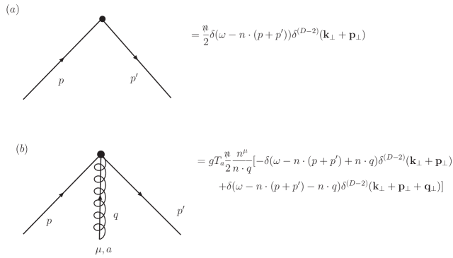
Figure 3: Feynman rules for the collinear operator $\mathcal{O}_{c}(\omega,{\bf k}_{\perp})$ to order $g$. In (b), $T_{a}$ are $SU(3)$ color generators, and the momentum of the collinear gluon is incoming.

Let us consider the radiative corrections for the collinear operator

$$\mathcal{O}_{c}(\omega,{\bf k}_{\perp})=\overline{\chi}_{\bar{n}}\frac{\hbox{$/$}\kern-5.50117pt\hbox{$n$}}{2}\delta(\omega-\mathcal{P}_{+})\delta^{(D-2)}({\bf k}_{\perp}+i{\bf\nabla}_{\perp})\chi_{n}.$$ (34)

The Feynman rules for the operator $\mathcal{O}_{c}$ to order $g$ is shown in Fig. 3 by expanding the collinear Wilson lines $W_{\bar{n}}$. The Feynman diagrams for the radiative correction at one loop is shown in Fig. 4. The computation is performed with dimensional regularization in $D=4-2\epsilon$ dimensions for the ultraviolet divergence and the nonzero external $p^{2}$ acts as an infrared cutoff. Note that the two-dimensional delta function in Eq. (34) becomes $(D-2)$-dimensional delta function in dimensional regularization. We can also use the two-dimensional delta function. While the above definition satisfies the rotational invariance in the $(D-2)$ transverse plane, the two-dimensional delta function breaks this symmetry. Though the symmetry is broken using the two-dimensional delta functions, the result for the radiative corrections can be made to be the same. Therefore the definition of the transverse delta function does not have to be unique, but it is preferable to keep the symmetry of the theory in dimensional regularization.

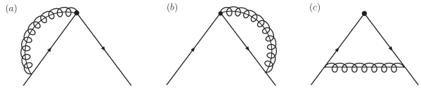
Figure 4: Feynman diagrams of the radiative correction for the collinear operator $\mathcal{O}_{c}$ at one loop.

Diagrams (a) and (b) in Fig. 4 yield

$$M_{a}=M_{b} = -2ig^{2}C_{F}\frac{\hbox{$/$}\kern-5.50117pt\hbox{$n$}}{2}\int\frac{d^{D}l}{(2\pi)^{D}}\frac{n\cdot(l+p)}{l^{2}(l+p)^{2}n\cdot l}\Bigl{[}\delta(\omega-\omega^{\prime})\delta^{(D-2)}({\bf k}_{\perp}+{\bf p}_{\perp})$$ (35)

$$-\delta(\omega-\omega^{\prime}-2n\cdot l)\delta^{(D-2)}({\bf l}_{\perp}+{\bf k}_{\perp}+{\bf p}_{\perp})\Bigr{]},$$

with $\omega^{\prime}=n\cdot p+n\cdot p^{\prime}$. The prescription for the poles is such that $+i0$ is added to each factor in the denominator. The first integral in Eq. (35) is simple because the delta functions do not involve the loop momentum, and it is given as

$$I_{1} = \int\frac{d^{D}l}{(2\pi)^{D}}\frac{n\cdot(l+p)}{l^{2}(l+p)^{2}n\cdot l}\delta(\omega-\omega^{\prime})\delta^{(D-2)}({\bf k}_{\perp})$$ (36)

$$= -\frac{i}{16\pi^{2}}\Bigl{(}\frac{-p^{2}}{\mu^{2}}\Bigr{)}^{-\epsilon_{\mathrm{UV}}}\frac{1}{\epsilon_{\mathrm{UV}}}\Bigl{(}-\frac{1}{\epsilon_{\mathrm{IR}}}-1\Bigr{)}\delta(\omega-\omega^{\prime})\delta^{(2-2\epsilon)}({\bf k}_{\perp}).$$

Note that there appear infrared poles of $\epsilon_{\mathrm{IR}}$ even though nonzero $p^{2}$ is introduced as the infrared cutoff. The second integral is more complicated and it is given by

$$I_{2}=-\int\frac{d^{D}l}{(2\pi)^{D}}\frac{n\cdot(l+p)}{l^{2}(l+p)^{2}n\cdot l}\delta(\omega-\omega^{\prime}-2n\cdot l)\delta^{(D-2)}({\bf l}_{\perp}+{\bf k}_{\perp}+{\bf p}_{\perp}).$$ (37)

After integrating the delta functions, the remaining integral can be performed using the contour integral in the complex $\overline{n}\cdot l$ plane. Depending on the position of the poles, the integral consists of two parts, each of which is proportional to $\theta(\omega^{\prime}-\omega)\theta(\omega)$ or $\theta(\omega-\omega^{\prime})\theta(-\omega)$. The first one corresponds to the contribution from a quark, while the second one is the antiquark contribution. Extracting only the contribution from a quark, the integral becomes

$$I_{2}=\frac{i}{16\pi^{3}}\frac{\omega}{\omega^{\prime}}\frac{\theta(\omega^{\prime}-\omega)\theta(\omega)}{\omega^{\prime}-\omega}\Bigl{[}\Bigl{(}{\bf k}_{\perp}+\frac{\omega}{\omega^{\prime}}{\bf p}_{\perp}\Bigr{)}^{2}+\frac{\omega(\omega^{\prime}-\omega)}{(\omega^{\prime})^{2}}\Bigl{(}\frac{-p^{2}}{\mu^{2}}\Bigr{)}\Bigr{]}^{-1}.$$ (38)

We can interpret the characteristics of the integrals $I_{1}$ and $I_{2}$ by tracing where each term arises. In $I_{1}$, the delta functions do not include the loop momentum. It means that $I_{1}$ comes from the combinations $\chi_{n}=W_{n}^{\dagger}\xi_{n}$ or $\overline{\chi}_{n}=\overline{\xi}W_{n}$ by extracting a collinear gluon and attaching it to the fermion on the same side with respect to the delta functions. On the other hand, $I_{2}$ comes from the configuration in which a gluon is attached to the fermion on the opposite side with respect to the delta functions. In other words, $I_{1}$ corresponds to the virtual correction and $I_{2}$ to the real gluon emission in the full theory. In inclusive deep inelastic scattering, the divergence of the form $1/(\epsilon_{\mathrm{UV}}\epsilon_{\mathrm{IR}})$ cancels between these two contributions Chay:2005rz . However, comparing Eqs. (36) and (38), the divergence does not seem to cancel. In the on-shell limit $p^{2}=0$, as $\omega^{\prime}\rightarrow\omega$ and ${\bf k}_{\perp}\rightarrow-{\bf p}_{\perp}$, $I_{2}$ diverges as

$$\frac{1}{\omega^{\prime}-\omega}\frac{1}{({\bf k}_{\perp}+{\bf p}_{\perp})^{2}},$$ (39)

but it does not cancel the divergence of the virtual gluon correction. Therefore it was claimed that if all the collinear particles were on the lightcone and the dimensional regularization was used, the divergence from the virtual and the real gluon corrections would not cancel unless an improved regularization technique was employed.

Here an improved renormalization technique is suggested using dimensional regularization, in which the divergences between the virtual and the real gluon corrections cancel. The point is that care must be taken in extracting a delta function in dimensional regularization. In Eq. (38), the interesting limit is $\omega^{\prime}\rightarrow\omega$ and ${\bf k}_{\perp}\rightarrow-{\bf p}_{\perp}$. The naive limit in Eq. (39) does not extract the correct singular behavior in dimensional regularization. Note that there is another parameter $-p^{2}$ in Eq. (38), which is introduced as an infrared cutoff. This can be made arbitrarily small before any physical limits are taken. Therefore the basic idea is that we have to take the limit $p^{2}\rightarrow 0$ first, and then take other limits. The dimensional regularization changes the short- and long-distance behavior of the loop integral, and the transverse momentum and the $n$-component of the momentum are closely related to each other as a result. By putting $p^{2}=0$ before any dependence on the dimension $D=4-2\epsilon$ is computed, it ruins this relation. In this respect, consider the limit

$$\lim_{a\rightarrow 0}\frac{1}{{\bf k}_{\perp}^{2}+a}.$$ (40)

As it is, it diverges when ${\bf k}_{\perp}\rightarrow 0$. However, we can consider the function

$$f(a,{\bf k}_{\perp})=\frac{a^{\delta}}{{\bf k}_{\perp}^{2}+a}$$ (41)

and take the limit $a\rightarrow 0$ such that $f(a,{\bf k}_{\perp})$ can be defined as a distribution function. As ${\bf k}_{\perp}\rightarrow 0$, $f(a,{\bf k}_{\perp})\sim a^{-1+\delta}$ and for ${\bf k}_{\perp}\neq 0$, $f(a,{\bf k}_{\perp})\sim a^{\delta}$. For $0<\delta<1$, $f(a,{\bf k}_{\perp})$ can be regarded as a representation of the delta function in the limit $a\rightarrow 0$, that is,

$$\lim_{a\rightarrow 0}\frac{a^{\delta}}{{\bf k}_{\perp}^{2}+a}=A\delta^{(D-2)}({\bf k}_{\perp}).$$ (42)

The normalization constant $A$ is independent of $a$, and is determined by the integral

$$\int\frac{d^{D-2}{\bf k}_{\perp}}{(2\pi)^{D-2}}\frac{a^{\delta}}{{\bf k}_{\perp}^{2}+a}=\frac{\Gamma(\epsilon)}{(4\pi)^{1-\epsilon}}a^{\delta-\epsilon}=\frac{A}{(2\pi)^{2-2\epsilon}}.$$ (43)

If we choose $\delta=\epsilon$, $A=\pi^{1-\epsilon}\Gamma(\epsilon)$. Therefore as $a\rightarrow 0$, we can write

$$\frac{1}{{\bf k}_{\perp}^{2}+a}\rightarrow\pi^{1-\epsilon}\Gamma(\epsilon)a^{-\epsilon}\delta^{(2-2\epsilon)}({\bf k}_{\perp}).$$ (44)

This holds for $0<\epsilon<1$, and it can be analytically continued for other values of $\epsilon$. The pole is of the ultraviolet origin, as can be seen from Eq. (43). When the representation of the delta function is used, it can be clearly seen that the momentum cutoff $|{\bf k}_{\perp}|<Q$ Lepage:1980fj cannot be used since the representation of a delta function is obtained only when all the range of the transverse momentum is included. Otherwise, there will be no cancellation of divergences, and the anomalous dimension will depend on the cutoff. Actually the integration should be performed for all ${\bf k}_{\perp}$ in SCET, since the upper bound for the effective theory is pulled up to infinity, and the modification of the high-energy behavior is implemented in the Wilson coefficients.

If Eq. (44) is applied to $I_{2}$, it becomes

$$I_{2} = \frac{i}{16\pi^{2}}\frac{\omega}{\omega^{\prime}}\Bigl{(}\frac{-p^{2}\omega}{\mu^{2}\omega^{\prime 2}}\Bigr{)}^{-\epsilon}(\omega^{\prime}-\omega)^{-1-\epsilon}\theta(\omega^{\prime}-\omega)\theta(\omega)\Gamma(\epsilon)\delta^{(2-2\epsilon)}\Bigl{(}{\bf k}_{\perp}+\frac{\omega}{\omega^{\prime}}{\bf p}_{\perp}\Bigr{)}$$

$$= \frac{i}{16\pi^{2}}\Bigl{(}\frac{-p^{2}}{\mu^{2}}\Bigr{)}^{-\epsilon}\Bigl{[}-\frac{1}{\epsilon_{\mathrm{UV}}\epsilon_{\mathrm{IR}}}\delta(\omega-\omega^{\prime})+\frac{1}{\epsilon_{\mathrm{UV}}}\frac{\omega}{\omega^{\prime}}\frac{\theta(\omega^{\prime}-\omega)}{(\omega^{\prime}-\omega)_{+}}\Bigr{]}\theta(\omega)\delta^{(2-2\epsilon)}\Bigl{(}{\bf k}_{\perp}+\frac{\omega}{\omega^{\prime}}{\bf p}_{\perp}\Bigr{)}.$$

We can write

$$(\omega^{\prime}-\omega)^{-1-\epsilon}\theta(\omega^{\prime}-\omega)\theta(\omega)=(\omega^{\prime})^{-1-\epsilon}(1-x)^{-1-\epsilon}\theta(1-x)\theta(x),$$ (46)

where $x=\omega/\omega^{\prime}$. When we integrate over $x$, the integral diverges at $x\approx 1$, which is of the infrared origin. Since the limits of the integral is bounded, there is no ultraviolet divergence and we obtain the formula

$$(\omega^{\prime}-\omega)^{-1-\epsilon}\theta(\omega^{\prime}-\omega)\theta(\omega)=\Bigl{[}-\frac{1}{\epsilon_{\mathrm{IR}}}\delta(\omega^{\prime}-\omega)+\frac{\theta(\omega^{\prime}-\omega)}{(\omega^{\prime}-\omega)_{+}}\Bigr{]}\theta(\omega),$$ (47)

with the $+$-distribution function. In the above expression, the divergence of the form $1/\epsilon_{\mathrm{UV}}\epsilon_{\mathrm{IR}}$ is cancelled in the sum $I_{1}+I_{2}$, and the amplitudes are given as

$$M_{a}=M_{b}=\frac{\alpha_{s}C_{F}}{4\pi}\frac{\hbox{$/$}\kern-5.50117pt\hbox{$n$}}{2}\frac{2}{\epsilon_{\mathrm{UV}}}\theta(\omega)\Bigl{[}\delta(\omega-\omega^{\prime})\delta^{(2-2\epsilon)}({\bf k}_{\perp})+\frac{\omega}{\omega^{\prime}}\frac{\theta(\omega^{\prime}-\omega)}{(\omega^{\prime}-\omega)_{+}}\delta^{(2-2\epsilon)}\Bigl{(}{\bf k}_{\perp}+\frac{\omega}{\omega^{\prime}}{\bf p}_{\perp}\Bigr{)}\Bigr{]}.$$ (48)

In a similar way, $M_{c}$ can be calculated to give

$$M_{c}=\frac{\alpha_{s}C_{F}}{4\pi}\frac{-2}{\epsilon_{\mathrm{UV}}}\delta^{(2-2\epsilon)}\Bigl{(}{\bf k}_{\perp}+\frac{\omega}{\omega^{\prime}}{\bf p}_{\perp}\Bigr{)}\frac{\omega^{\prime}-\omega}{\omega^{\prime 2}}\theta(\omega^{\prime}-\omega)\theta(\omega).$$ (49)

Adding all the contributions, we have

$$M_{a}+M_{b}+M_{c} = \frac{\alpha_{s}C_{F}}{2\pi}\frac{\hbox{$/$}\kern-5.50117pt\hbox{$n$}}{2}\frac{1}{\epsilon_{\mathrm{UV}}}\Bigl{[}2\delta(\omega-\omega^{\prime})\delta^{(2-2\epsilon)}({\bf k}_{\perp})$$ (50)

$$+ \frac{1+(\omega/\omega^{\prime})^{2}}{(\omega^{\prime}-\omega)_{+}}\theta(\omega^{\prime}-\omega)\theta(\omega)\delta^{(2-2\epsilon)}\Bigl{(}{\bf k}_{\perp}+\frac{\omega}{\omega^{\prime}}{\bf p}_{\perp}\Bigr{)}\Bigr{]}.$$

Now we have to subtract the zero-bin contribution Manohar:2006nz , which corresponds to the soft limit when the collinear loop momentum becomes soft, i.e., of order $\Lambda$. The collinear contribution from this soft region should be subtracted since collinear particles are defined to have large label momentum. This region should be described by soft particles, not by collinear particles with small label momenta. The loop integrals in $M_{a}+M_{b}+M_{c}$ were performed naively including the contribution of the collinear particles with small label momenta. Therefore this contribution should be subtracted. In computing the naive collinear contribution, the loop and the external momenta scale as

$$l^{\mu}=(n\cdot l,l_{\perp},\overline{n}\cdot l)\sim(Q,\Lambda,\Lambda^{2}/Q),\ \ p^{\mu}=(n\cdot p,p_{\perp},\overline{n}\cdot p)\sim(Q,\Lambda,\Lambda^{2}/Q),$$ (51)

But in computing the zero-bin contribution, we subtract the contribution where the largest component $n\cdot l$ becomes $\Lambda$, retaining the same scaling for $\overline{n}\cdot l$ and adjusting the scaling of $l_{\perp}$ such that $n\cdot l\overline{n}\cdot l\sim l_{\perp}^{2}$. Therefore the power counting of the loop and the external momenta is given by

$$l^{\mu}=(n\cdot l,l_{\perp},\overline{n}\cdot l)\sim(\Lambda,\Lambda\sqrt{\Lambda/Q},\Lambda^{2}/Q),\ \ p^{\mu}=(n\cdot p,p_{\perp},\overline{n}\cdot p)\sim(Q,\Lambda,\Lambda^{2}/Q).$$ (52)

One may wonder why the loop momentum of order $l^{2}\sim\Lambda^{3}/Q$ is subtracted, hence unphysical. That is exactly the reason why it should be subtracted from the collinear contribution and replaced by the soft contribution in which all the components of the momentum are of order $\Lambda$. We can also choose the power counting as $n\cdot l\sim\Lambda$, while others are fixed such that $l_{\perp}^{2}\gg n\cdot l\overline{n}\cdot l$, which is called the Glauber region. But it does not alter the result of the zero-bin contribution. The point of the zero-bin subtraction is to subtract the part in which energetic collinear particles become soft, and the criterion is the size of the label momentum.

According to the power counting in Eq. (52), the zero-bin contribution from the naive collinear integrals $M_{a}$ and $M_{b}$ are given as

$$M_{a}^{0}=M_{b}^{0} = -2ig^{2}C_{F}\frac{\hbox{$/$}\kern-5.50117pt\hbox{$n$}}{2}\int\frac{d^{D}l}{(2\pi)^{D}}\frac{1}{l^{2}(\overline{n}\cdot l+p^{2}/n\cdot p)n\cdot l}$$ (53)

$$\times\Bigl{[}\delta(\omega-\omega^{\prime})\delta^{(D-2)}({\bf k}_{\perp}+{\bf p}_{\perp})-\delta(\omega-\omega^{\prime}-2n\cdot l)\delta^{(D-2)}(\bf{k}_{\perp}+{\bf p}_{\perp})\Bigr{]},$$

and the zero-bin contribution from $M_{c}$ vanishes. The first integral is given by

$$J_{1} = \int\frac{d^{D}l}{(2\pi)^{D}}\frac{1}{l^{2}(\overline{n}\cdot l+p^{2}/n\cdot p)n\cdot l}\delta(\omega-\omega^{\prime})\delta^{(D-2)}({\bf k}_{\perp}+{\bf p}_{\perp})$$ (54)

$$= -\frac{i}{16\pi^{2}}\Bigl{(}\frac{-p^{2}}{\mu n\cdot p}\Bigr{)}^{-\epsilon_{\mathrm{UV}}}\Bigl{(}\frac{1}{\epsilon_{\mathrm{UV}}}-\frac{1}{\epsilon_{\mathrm{IR}}}\Bigr{)}\frac{1}{\epsilon_{\mathrm{UV}}}\delta(\omega-\omega^{\prime})\delta^{(2-2\epsilon)}({\bf k}_{\perp}+{\bf p}_{\perp}).$$

The second integral $J_{2}$ can be computed by integrating over the delta function first, doing the contour integral in the complex $\overline{n}\cdot l$ plane, and then finally integrating over $l_{\perp}$ using dimensional regularization. $J_{2}$ is given as

$$J_{2} = -\int\frac{d^{D}l}{(2\pi)^{D}}\frac{1}{l^{2}(\overline{n}\cdot l+p^{2}/n\cdot p)n\cdot l}\delta(\omega-\omega^{\prime}-2n\cdot l)\delta^{(D-2)}(\bf{k}_{\perp}+{\bf p}_{\perp})$$

$$= \frac{i}{16\pi^{2}}\frac{1}{\epsilon_{\mathrm{UV}}}\frac{\theta(\omega^{\prime}-\omega)}{\omega^{\prime}-\omega}\Bigl{(}\frac{(\omega^{\prime}-\omega)(-p^{2})}{n\cdot p\mu}\Bigr{)}^{-\epsilon_{\mathrm{UV}}}\delta^{(2-2\epsilon)}(\bf{k}_{\perp}+{\bf p}_{\perp})$$

$$= \frac{i}{16\pi^{2}}\Bigl{(}\frac{-p^{2}}{n\cdot p\mu}\Bigr{)}^{-\epsilon_{\mathrm{UV}}}\frac{1}{\epsilon_{\mathrm{UV}}}\Bigl{[}\Bigl{(}\frac{1}{\epsilon_{\mathrm{UV}}}-\frac{1}{\epsilon_{\mathrm{IR}}}\Bigr{)}\delta(\omega-\omega^{\prime})+\frac{\theta(\omega^{\prime}-\omega)}{(\omega^{\prime}-\omega)_{+}}\Bigr{]}\delta^{(2-2\epsilon)}(\bf{k}_{\perp}+{\bf p}_{\perp}),$$

where the following formula is used:

$$\theta(\omega^{\prime}-\omega)(\omega^{\prime}-\omega)^{-1-\epsilon}=\Bigl{(}\frac{1}{\epsilon_{\mathrm{UV}}}-\frac{1}{\epsilon_{\mathrm{IR}}}\Bigr{)}\delta(\omega^{\prime}-\omega)+\frac{\theta(\omega^{\prime}-\omega)}{(\omega^{\prime}-\omega)_{+}}.$$ (56)

The difference between this equation and Eq. (47) is that there is no lower bound. Therefore Eq. (56) has both infrared and ultraviolet singularity. In the sum $J_{1}+J_{2}$, the $\delta(\omega^{\prime}-\omega)$ term cancels and the zero-bin contribution is given by

$$M_{a}^{0}=M_{b}^{0}=\frac{\alpha_{s}C_{F}}{2\pi}\frac{\hbox{$/$}\kern-5.50117pt\hbox{$n$}}{2}\frac{2}{\epsilon_{\mathrm{UV}}}\frac{\theta(\omega^{\prime}-\omega)}{(\omega^{\prime}-\omega)_{+}}\delta^{(2-2\epsilon)}({\bf k}_{\perp}+{\bf p}_{\perp}).$$ (57)

Subtracting the zero-bin contribution, the total collinear contribution with the wavefunction renormalization is given by

$$M_{a}+M_{b}+M_{c}-(M_{a}^{0}+M_{b}^{0})+\mathrm{w.f.}$$ (58)

$$= \frac{\alpha_{s}C_{F}}{2\pi}\frac{\hbox{$/$}\kern-5.50117pt\hbox{$n$}}{2}\frac{2}{\epsilon_{\mathrm{UV}}}\Bigl{[}\Bigl{(}\frac{3}{2}\delta(\omega^{\prime}-\omega)-\frac{2}{(\omega^{\prime}-\omega)_{+}}\theta(\omega^{\prime}-\omega)\theta(\omega)\Bigr{)}\delta^{(2-2\epsilon)}({\bf k}_{\perp}+{\bf p}_{\perp})$$

$$+\frac{1+(\omega/\omega^{\prime})^{2}}{(\omega^{\prime}-\omega)_{+}}\theta(\omega^{\prime}-\omega)\theta(\omega)\delta^{(2-2\epsilon)}({\bf k}_{\perp}+\frac{\omega}{\omega^{\prime}}{\bf p}_{\perp})\Bigr{]},$$

where $\theta(\omega)$ in the second term is inserted for physical reasons. For comparison, the corresponding radiative correction for the collinear operator giving the integrated parton distribution function is given as Chay:2005rz

$$\frac{\alpha_{s}C_{F}}{2\pi}\frac{\hbox{$/$}\kern-5.50117pt\hbox{$n$}}{2}\frac{2}{\epsilon_{\mathrm{UV}}}\Bigl{[}\frac{3}{2}\delta(\omega^{\prime}-\omega)-\frac{2}{(\omega^{\prime}-\omega)_{+}}\theta(\omega^{\prime}-\omega)\theta(\omega)+\frac{1+(\omega/\omega^{\prime})^{2}}{(\omega^{\prime}-\omega)_{+}}\theta(\omega^{\prime}-\omega)\theta(\omega)\Bigr{]}.$$ (59)

This is the result from Eq. (58) without the delta functions of the transverse momentum, or by integrating over the transverse momentum. However, note that the radiative correction for the collinear TMD operator is not just proportional to $\delta^{(2-2\epsilon)}({\bf k}_{\perp}+{\bf p}_{\perp})$, but it also depends on $\delta^{(2-2\epsilon)}({\bf k}_{\perp}+(\omega^{\prime}/\omega){\bf p}_{\perp})$. This gives a nontrivial difference in the renormalization group behavior between the TMD and the integrated PDF.

IV.2 One loop correction to the soft Wilson line

We now compute the radiative corrections for the TMD soft Wilson line operator

$$S(\eta,{\bf s}_{\perp})=\frac{1}{N}\mathrm{tr}\,\tilde{Y}^{\dagger}_{\bar{n}}Y_{n}\delta(\eta+n\cdot i\partial)\delta^{(2)}({\bf s}_{\perp}+i\nabla_{\perp})Y_{n}^{\dagger}Y_{\bar{n}}.$$ (60)

The Feynman rule for the operator $S$ with two gluons is given in Fig. 5, and the Feynman diagram for the radiative correction at one loop is shown in Fig. 6. The radiative correction is written as

$$I(\eta,{\bf s}_{\perp}) = -2ig^{2}C_{F}\int\frac{d^{D}l}{(2\pi)^{D}}\Bigl{[}\frac{2\delta(\eta)\delta^{(D-2)}({\bf s}_{\perp})}{l^{2}(\overline{n}\cdot l-\lambda_{1})(n\cdot l-\lambda_{2})}$$

$$+ \frac{\delta(\eta+n\cdot l)\delta^{(D-2)}({\bf s}_{\perp}+{\bf l}_{\perp})}{(l^{2}+i0)(\overline{n}\cdot l-\lambda_{1}+i0)}\frac{1}{-n\cdot l+\lambda_{2}}+\frac{\delta(\eta-n\cdot l)\delta^{(D-2)}({\bf s}_{\perp}-{\bf l}_{\perp})}{(l^{2}+i0)(-\overline{n}\cdot l-\lambda_{1}+i0)}\frac{1}{n\cdot l+\lambda_{2}}\Bigr{]},$$

where $\lambda_{1}$ and $\lambda_{2}$ are the infrared cutoffs. And the necessary $i0$ prescriptions for the contour integral in the complex $\overline{n}\cdot l$ plane are shown.

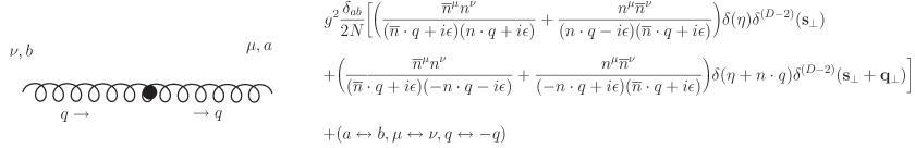
Figure 5: Feynman rules for the soft Wilson line operator $S(\eta,{\bf s}_{\perp})$ with two soft gluons.

Figure 6: Feynman diagram of one-loop correction for the TMD soft Wilson line.

The first integral is given by

$$S_{1} = -4ig^{2}C_{F}\int\frac{d^{D}l}{(2\pi)^{D}}\frac{\delta(\eta)\delta^{(D-2)}({\bf s}_{\perp})}{l^{2}(\overline{n}\cdot l-\lambda_{1})(n\cdot l-\lambda_{2})}$$ (62)

$$= -\frac{\alpha_{s}C_{F}}{2\pi}\frac{2}{\epsilon_{\mathrm{UV}}^{2}}\Bigl{(}\frac{\lambda_{1}\lambda_{2}}{\mu^{2}}\Bigr{)}^{-\epsilon}\delta(\eta)\delta^{(2-2\epsilon)}({\bf s}_{\perp}).$$

In the second and the third integrals in Eq. (IV.2), we perform the contour integration in the complex $\overline{n}\cdot l$ place after integrating over the delta functions. The second and the third integrals are given by

$$S_{2}=S_{3}=\frac{g^{2}C_{F}}{8\pi^{3}}\frac{\theta(\eta)}{\eta+\lambda_{2}}\frac{1}{{\bf s}_{\perp}^{2}+\eta\lambda_{1}}.$$ (63)

We apply the idea of the representation of the delta function again to have

$$\lim_{\lambda_{1}\rightarrow 0}\frac{1}{{\bf s}_{\perp}^{2}+\eta\lambda_{1}}=\frac{\pi^{1-\epsilon}}{\epsilon_{\mathrm{UV}}}(\eta\lambda_{1})^{-\epsilon}\delta^{(2-2\epsilon)}({\bf s}_{\perp}),$$ (64)

and the integral becomes

$$S_{2}=\frac{\alpha_{s}C_{F}}{2\pi}\frac{\theta(\eta)}{\epsilon_{\mathrm{UV}}}\frac{(\eta\lambda_{1})^{-\epsilon}}{\eta+\lambda_{2}}\delta^{(2-2\epsilon)}({\bf s}_{\perp})=\frac{\alpha_{s}C_{F}}{2\pi}\Bigl{[}\Bigl{(}\frac{\lambda_{1}\lambda_{2}}{\mu^{2}}\Bigr{)}^{-\epsilon}\frac{1}{\epsilon_{\mathrm{UV}}^{2}}+\frac{1}{\epsilon_{\mathrm{UV}}}\frac{\theta(\eta)}{\eta_{+}}\Bigr{]}\delta^{(2-2\epsilon)}({\bf s}_{\perp}).$$ (65)

Here the plus distribution function is also used. But note that all the poles in $1/\epsilon$ are of ultraviolet origin since the infrared cutoffs $\lambda_{1}$ and $\lambda_{2}$ are used. Adding all these, the radiative correction for the soft Wilson line at one loop is given by

$$I(\eta,{\bf s}_{\perp})=\frac{\alpha_{s}C_{F}}{\pi}\frac{1}{\epsilon_{\mathrm{UV}}}\frac{\theta(\eta)}{\eta_{+}}\delta^{(2-2\epsilon)}({\bf s}_{\perp}).$$ (66)

The only difference, compared with the integrated soft Wilson line Chay:2004zn , is the presence of $\delta^{(2-2\epsilon)}({\bf s}_{\perp})$. Therefore the anomalous dimension is the same as the integrated soft Wilson line except the delta function $\delta^{(2-2\epsilon)}({\bf s}_{\perp})$, that is, the TMD soft Wilson line does not scale with respect to the transverse momentum.

V Renormalization group behavior of the TMD operators

With the radiative corrections, the relations between the bare operators and the renormalized operators can be written, in general, as

$$\mathcal{O}_{c}^{B}(\omega,{\bf k}_{\perp};{\bf p}_{\perp}) = \int d\omega^{\prime}d^{D-2}{\bf k}^{\prime}_{\perp}Z_{C}(\omega,\omega^{\prime},{\bf k}_{\perp},{\bf k}^{\prime}_{\perp};{\bf p}_{\perp})\mathcal{O}_{c}^{R}(\omega^{\prime},{\bf k}_{\perp}^{\prime};{\bf p}_{\perp}),$$

$$S^{B}(\eta,{\bf s}_{\perp}) = \int d\eta^{\prime}d^{D-2}{\bf s}^{\prime}_{\perp}Z_{S}(\eta,\eta^{\prime},{\bf s}_{\perp},{\bf s}^{\prime}_{\perp})S^{R}(\eta^{\prime},{\bf s}^{\prime}_{\perp}),$$ (67)

where the counterterm kernels $Z_{C}(\omega,\omega^{\prime},{\bf k}_{\perp},{\bf k}^{\prime}_{\perp};{\bf p}_{\perp})$ and $Z_{S}(\eta,\eta^{\prime},{\bf s}_{\perp},{\bf s}^{\prime}_{\perp})$ can be read off from Eqs. (58) and (66), and are given as

$$Z_{C}(\omega,\omega^{\prime},{\bf k}_{\perp},{\bf k}^{\prime}_{\perp};{\bf p}_{\perp}) = \delta(\omega^{\prime}-\omega)\delta^{(2-2\epsilon)}({\bf k}_{\perp}-{\bf k}_{\perp}^{\prime})$$

$$+ \frac{\alpha_{s}C_{F}}{2\pi}\frac{\hbox{$/$}\kern-5.50117pt\hbox{$n$}}{2}\frac{2}{\epsilon_{\mathrm{UV}}}\Bigl{[}\Bigl{(}\frac{3}{2}\delta(\omega^{\prime}-\omega)-\frac{2\theta(\omega^{\prime}-\omega)\theta(\omega)}{(\omega^{\prime}-\omega)_{+}}\Bigr{)}\delta^{(2-2\epsilon)}({\bf k}_{\perp}-{\bf k}_{\perp}^{\prime})$$

$$+ \frac{1+(\omega/\omega^{\prime})^{2}}{(\omega^{\prime}-\omega)_{+}}\theta(\omega^{\prime}-\omega)\theta(\omega)\delta^{(2-2\epsilon)}({\bf k}_{\perp}-{\bf k}_{\perp}^{\prime}-\frac{\omega^{\prime}-\omega}{\omega^{\prime}}{\bf p}_{\perp})\Bigr{]},$$

$$Z_{S}(\eta,\eta^{\prime},{\bf s}_{\perp},{\bf s}^{\prime}_{\perp}) = \delta^{(2-2\epsilon)}({\bf s}_{\perp}-{\bf s}_{\perp}^{\prime})\Bigl{[}\delta(\eta-\eta^{\prime})+\frac{\alpha_{s}C_{F}}{\pi\epsilon_{\mathrm{UV}}}\frac{\theta(\eta-\eta^{\prime})}{(\eta-\eta^{\prime})_{+}}\Bigr{]}.$$ (68)

Here in $Z_{C}(\omega,\omega^{\prime},{\bf k}_{\perp},{\bf k}^{\prime}_{\perp};{\bf p}_{\perp})$, the external transverse momentum ${\bf p}_{\perp}$ of the quark is introduced for convenience, but it should be understood that it appears in the matrix element of the operator $\mathcal{O}_{c}$. The renormalization group equations for the renormalized operators are written as

$$\mu\frac{d}{d\mu}\mathcal{O}_{c}^{R}(\omega,{\bf k}_{\perp};{\bf p}_{\perp}) = -\int d\omega^{\prime}d^{2}{\bf k}_{\perp}^{\prime}\gamma_{C}(\omega,\omega^{\prime},{\bf k}_{\perp},{\bf k}^{\prime}_{\perp};{\bf p}_{\perp})\mathcal{O}_{c}^{R}(\omega^{\prime},{\bf k}_{\perp}^{\prime}),$$

$$\mu\frac{d}{d\mu}S^{R}(\eta,{\bf s}_{\perp}) = -\int d\eta^{\prime}d^{2}{\bf s}_{\perp}^{\prime}\gamma_{S}(\eta,\eta^{\prime},{\bf s}_{\perp},{\bf s}^{\prime}_{\perp})S^{R}(\eta^{\prime},{\bf s}_{\perp}^{\prime}),$$ (69)

where the anomalous dimension kernels are given by

$$\gamma_{C}(\omega,\omega^{\prime},{\bf k}_{\perp},{\bf k}^{\prime}_{\perp};{\bf p}_{\perp}) = -\frac{\alpha_{s}C_{F}}{\pi}\Bigl{[}\Bigl{(}\frac{3}{2}\delta(\omega-\omega^{\prime})-\frac{2\theta(\omega^{\prime}-\omega)\theta(\omega)}{(\omega^{\prime}-\omega)_{+}}\Bigr{)}\delta^{(2)}({\bf k}_{\perp}-{\bf k}_{\perp}^{\prime})$$

$$+ \frac{1+(\omega/\omega^{\prime})^{2}}{(\omega^{\prime}-\omega)_{+}}\theta(\omega^{\prime}-\omega)\theta(\omega)\delta^{(2)}({\bf k}_{\perp}-{\bf k}^{\prime}_{\perp}-\frac{\omega^{\prime}-\omega}{\omega^{\prime}}{\bf p}_{\perp})\Bigr{]},$$

$$\gamma_{S}(\eta,\eta^{\prime},{\bf s}_{\perp},{\bf s}^{\prime}_{\perp}) = -2\frac{\alpha_{s}C_{F}}{\pi}\delta^{(2)}({\bf s}_{\perp}-{\bf s}_{\perp}^{\prime})\frac{\theta(\eta-\eta^{\prime})}{(\eta-\eta^{\prime})_{+}}.$$ (70)

Note that the second term in $\gamma_{C}$ in Eq. (V), which corresponds to the zero-bin subtraction has the same form in $\gamma_{S}$ with the opposite sign. It confirms the nature of the zero-bin subtraction, which is computed in the soft limit. This pattern also appears in integrated PDF Chay:2005rz .

It is useful to express the renormalization group equation for $\mathcal{O}_{c}$ in terms of the dimensionless variables $y$ and $z$ defined as $\omega=2yn\cdot P_{\bar{n}}$, $\omega^{\prime}=2zn\cdot P_{\bar{n}}$, where $0<y,z<1$. It is given as

$$\mu\frac{d}{d\mu}\mathcal{O}_{c}(y,{\bf k}_{\perp};{\bf p}_{\perp})=-\int_{y}^{1}dz\int d^{2}{\bf k}_{\perp}^{\prime}\gamma_{C}(y,z,{\bf k}_{\perp},{\bf k}_{\perp}^{\prime};{\bf p}_{\perp})\mathcal{O}_{c}(z,{\bf k}_{\perp}^{\prime};{\bf p}_{\perp}),\$$ (71)

where

$$\gamma_{C}(y,z,{\bf k}_{\perp},{\bf k}_{\perp}^{\prime};{\bf p}_{\perp}) = -\frac{\alpha_{s}C_{F}}{\pi}\Bigl{[}\Bigl{(}\frac{3}{2}\delta(y-z)-\frac{2}{(z-y)_{+}}\Bigr{)}\delta^{(2)}({\bf k}_{\perp}-{\bf k}_{\perp}^{\prime})$$ (72)

$$+ \frac{1+(y/z)^{2}}{(z-y)_{+}}\delta^{(2)}\Bigl{(}{\bf k}_{\perp}-{\bf k}_{\perp}^{\prime}-\frac{z-y}{z}{\bf p}_{\perp}\Bigr{)}\Bigr{]}.$$

In terms of $x=y/z$, Eq. (71) becomes

$$\mu\frac{d}{d\mu}\mathcal{O}_{c}(y,{\bf k}_{\perp};{\bf p}_{\perp}) = \frac{\alpha_{s}C_{F}}{\pi}\int d^{2}{\bf k}^{\prime}_{\perp}\int_{y}^{1}\frac{dx}{x}\Bigl{[}\Bigl{(}\frac{3}{2}\delta(1-x)-\frac{2}{(1-x)_{+}}\Bigr{)}\delta^{(2)}({\bf k}_{\perp}-{\bf k}_{\perp}^{\prime})$$ (73)

$$+ \frac{1+x^{2}}{(1-x)_{+}}\delta^{(2)}({\bf k}_{\perp}-{\bf k}_{\perp}^{\prime}-(1-x){\bf p}_{\perp})\Bigr{]}\mathcal{O}_{c}(y/x,{\bf k}_{\perp}^{\prime};{\bf p}_{\perp}).$$

Note that, from Eq. (27), the matrix element of the collinear operator $\mathcal{O}_{c}$ is given by

$$g(y,-{\bf k}_{\perp})=\langle P_{\bar{n}}|\mathcal{O}_{c}(\omega=2yn\cdot P_{\bar{n}},{\bf k}_{\perp})|P_{\bar{n}}\rangle.$$ (74)

Then Eq. (71) can be expressed in impact parameter representation, or its Fourier transform as

$$\mu\frac{d}{d\mu}\tilde{g}(y,{\bf b}_{\perp}) = \mu\frac{d}{d\mu}\int d^{2}{\bf k}_{\perp}e^{i{\bf b}_{\perp}\cdot{\bf k}_{\perp}}g(y,-{\bf k}_{\perp})$$

$$= \frac{\alpha_{s}C_{F}}{\pi}\int_{y}^{1}dz\Bigl{[}\frac{3}{2}\delta(y-z)+\frac{-2+(1+(y/z)^{2})e^{i(1-y/z){\bf b}_{\perp}\cdot{\bf p}_{\perp}}}{(z-y)_{+}}\Bigr{]}\tilde{g}(z,{\bf b}_{\perp}),$$

where the sign of the exponent becomes opposite compared to Eq. (III) since the 4-vector notation is changed to the 3-vector notation here. If we put ${\bf b}_{\perp}=0$ in Eq. (V), both sides become the integrated quantities over the transverse momentum ${\bf k}_{\perp}$, and the corresponding renormalization group equation is given by

$$\mu\frac{d}{d\mu}\int d^{2}{\bf k}_{\perp}g(y,{\bf k}_{\perp})=\frac{\alpha_{s}}{\pi}\int_{y}^{1}\frac{dx}{x}\Bigl{(}P_{qq}(x)-\frac{2C_{F}}{(1-x)_{+}}\Bigr{)}\int d^{2}{\bf k}_{\perp}g(y/x,{\bf k}_{\perp}),$$ (76)

where $P_{qq}(x)$ is the quark splitting function given by

$$P_{qq}(x)=C_{F}\Bigl{[}\frac{3}{2}\delta(1-x)+\frac{1+x^{2}}{(1-x)_{+}}\Bigr{]}.$$ (77)

An extra term in Eq. (76) other than $P_{qq}(x)$ comes from the zero-bin subtraction. Eq. (76) is exactly the same renormalization group equation for the integrated collinear operator in Ref. Chay:2005rz .

The renormalization group equation for the TMD soft Wilson line after integrating over ${\bf s}_{\perp}^{\prime}$ in Eq. (V) is written as

$$\mu\frac{d}{d\mu}S(\eta,{\bf s}_{\perp})=\frac{2\alpha_{s}C_{F}}{\pi}\int d\eta^{\prime}\frac{\theta(\eta-\eta^{\prime})}{(\eta-\eta^{\prime})_{+}}S(\eta^{\prime},{\bf s}_{\perp}).$$ (78)

Since the anomalous dimension for the TMD soft Wilson line is proportional to $\delta({\bf s}_{\perp}-{\bf s}_{\perp}^{\prime})$, the transverse-momentum-dependent part is trivial and the TMD soft Wilson line does not scale with respect to the transverse momentum. As a result, the renormalization group equation for the TMD soft Wilson line is the same as the integrated soft Wilson line Chay:2004zn .

Besides the renormalization group equation, the radiative corrections themselves, when integrated over the transverse momentum, give the same result for the radiative correction of the integrated collinear operator. If the counterterm kernels in Eq. (V) is integrated over the transverse momentum, the results correspond to the counterterm kernels for the integrated collinear and soft Wilson line operators. Therefore the relation between the TMD (unintegrated) and integrated PDF can be clearly seen in this formulation. That is, the integrated PDF and its renormalization group behavior are obtained by integrating the TMD PDF and its renormalization group equation over the transverse momentum. We can see this relation explicitly. From Eq. (26), the renormalization group equation for $f(y,{\bf p}_{\perp},\kappa)$ is written as

$$\mu\frac{d}{d\mu}f(y,{\bf p}_{\perp},\kappa) = \int d^{2}{\bf s}_{\perp}d^{2}{\bf k}_{\perp}\delta^{(2)}({\bf p}_{\perp}+{\bf k}_{\perp}+{\bf s}_{\perp})$$ (79)

$$\times \Bigl{[}\Bigl{(}\mu\frac{d}{d\mu}g(y,-{\bf k}_{\perp})\Bigr{)}K(\kappa,{\bf s}_{\perp})+g(y,-{\bf k}_{\perp})\Bigl{(}\mu\frac{d}{d\mu}K(\kappa,{\bf s}_{\perp})\Bigr{)}\Bigr{]}$$

$$= -\int d^{2}{\bf s}_{\perp}d^{2}{\bf k}_{\perp}\delta^{(2)}({\bf p}_{\perp}+{\bf k}_{\perp}+{\bf s}_{\perp})\int d^{2}{\bf s}_{\perp}^{\prime}d^{2}{\bf k}_{\perp}^{\prime}dzd\kappa^{\prime}$$

$$\times \gamma_{f}(y,z,{\bf k}_{\perp},{\bf k}_{\perp}^{\prime};\kappa,\kappa^{\prime},{\bf s}_{\perp},{\bf s}_{\perp}^{\prime};{\bf p}_{\perp})g(z,-{\bf k}_{\perp}^{\prime})K(\kappa^{\prime},{\bf s}_{\perp}^{\prime}),$$

where

$$\gamma_{f}(y,z,{\bf k}_{\perp},{\bf k}_{\perp}^{\prime};\kappa,\kappa^{\prime},{\bf s}_{\perp},{\bf s}_{\perp}^{\prime};{\bf p}_{\perp}) = \gamma_{C}(y,z,{\bf k}_{\perp},{\bf k}_{\perp}^{\prime};{\bf p}_{\perp})\delta(\kappa-\kappa^{\prime})\delta^{(2)}({\bf s}_{\perp}-{\bf s}_{\perp}^{\prime})$$ (80)

$$+ \gamma_{S}(\kappa,\kappa^{\prime},{\bf s}_{\perp},{\bf s}_{\perp}^{\prime})\delta(y-z)\delta^{(2)}({\bf k}_{\perp}-{\bf k}_{\perp}^{\prime}).$$

This is a complicated integro-differential equation. But it is more convenient to derive the renormalization group equation in impact parameter space. From Eq. (30), the renormalization group equation for $\tilde{f}(y,{\bf b}_{\perp},\kappa)$ is given by

$$\mu\frac{d}{d\mu}\tilde{f}(y,{\bf b}_{\perp},\kappa) = \Bigl{(}\mu\frac{d}{d\mu}\tilde{g}(y,{\bf b}_{\perp})\Bigr{)}\tilde{K}(\kappa,-{\bf b}_{\perp})+\tilde{g}(y,{\bf b}_{\perp})\Bigl{(}\mu\frac{d}{d\mu}\tilde{K}(\kappa,-{\bf b}_{\perp})\Bigr{)}.$$ (81)

Each $\tilde{g}(y,{\bf b}_{\perp})$ and $\tilde{K}(\kappa,-{\bf b}_{\perp})$ satisfies the renormalization group equation

$$\mu\frac{d}{d\mu}\tilde{g}(y,{\bf b}_{\perp}) = \mu\frac{d}{d\mu}\int d^{2}{\bf k}_{\perp}e^{i{\bf b}_{\perp}\cdot{\bf k}_{\perp}}g(y,-{\bf k}_{\perp})$$

$$= \frac{\alpha_{s}C_{F}}{\pi}\int_{y}^{1}dz\Bigl{[}\frac{3}{2}\delta(y-z)+\frac{-2+(1+(y/z)^{2})e^{i(1-y/z){\bf b}_{\perp}\cdot{\bf p}_{\perp}}}{(z-y)_{+}}\Bigr{]}\tilde{g}(z,{\bf b}_{\perp}),$$

$$\mu\frac{d}{d\mu}\tilde{K}(\kappa,-{\bf b}_{\perp}) = \frac{2\alpha_{s}C_{F}}{\pi}\int d\kappa^{\prime}\frac{\theta(\kappa-\kappa^{\prime})}{(\kappa-\kappa^{\prime})_{+}}\tilde{K}(\kappa^{\prime},-{\bf b}_{\perp}).$$ (83)

Therefore Eq. (81) is written as

$$\mu\frac{d}{d\mu}\tilde{f}(y,{\bf b}_{\perp},\kappa)=-\int dzd\kappa^{\prime}\tilde{\gamma}_{f}(y,z,\kappa,\kappa^{\prime};{\bf b}_{\perp},{\bf p}_{\perp})\tilde{f}(z,{\bf b}_{\perp},\kappa^{\prime}),$$ (84)

where

$$\tilde{\gamma}_{f}(y,z,\kappa,\kappa^{\prime};{\bf b}_{\perp},{\bf p}_{\perp}) = -\frac{\alpha_{s}C_{F}}{\pi}\Bigl{[}\Bigl{(}\frac{3}{2}\delta(y-z)+\frac{-2+(1+(y/z)^{2})e^{i(1-y/z){\bf b}_{\perp}\cdot{\bf p}_{\perp}}}{(z-y)_{+}}\Bigr{)}\delta(\kappa-\kappa^{\prime})$$ (85)

$$+ \frac{2\theta(\kappa-\kappa^{\prime})}{(\kappa-\kappa^{\prime})_{+}}\delta(y-z)\Bigr{]}.$$

This is the main result for the renormalization group behavior of the TMD collinear operator. For ${\bf b}_{\perp}=0$ in Eq. (85), we obtain the renormalization group equation for the integrated PDF.

VI Conclusion

It is shown that the hadronic tensor, hence the scattering cross section in SIDIS is factorized into a hard part, the TMD PDF, and the fragmentation function. The TMD PDF is further factorized into the TMD collinear part and the TMD soft Wilson lines. The TMD PDF is defined in terms of the matrix element of the gauge invariant TMD collinear operator in which all the collinear particles are put on the lightcone with no extra Wilson lines off the lightcone. The TMD soft Wilson is defined in a similar way. The radiative correction for the TMD PDF is computed with the zero-bin subtraction, and is shown that the divergences of the form $1/(\epsilon_{\mathrm{UV}}\epsilon_{\mathrm{IR}})$ are cancelled. This cancellation is obtained by using the representation of a delta function before the parameter $\epsilon$ in dimensional regularization is set to zero. The resultant anomalous dimension kernel shows a nontrivial dependence on the momentum fraction $x$ and the transverse momentum ${\bf p}_{\perp}$ of the incoming parton. The radiative correction for the TMD soft Wilson line is also performed and the anomalous dimension kernel is the same as the integrated soft Wilson line except the delta function for the transverse momentum. That is, the TMD soft Wilson line does not scale with respect to the transverse momentum and it shows the same scaling behavior as that of the integrated soft Wilson line.

There are several issues in obtaining the TMD PDF and its renormalization group behavior. In contrast to previous approaches, all the collinear particles, hence all the collinear and soft Wilson lines are on the lightcone. The cancellation of the divergence with the form $1/(\epsilon_{\mathrm{UV}}\epsilon_{\mathrm{IR}})$ in the radiative correction of the TMD quantities is explicitly shown by carefully taking care of the limiting behavior of the calculation in dimensional regularization. Since the transverse momentum and the $n$-component of the collinear momentum are closely related to each other in dimensional regularization, if we put the parameter $\epsilon$ in dimensional regularization to zero in the first place, the calculation becomes inconsistent and the cancellation does not occur, as claimed before. The technique used here is to introduce external $p^{2}$ as an infrared cutoff and treat the ultraviolet divergence in dimensional regularization. Though there is an infrared cutoff, not all the infrared divergences are expressed in terms of the cutoff, but there are some divergences which appear as poles of $\epsilon_{\mathrm{IR}}$. It is important to disentangle all the types of these divergences along with the ultraviolet divergence. After adding all the contributions, the infrared poles of $\epsilon_{\mathrm{IR}}$ are cancelled. Especially, the problematic divergence is of the form $1/(\epsilon_{\mathrm{UV}}\epsilon_{\mathrm{IR}})$ which should not be present in order for the theory to make sense. In this approach there is no need to introduce additional soft Wilson lines which offers a counterterm to cancel the divergence from the virtual correction. Instead the use of the representation of a delta function and the plus function prescription are employed to show the cancellation of the unwanted divergence.

In evaluating the radiative corrections, the external nonzero $p^{2}$ is introduced as an infrared cutoff and the limit $p^{2}\rightarrow 0$ is taken first before considering other limits. It is claimed that putting $p^{2}=0$ before the calculation in dimensional regularization would yield an incorrect result. Then a question can be raised about whether the extraction of divergence is possible with the on-shell scheme ($p^{2}=0$) and treat both the infrared and the ultraviolet divergences using dimensional regularization. This is in principle possible, but it is extremely challenging to trace the origin of the divergences. In this case, however, the calculation with nonzero $p^{2}$ can be a guideline to trace the divergences.

The zero-bin subtraction is also important in avoiding double counting. In computing the radiative corrections of the collinear operator, the integrals were computed naively including the unphysical region with small label momentum. This region should be subtracted because that region is covered by soft particles. Otherwise, double counting occurs. The true soft contribution is decoupled from the collinear part, and it appears in the soft Wilson line.

The renormalization group equation for the TMD collinear operator is a complicated integro-differential equation in which the momentum fraction $x$ appears in the delta function for the transverse momentum. In impact parameter space, the renormalization group equation involves an oscillating term which makes it difficult to solve the equation. However the renormalization group equations involve only physical variables. In contrast to previous approaches, this equation does not involve the rapidity parameter $\zeta$ Collins:1981uk , or the mass parameters $m$ and $\lambda$ Ji:2004wu , therefore it is difficult to compare the renormalization group equation or the radiative corrections directly.

The comparison between the TMD (or unintegrated) PDF or soft Wilson lines and the integrated PDF or soft Wilson lines becomes manifest in this approach. In this paper, it is shown by explicit calculation at one loop that the radiative corrections and the renormalization group equations for the integrated PDF and soft Wilson line are obtained by integrating those for the unintegrated (or TMD) PDF and soft Wilson lines over the transverse momentum. This is different from previous approach in which the comparison was not transparent because the order of integrating over the transverse momentum and the removal of the divergence makes the comparison difficult Ji:2004wu . However the calculational procedure in this paper makes the comparison clear.

Here the TMD PDF is considered only for quark distribution functions. But it is straightforward to extend the idea, and calculate the radiative corrections for gluon distribution functions and their mixing at higher orders in $\alpha_{s}$. The analysis on the TMD collinear, soft operators and their renormalization group behavior can be extended to other high-energy processes such as jet production or Drell-Yan processes (for full QCD approach, see Refs. Collins:1981uk and Collins:1982wa ). There will appear appropriate collinear and soft operators, but the form and structure of these operators might be different. It would be interesting to consider other high-energy processes and to see if there are important processes in which the transverse-momentum-dependent effects are relevant.

References

- (1) J. C. Collins and D. E. Soper, Nucl. Phys. B 193, 381 (1981) [Erratum-ibid. B 213, 545 (1983)].
- (2) J. C. Collins and D. E. Soper, Nucl. Phys. B 194, 445 (1982).
- (3) J. C. Collins, Acta Phys. Polon. B 34, 3103 (2003).
- (4) X. d. Ji, J. p. Ma and F. Yuan, Phys. Rev. D 71, 034005 (2005).
- (5) J. C. Collins and F. Hautmann, Phys. Lett. B 472, 129 (2000); F. Hautmann, Phys. Lett. B 655, 26 (2007).
- (6) I. O. Cherednikov and N. G. Stefanis, arXiv:0710.1955 [hep-ph].
- (7) C. W. Bauer, S. Fleming and M. E. Luke, Phys. Rev. D 63, 014006 (2001).
- (8) C. W. Bauer, S. Fleming, D. Pirjol and I. W. Stewart, Phys. Rev. D 63, 114020 (2001).
- (9) C. W. Bauer, D. Pirjol and I. W. Stewart, Phys. Rev. D 65, 054022 (2002).
- (10) C. W. Bauer, S. Fleming, D. Pirjol, I. Z. Rothstein and I. W. Stewart, Phys. Rev. D 66, 014017 (2002).
- (11) A. V. Manohar, Phys. Rev. D 68, 114019 (2003).
- (12) J. Chay and C. Kim, Phys. Rev. D 75, 016003 (2007).
- (13) T. Becher, M. Neubert and B. D. Pecjak, JHEP 0701, 076 (2007).
- (14) P. y. Chen, A. Idilbi and X. d. Ji, Nucl. Phys. B 763, 183 (2007).
- (15) A. Idilbi and T. Mehen, Phys. Rev. D 75, 114017 (2007).
- (16) J. Chay, C. Kim, Y. G. Kim and J. P. Lee, Phys. Rev. D 71, 056001 (2005).
- (17) G. P. Korchemsky and G. Marchesini, Nucl. Phys. B 406, 225 (1993).
- (18) G. P. Lepage and S. J. Brodsky, Phys. Rev. D 22, 2157 (1980).
- (19) A. V. Manohar and I. W. Stewart, Phys. Rev. D 76, 074002 (2007).
- (20) J. C. Collins, D. E. Soper and G. Sterman, Nucl. Phys. B 223, 381 (1983).